Spontaneous Collapse of Unstable Quantum Superposition State

Abstract

On the basis of a proposed model of wave function collapse, we investigate spontaneous localization of a quantum state. The model is similar to the Ghirardi-Rimini-Weber model, while we postulate the localization functions to depend on the quantum state to suffer collapse. According to the model, dual dynamics in quantum mechanics, deterministic and stochastic time evolution, are algorithmically implemented in tandem. After discussing the physical implications of the model qualitatively, we present numerical results for one-dimensional systems by way of example.

I Introduction

There has been a significant increase of interest in the foundations of quantum mechanics (QM). This owes undoubtedly to the technological progress achieved during the last decades in experimental investigation of how quantum systems behave not only statistically, but on an individual level. In fact, there are experimental results for microscopic systems which appear to be naturally explained by resorting to collapse of wave functionCohen-Tannoudji and Dalibard (1986); Poratti and Putterman (1987); Sauter et al. (1986); Cook (1988); Blatt and Zoller (1988); Pegg and Knight (1988); Ambrose and Moerner (1991); Ralls and Buhrman (1988); Bergquist et al. (1986); Nagourney et al. (1986); Leibfried et al. (2003). Notwithstanding, wave function collapse has ever been the source of the problem in understanding and interpreting QM, and there is still no definitive consensus on the “measurement” problem. Accordingly, along with those which accept the collapse postulate, there are many other interpretations, such as de Broglie-Bohm causal interpretationBohm (1952a); Holland (1993); Dürr et al. (1992), statistical interpretationBallentine (1970), decoherenceZeh (1970); Machida and Namiki (1980a); Joos and Zeh (1985); Namiki and Pascazio (1993); Giulini et al. (1996); Zurek (2003), modal interpretationsvan Frassen (1991); Healey (1989); Vermaas and Dieks (1998), consistent (decoherent) historiesGriffiths (1984); Omnès (1992); Gell-Mann and Hartle (1990), many-worlds/minds interpretationsEverett III (1957); DeWitt and Graham (1973); Deutsch (1985); Albert and Loewer (1988); Albert (1992). In this paper, we aim to investigate a realistic model of wave function collapse.

First of all, it is totally unsatisfactory to connect wave function collapse with an act of measurement, because the concept of measurement is ill-definedBell (1981, 1990). To describe wave function collapse from a realistic standpoint, we have to specify a well-defined dynamics of the stochastic process of collapse. In this regard, there are long-standing studies on stochastic nonlinear equations to realize collapse effectively. On the one hand, models to cause rapid but continuous collapse in the sense of Brownian motion were studied by Bohm and BubBohm and Bub (1966), PearlePearle (1976), DiósiDiósi (1985), and GisinGisin (1984a). On the other hand, a model postulating discontinuous instantaneous collapse was elaborated in the pioneering work by Ghirardi, Rimini and Weber (GRW)Ghirardi et al. (1986); Bell (1987a). At present, the GRW model and the Pearle model have been jointly developed to the continuous spontaneous localization (CSL) modelGhirardi et al. (1990). Mathematically, CSL is based on a stochastically modified Schrödinger equation. The current status of studies on what are and have to be achieved in their models has been reviewed extensivelyGhirardi (2000); Bassi and Ghirardi (2003); Pearle (1999); Pearle et al. (1999). On the basis of the idea of spontaneous collapse (SC), which may have a clue to the measurement problem, a good deal of related works are published indeedFrenkel (1990); Milburn (1991); Percival (1995); Hughston (1996); Adler and Howritz (2000). The task of theories based on and accounting for SC is to specify when, how and how often the collapse occurs, and to investigate the physical consequences. This is particularly important because the effect of SC must be physically relevant, in striking contrast to the other interpretations. The predictions of collapse theories should more or less deviate from those of standard quantum mechanics (SQM).

In this paper, we propose and investigate another such model of similar physical implications as the original GRW model. We also introduce two constants to characterize the dynamics of collapse. In the GRW model, a wave function is subjected to incessant spontaneous localizations, or the wave function is multiplied by a localization function, e.g., the Gaussian function, of which the frequency and the localization width are postulated to be universal constants, $\lambda\simeq 10^{-16}$sec^-1 and $a\simeq 10^{-5}$cm, respectively. The GRW localization mechanism is such that its frequency increases as the number $N$ of constituents of a composite system increases, so that a macroscopic object comprising an Avogadro number of constituents collapses extremely rapidly, at a rate of $N\lambda\simeq 10^{7}$sec^-1. In contrast, we propose to postulate a constant collapse rate $\gamma_{0}=\tau_{0}^{-1}$, while we model that the localization functions, particularly its length scale, are variable and depend on the wave function to suffer collapse. In effect, we introduce an energy scale $T_{0}$ so that the stochastic collapse should occur to the effect to cost energy $\Delta E\simeq T_{0}$. Therefore, in our model, the macroscopic number $N$ does not play any essential role, so that the effect of collapse may manifest itself even in microscopic systemstoa .

After introducing our collapse model in Section II.1, we discuss the physical implications of the model in Section II.2 and in Section III. By way of illustration, in Section IV, we apply the modified dynamics to obtain numerical results for one-dimensional systems. Although we are mainly interested in the individual dynamical evolution of a particular system, we briefly discuss the statistical description of the system in terms of the density matrix in Section V. We state our conclusion in Section VI. In Appendix A, we give an analytical treatment of a simple special case of the model to support general discussions in the main text. We discuss a generalization required to treat many particle systems in Appendix B. The main purpose of this paper is to show that the proposed model provides us with a consistent picture of crossover between quantum and classical mechanics.

II Model

II.1 Single particle problem

We discuss a non-relativistic model of spontaneous collapse. Let us consider the normalized state $\Psi_{t}({\bf r})$ as a function of space ${\bf r}$ and time $t$, where the indices representing internal quantum degrees of freedom like spins are suppressed for simplicity. We postulate that $\Psi_{t+\Delta t}({\bf r})$ after the infinitesimal elapse of time $\Delta t$ is determined from $\Psi_{t}({\bf r})$ stochastically as follows: (i) With the probability $\gamma_{0}\Delta t$,

$$\Psi_{t+\Delta t}({\bf r})=\left(1-\frac{{\rm i}}{\hbar}\hat{H}\Delta t\right)\Psi_{t}({\bf r}),$$ (1)

while (ii)

$$\Psi_{t+\Delta t}({\bf r})=\Phi_{n}({\bf r})\equiv\frac{1}{\sqrt{w_{n}}}P_{n}({\bf r})\Psi_{t}({\bf r}),$$ (2)

with the probability $(1-\gamma_{0})w_{n}\Delta t$, where

$$w_{n}\equiv\int{\rm d}{\bf r}|\Psi_{t}({\bf r})|^{2}P_{n}({\bf r})^{2}.$$ (3)

In (3), the sum over the suppressed indices is implicit in the definition of the modulus square $\rho({\bf r})=|\Psi_{t}({\bf r})|^{2}$, which thus represents the density in ordinary space. Unlike (i), the process (ii) is discontinuous by postulate, so that it cannot be put into a differential equation, though we can take the limit $\Delta t\rightarrow 0$ without affecting the physical content of the model. The branching structure of the proposed dynamics is schematically summarized in Fig. 1. According to the modified dynamics, the quantum state $\Psi({\bf r})$ is subjected to collapse (ii) with the constant rate $\gamma_{0}$. The probability to keep following the deterministic evolution (i) for $N\Delta t=\tau$ is given by $\left(1-\frac{\gamma_{0}\tau}{N}\right)^{N}\rightarrow\exp\left(-\gamma_{0}\tau\right)$ as $N\rightarrow\infty$. The collapse rate $\gamma_{0}$, or the time $\tau_{0}=\gamma_{0}^{-1}$, is the first parameter of our model.

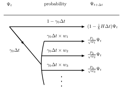
Figure 1: Flow chart of the modified dynamics. From the initial state in the left, one (and only one) of the states in the right column is realized with the probability attached to the arrow.

In (2), the effect of collapse is described by the real-valued continuous envelop functions $P_{n}({\bf r})$, which we call the localization functions, following the GRW model. The factor $\sqrt{w_{n}}$ in (2) is to normalize the collapse outcomes, $\langle\Phi_{n}|\Phi_{n}\rangle=1$. The functions $P_{n}({\bf r})$ have to satisfy

$$\sum_{n}P_{n}({\bf r})^{2}=1,\qquad 0\leq P_{n}({\bf r})\leq 1,$$ (4)

in order to meet the conservation of probability,

$$\sum_{n}w_{n}=1.$$ (5)

To achieve spontaneous localization, the GRW model assumes $P_{n}({\bf r})$ to be the Gaussian functions with a fixed width centered at random positions. We postulate rather that a set of the real functions $P_{n}({\bf r})$ is determined optimally depending on the state $\Psi_{t}({\bf r})$ so as to maximize

$$S^{\prime}=\sum_{n}w_{n}\int|\Phi_{n}|^{2}\log|\Phi_{n}|^{2}{\rm d}{\bf r},$$ (6)

under the constraint

$$T_{0}\Delta S=\Delta E,$$ (7)

where

$$\Delta S = -{\rm Tr}(\hat{\rho}\log\hat{\rho})$$ (8)

and

$$\Delta E = {\rm Tr}(\hat{\rho}\hat{H})-\langle\Psi|\hat{H}|\Psi\rangle.$$ (9)

are the physical changes of entropy and energy due to collapse. They are defined customarily in terms of the density matrix $\hat{\rho}=\hat{\rho}_{t+\Delta t}$ of the collapse outcome. In real space representation, the matrix elements of $\hat{\rho}$ are given by

$$\langle{\bf r}|\hat{\rho}|{\bf r^{\prime}}\rangle = \sum_{n}w_{n}\Phi_{n}({\bf r})^{*}\Phi_{n}({\bf r}^{\prime}).$$ (10)

The above is the procedure that we propose to fix the collapse outcomes $\tilde{\Phi}_{n}=P_{n}{\Psi}$ resulting from an arbitrary state $\Psi$. From our standpoint to regard wave function collapse as a real process, (8) and (9) represent the physical changes accompanied by the collapse, both of which are the important quantities to characterize the stochastic irreversible process. Thus (7) and (4) respectively represent statistical conservation of ‘free energy’ $F=E-T_{0}S$ and the density,

$$|\Psi({\bf r})|^{2}=\sum_{n}|\tilde{\Phi}_{n}({\bf r})|^{2}.$$ (11)

Under these statistical constraints, we obtain the set of collapse outcomes $\tilde{\Phi}_{n}$ by modifying to replace the squared amplitude $\rho$ of the initial state $\Psi=\sqrt{\rho}{\rm e}^{{\rm i}\alpha}$ with $\tilde{\rho}_{n}\equiv P_{n}^{2}\rho$ without affecting the phase $\alpha$. Thus, in a sense, we envisage the collapse as a kind of fragmentation of wave packet $\rho\rightarrow\{\tilde{\rho}_{n}\}$ in real space.

In case where there happens to be non-equivalent sets of the localization functions $\{P_{n}\}$ for given $\Psi_{t}({\bf r})$, e.g., by reason of symmetry, we require another postulate that a single set is chosen from among them at random with equal a priori probability. It would be clear that these postulates to formulate the probabilistic ‘second law’ (2) are adopted on the analogy drawn from Thermodynamics of the irreversible process of open systems immersed in a heat bath at temperature $T_{0}$. The constant $T_{0}$ is the second parameter of our model.

We adopt (6) as a proper expression to implement the spontaneous tendency of collapse to reduce the spatial extent of the quantum state,

$$(\delta{\bf r})^{2} = \sum_{n}w_{n}\left({\langle\Phi_{n}|{\bf r}\cdot{\bf r}|\Phi_{n}\rangle}-|{\langle\Phi_{n}|{\bf r}|\Phi_{n}\rangle}|^{2}\right).$$ (12)

Thus we take account of the special role of the position basis in terms of $S^{\prime}$. In effect, to minimize the variance $(\delta{\bf r})^{2}$ means to maximize the second term in (12),

$$\sum_{n}w_{n}|{\langle\Phi_{n}|{\bf r}|\Phi_{n}\rangle}|^{2}=\sum_{n}w_{n}\left|\int|\Phi_{n}({\bf r})|^{2}{\bf r}{\rm d}{\bf r}\right|^{2},$$ (13)

for the first term is independent of $\Phi_{n}$,

$$\sum_{n}w_{n}{\langle\Phi_{n}|{\bf r}\cdot{\bf r}|\Phi_{n}\rangle}=\langle\Psi|{\bf r}\cdot{\bf r}|\Psi\rangle.$$

The expression in (13) is not easy to treat with formally. To serve our purpose of localization equally well, we shall rather adopt the expression (6). The positive sign in (6) is opposite to the conventional definition of entropy with a minus sign (cf. (8)). This is because we intend to describe the spontaneous tendency toward compact localization (instead of diffusion) of quantum states in terms of the physical quantity $S^{\prime}\simeq\log(\delta{\bf r})^{-3}$ to be maximized. For simplicity, for the same purpose, we might as well maximize a simpler expression like

$$\overline{\rho^{2}}=\sum_{n}w_{n}\int{\rm d}{\bf r}|\Phi_{n}({\bf r})|^{4}.$$ (14)

Nevertheless, (6) has a physically preferable feature for the purpose of generalization (See Appendix B).

It is stressed that the physical implications of the proposed modified dynamics, which are discussed in what follows, are not affected qualitatively by whichever quantity one shall adopt to realize localization. The results of our primary concern are essentially the consequences of the very idea that stochastic collapse tends to reduce the spatial extent of wave packet as small as possible to the extent to cost energy $\Delta E\simeq T_{0}$ by (7), or that the collapse outcomes are variably determined depending on the state $\Psi$ to be reduced.

II.2 Quantum Limits

By construction, the non-trivial effect of collapse becomes negligible in the limit $\gamma_{0}\rightarrow 0$. Consequently, in the time regime appreciably shorter than $\tau_{0}$, the quantum results based on the deterministic evolution (i) remain intact. Hence, we may regard the short time regime $t\ll\tau_{0}$ as a quantum regime.

In the long run $t\gg\tau_{0}$, however, the standard quantum predictions based on the strict validity of the unitary evolution (i) alone have to be modified more or less. One of the most notable consequences of the collapse model is the violation of energy conservation $\Delta E\neq 0$Ghirardi et al. (1986, 1990), which is taken for granted in the above model through (7). With the physical entropy $\Delta S$ created upon collapse, the rate of energy production is given by $T_{0}\Delta S/\tau_{0}$, which must be negligibly small in practice.

For definiteness, let us discuss the system described by the Hamiltonian

$$\hat{H}=-\frac{\hbar^{2}\nabla^{2}}{2m}+V({\bf r}),$$ (15)

for which we obtain

$$\Delta E = \frac{\hbar^{2}}{2m}\int{\rm d}{\bf r}\rho({\bf r})\sum_{n}\left(\nabla P_{n}({\bf r})\right)^{2}\geq 0,$$ (16)

without approximation. It is noted that (16) depends on the potential $V({\bf r})$ only implicitly through the ‘probability’ density

$$\rho({\bf r})=|\Psi_{t}({\bf r})|^{2}.$$

In general, for an observable $\hat{O}$, we obtain

$$\Delta O = \sum_{n}w_{n}\langle\Phi_{n}|\hat{O}|\Phi_{n}\rangle-\langle\Psi|\hat{O}|\Psi\rangle$$ (17)

$$= \int{\rm d}{\bf r}\Psi_{t}({\bf r})^{*}\sum_{n}P_{n}({\bf r})[\hat{O},P_{n}({\bf r})]_{-}\Psi_{t}({\bf r})$$

Even when $\hat{O}$ and $P_{n}({\bf r})$ commute, $[\hat{O},P_{n}({\bf r})]_{-}=0,$ the collapse (2) conserves the expectation value $\langle\hat{O}\rangle$ only statistically, $\Delta O=0$, so that we should generally expect $\langle\Phi_{n}|\hat{O}|\Phi_{n}\rangle\neq\langle\Psi|\hat{O}|\Psi\rangle$ individually. For instance, the center of mass $\langle{\bf r}\rangle$ will fluctuate as we follow the individual behavior of a particular state evolving according to the modified dynamics (cf. Fig. 3).

According to (7) and (16), in the limit $T_{0}\rightarrow 0$, we conclude $P_{n}({\bf r})=$ constant if $\rho({\bf r})>0$ for any ${\bf r}$. Therefore, in this case, we recover not only the energy conservation $\Delta E=0$, but also the quantum limit with no collapse effectively. This is because the collapse (2) with the constant $P_{n}$ has no physical effect at all, for the collapse outcomes become physically all equivalent to the pre-collapse state, $\tilde{\Phi}_{n}({\bf r})=P_{n}\Psi\propto\Psi({\bf r})$. Hence, as well as $\gamma_{0}\rightarrow 0$, the limit $T_{0}\rightarrow 0$ may also be called the quantum limit. Nevertheless, in contrast to the former limit, all the standard quantum results are not recovered in the latter. As discussed below in Section III.3, our modified dynamics eventually gives predictions against SQM even at $T_{0}=0$.

III Qualitative Results

III.1 Classical Limit

According to the modified dynamics presented above, the spatial extent of the wave packet $\Psi({\bf r})$ is regularly truncated down to a finite size. Without detailed calculation, we can make an order estimate of the length scale of the wave packet under spontaneous collapse. Owing to the constraint (7), even in free space $V({\bf r})=0$, the energy scale $T_{0}$ introduces the length

$$\lambda_{0}\equiv\hbar\sqrt{\frac{2\pi}{mT_{0}}},$$ (18)

which is nothing but the thermal de Broglie wavelength at “temperature” $T_{0}$. Accordingly, we conclude the finite wave packet width of order $|\delta{\bf r}|\simeq\lambda_{0}\propto m^{-1/2}$, which brings about our purpose to reproduce classical mechanics of the point mass ${\bf r}(t)=\langle{\bf r}\rangle$ in the macroscopic limit $m\rightarrow\infty$ where $\lambda_{0}\rightarrow 0$, without introducing any external observer. The finite width (18) from (7) is just as expected by the thermodynamic analogy mentioned above. In effect, the degree of localization $(\delta{\bf r})^{2}$ depends on the energy $\Delta E>0$ required for the localization. If it were not for the constraint (7), or if we let $T_{0}\rightarrow\infty$, the hypothetical spontaneous collapse would reduce $(\delta{\bf r})^{2}$ without limit, and the established results of quantum mechanics at a short length scale must be spoiled altogether. Thus, in the present model, the crossover length scale presumed between classical and quantum regimes is brought in by the non-trivial scale $T_{0}$ in a controlled manner.

The position $\langle{\bf r}\rangle$ of the free particle fluctuates with the amplitude of the order of $|\delta{\bf r}|\simeq\lambda_{0}$. In principle, the finite value of $|\delta{\bf r}|$ should give rise to non-trivial quantum corrections to Newton’s equation of classical mechanics for the approximately well-defined position ${\bf r}(t)$ of the body. Nevertheless, it has to be remarked that the non-trivial effects due to $|\delta{\bf r}|\simeq\lambda_{0}$ can not necessarily be conspicuous in real situations, because they may be completely masked by environmental decoherence, the effects of which have been intensively discussed for decadesTegmark (1993); Tessieri et al. (1995); Giulini et al. (1996); Zurek (2003). In effect, as we see below, the scale $T_{0}$ of collapse should be substantially subtler than any perturbations of practical relevance. Still it would not be impractical to expect that the non-trivial predictions of the model, namely, the intrinsic decoherence of the constant rate $\gamma_{0}$, might survive the extrinsic disturbances in some controlled situations.

III.2 Born’s rule

Let us turn our attention to the microscopic system for which $\lambda_{0}$ defined in (18) is substantially larger than the typical length scale $|\delta{\bf r}|\simeq\sigma$ of the system. The latter is determined by the kinetic as well as potential terms in the Hamiltonian.

To begin with, let us consider the wave packet whose linear dimension is of order $\sigma$. We represent by $\lambda$ the typical length scale over which the localization functions $P_{n}$ change appreciably. As we noted at the end of the last section, if $\rho({\bf r})>0$ for any ${\bf r}$, then we should obtain $\lambda\simeq\lambda_{0}\gg\sigma$. As a result, we conclude that the collapse has little effect on the quantum state, viz., $P_{n}\Psi\propto\Psi$. For example, in the limit $\sigma\ll\lambda_{0}$, the localized wave packet

$$\phi_{\sigma}({\bf r})=\frac{1}{(2\pi\sigma^{2})^{3/2}}{{\rm e}^{-|{\bf r}|^{2}/2\sigma^{2}}}$$ (19)

is hardly affected by the postulated collapse. Hence the effect of (ii) may be schematically expressed as

$$\phi_{\sigma}({\bf r})\rightarrow\phi_{\sigma}({\bf r}).$$ (20)

We conclude $\Delta E=T_{0}\Delta S\simeq 0$ accordingly.

Next, we consider the case in which the opposite limit $\lambda\ll\sigma$ may be realized, where the postulated collapse has a drastic effect. Since $\sum_{n}(\nabla P_{n}({\bf r}))^{2}$ in (16) takes a finite value $\sim\lambda^{-2}$ for ${\bf r}$ in the domain where $P_{n}$ varies, we obtain

$$\Delta E\simeq\frac{\hbar^{2}}{2m}\frac{q}{\lambda^{2}},$$ (21)

in which the factor $q=\int_{\lambda}\rho({\bf r}){\rm d}{\bf r}$ denotes the spatial integral over the ‘boundary’ of ${P_{n}({\bf r})}$ where $P_{i}({\bf r})P_{j}({\bf r})\neq 0$ for $i\neq j$ (see (45)). Hence, by the constraint $\Delta E=T_{0}\Delta S\simeq T_{0}$, we obtain

$$\lambda\simeq\lambda_{0}\sqrt{q},$$ (22)

or

$$\lambda\simeq\lambda_{0}^{2}\bar{\rho},$$ (23)

in terms of the density per length $\bar{\rho}$ defined by $q=\lambda\bar{\rho}$. Therefore, $\lambda$ can be scaled down by the factor $q$ or $\bar{\rho}$, which may happen to be exponentially small, e.g., when $\rho({\bf r})$ is represented by a linear superposition of well separated wave packets.

For example, let us consider a typical case of an ‘unstable’ linear superposition of the localized wave packet (19),

$$\Psi({\bf r})=c_{+}\phi_{\sigma}({\bf r}-{\bf R})+c_{-}\phi_{\sigma}({\bf r}+{\bf R}),$$ (24)

where $|c_{+}|^{2}+|c_{-}|^{2}=1$. For $\Psi({\bf r})$ with $|{\bf R}|\gg\sigma$, we find $P_{\pm}({\bf r})$ to give $P_{\pm}\Psi\simeq c_{\pm}\phi_{\sigma}({\bf r}\mp{\bf R})$. As a result of collapse, therefore, we obtain

$$\Psi\rightarrow\frac{c_{+}}{\sqrt{w_{+}}}\phi_{\sigma}({\bf r}-{\bf R}),\quad{\rm or}\quad\frac{c_{-}}{\sqrt{w_{-}}}\phi_{\sigma}({\bf r}+{\bf R})$$ (25)

with the probabilities $w_{+}=|c_{+}|^{2}$ and $w_{-}=|c_{-}|^{2}$, respectively. The point is that the two states $\phi_{\sigma}({\bf r}+{\bf R})$ and $\phi_{\sigma}({\bf r}-{\bf R})$ have little spatial overlap, so that it hardly costs energy to reduce $|\delta{\bf r}|\simeq 2({w_{+}w_{-}})^{1/2}|{\bf R}|\gg\sigma$ of the initial wave packet (24) down to $|\delta{\bf r}|\simeq\sigma$ for (25), which is ‘stable’ in the sense of (20). Indeed, for definiteness, owing to $\bar{\rho}\propto{\rm e}^{-|{\bf R}|^{2}/\sigma^{2}}/\sigma$, we obtain $\lambda\ll\sigma$ for $|{\bf R}|\gg\sigma$. Thus the localization functions are approximately represented by the step functions $P_{-}({\bf r})\simeq\theta({\bf r}\cdot{\bf R})$ and $P_{+}({\bf r})\simeq\theta(-{\bf r}\cdot{\bf R})$, where $\theta(x)=1$ for $x>0$ and $\theta(x)=0$ for $x<0$ (cf. Figs. 7 and 8). This is essentially how Born’s rule follows from our modified dynamics.

The above argument is based on the emergence of the different scales $\lambda\ll\sigma\ll\lambda_{0}$ through (7). As a function of the separation $|{\bf R}|$, the qualitative change of behavior from (20) to (25) occurs around $|{\bf R}|\simeq\sigma$, which is independent of $T_{0}$. In other words, according to (22), the microscopic scale $\lambda$ for $P_{n}$ may be derived as the product of $\lambda_{0}$, which must be larger than any other length scales of a microscopic quantum system, times the exponentially small factor $\sqrt{q}$. Although the former depends on $T_{0}$, it is essentially the latter factor $q$ that provides us with the smallest scale $\lambda$ of $P_{n}$. Thus the qualitative features discussed above do not depend sensitively on the precise value of $T_{0}$, but are mainly determined by the density distribution of the state $\Psi({\bf r})$.

III.3 Predictions against SQM

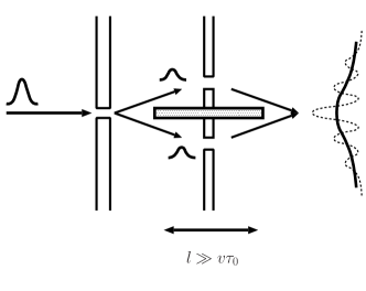
Figure 2: According to the modified dynamics, the interference fringe pattern due to split and recombined wave packets is predicted to be washed out, if the distinct wave packets in a superposition had been spatially separated further than their own widths for a duration longer than the collapse time $\tau_{0}$ before the recombination, e.g., if the length $l$ of the impenetrable partition slab separating the two paths is made larger than a coherence length $\sim v\tau_{0}$, where $v$ is the velocity of the incoming wave packet.

The modified dynamics describes the ‘measurement’ involving wave function collapse as a stochastic process to minimize $|\delta{\bf r}|$ of the wave function $\Psi$. It serves our purpose that those classically inadmissible superposition states of well separated wave packets like (24) are destabilized to decay with the finite lifetime $\tau_{0}$. In principle, the non-trivial physical effects of the model should be manifested themselves in the interference experiments which are devised to distinguish the pure state $\Psi$ from the statistical mixture of the collapse outcomes $\Phi_{n}$. For instance, we are led to an unconventional prediction of the destruction of the quantum interference pattern, as schematically presented in Fig. 2. Since such an intrinsic decoherence is concluded independently of the actual distance between the separated wave packets in superposition, we must also conclude seemingly unfavorable consequences for the microscopic single-particle states with nodes along which the density vanishes, $\rho({\bf r})=0$. In contrast to (20) for (19), e.g., the wave function $\phi_{\pi}({\bf r})\propto x\phi_{\sigma}({\bf r})$ for $\sigma\ll\lambda_{0}$ cannot but be halved to result in the effectively nodeless collapse outcomes $P_{\pm}\phi_{\pi}$;

$$\phi_{\pi}({\bf r})\longrightarrow\theta(\pm x)\phi_{\pi}({\bf r}),$$

as one obtains $\lambda\simeq\sigma^{3}/\lambda_{0}^{2}\ll\sigma$ in this case. In short, the modified dynamics predicts that wave functions with nodes generally have to be nodeless eventually. It is clear that such drastic unconventional collapse processes must not intervene the conventional Schrödinger time evolution too frequently. Thus we have to require the collapse time $\tau_{0}$ to be substantially slower than any practical coherence time scales for the quantum interference of spatially separated wave packets.

III.4 Numerical estimate of the model parameters

In practice, the numerical value for $T_{0}$ must be properly chosen such that the characteristic length $\lambda_{0}$ for microscopic particles like electron and neutron must be too large while the intrinsic wave packet widths $\lambda_{0}$ for macroscopic bodies, which may be effectively regarded as material points, are too small to be unexpectedly detected experimentally. To put it concretely, in order to guarantee $\lambda_{0}>10$m for electron while $\lambda_{0}<1\mu$m for a tiny particle of a nanogram, we estimate $10^{-49}\ {\rm J}<T_{0}<10^{-39}\ {\rm J}.$ Hence there is a relatively wide range open for $T_{0}$, owing to the above note that the model is relatively insensitive to $T_{0}$.

On the other hand, we must assume the collapse time $\tau_{0}$ to be larger than a typical coherence time scale of microscopic quantum phenomena, as mentioned in the last subsection. Nonetheless, at the same time, $\tau_{0}$ must be shorter than a typical scale of macroscopic classical phenomena in order to warrant definite outcomes for classical bodies approximately at any time, i.e., to prevent such an embarrassing superposition state of ‘classical’ states with ‘distinct’ spatial configurations from developing and lasting for a long while. Therefore one may make a rough estimate like $10^{-6}{\rm sec}\ll\tau_{0}\ll 10^{-1}{\rm sec}$, so we find that the parameter range allowed for $\tau_{0}$ is more restricted than $T_{0}$. In fact, we consider that whether we could assume $\tau_{0}$ properly would be the crucial point for the present model to be viable physically. In what follows, we discuss the implications of the model assuming that experiments do not exclude room for the model parameters.

Without being affected by the collapse, the wave packet evolves according to (1) for the duration of order $\tau_{0}$. In the meantime, the width $(\delta{\bf r})^{2}\simeq\lambda_{0}^{2}$ for a free particle grows up to $\lambda_{0}^{2}\left(1+(\frac{T_{0}\tau_{0}}{4\pi\hbar})^{2})\right)$, so that the second length scale must be introduced if $T_{0}\tau_{0}\gg 4\pi\hbar$. However, with the above estimate of $T_{0}$ taken for granted, this limit must be rejected physically, because we hardly accept $\tau_{0}$ as long as $\hbar/T_{0}>10^{5}$ second on physical grounds. Hence it is valid to use the single length scale (18) in free space, since we can consistently assume

$$T_{0}\tau_{0}\ll 4\pi\hbar$$ (26)

without invalidating the model.

IV Motion in one dimension

IV.1 Model

To give shape to the model, we investigate motion of a particle in one dimension. The unmodified Schrödinger equation may be written in a dimensionless form,

$${\rm i}\frac{\partial}{\partial\tilde{t}}\Psi=-\frac{\partial^{2}}{\partial\tilde{x}^{2}}\Psi+V(\tilde{x}),$$ (27)

where $\tilde{t}=T_{0}t/\hbar$ and $\tilde{x}=x/\lambda_{0}$. As discussed above, for macroscopic classical bodies, the potential $V(\tilde{x})$ should be slowly varying, $|\nabla V|\ll|V|$. In practice, the time scale $T_{0}/\hbar$ of (27) should be substantially slower than $\tau_{0}$, as noted in (26). Nevertheless, in this section, we assume $T_{0}\tau_{0}=\hbar$ and $\tilde{t}=t/\tau_{0}$, for simplicity, to illustrate how the probabilistic and deterministic time evolutions compete with each other.

It is generally difficult to evaluate the localization functions analytically for an arbitrarily given state (cf. Appendix A), so that we discuss only the simple case that the state $\Psi(x)$ is divided by collapse into the left and right halves at a position $x_{0}$. To describe the collapse, let us make use of the two trial functions for the localization functions as follows (cf. Fig. 8),

$$P_{L}^{x_{0}}(x)=\left\{\displaystyle\begin{array}[]{cc}1,&x-x_{0}\leq-2\lambda\\ \cos\frac{\pi}{8\lambda}{(x-x_{0}+2\lambda)},&|x-x_{0}|\leq 2\lambda\\ 0,&2\lambda\leq x-x_{0}\end{array}\right.$$ (28)

and

$$P_{R}^{x_{0}}(x)=\left\{\begin{array}[]{cc}0,&x-x_{0}\leq-2\lambda\\ \cos\frac{\pi}{8\lambda}{(x-x_{0}-2\lambda)},&|x-x_{0}|\leq 2\lambda\\ 1,&2\lambda\leq x-x_{0}\end{array}\right.$$ (29)

with which we obtain

$$\Delta E=\frac{1}{2m}\left(\frac{\pi\hbar}{8\lambda}\right)^{2}\int_{x_{0}-2\lambda}^{x_{0}+2\lambda}\rho(x){\rm d}x.$$ (30)

The entropy change is approximately given by

$$\Delta S\simeq-w_{R}\log w_{R}-w_{L}\log w_{L},$$ (31)

where

$$w_{L}=\int_{-\infty}^{\infty}(P_{L}^{x_{0}}(x))^{2}\rho(x){\rm d}x$$

and $w_{R}=1-w_{L}$ are the probabilities to result in $P_{L}^{x_{0}}\Psi$ and $P_{R}^{x_{0}}\Psi$, respectively.

In order to fix $x_{0}$ and $\lambda$, we have to evaluate $S^{\prime}$ in (6) for the given density $\rho(x)=|\Psi(x)|^{2}$ at every moment. Nevertheless, to reduce the numerical task, we assume to set $\lambda=\lambda_{0}/8$ arbitrarily, and choose $x_{0}$ so as to minimize $\Delta F\equiv\Delta E-T_{0}\Delta S$ with (31) in anticipation that the qualitative features shown below would not be severely modified by the assumption. In effect, we are interested in the interplay of the stochastic and deterministic evolution. In what follows, we set $\hbar=1$, while assuming $T_{0}=1$ and $\tau_{0}=1$ despite (26).

IV.2 Results

Figure 3: Time evolution of the wave packet density $\rho(x,t)$ of a free particle with $2m=1$, starting from the Gaussian $\Psi(x,0)\propto{\rm e}^{-(x/\delta)^{2}}$ with $\delta=\lambda_{0}/3$ (cf. $\lambda_{0}=3.5$). Without (left) and with (right) collapse. Two stochastic collapses are recognized. In our model, the intermittent collapses keep the wave packet from diffusing, while setting it in Brownian motion.

Figure 4: Quantum tunneling through a potential barrier at $x\simeq 0$. The density $\rho(x,t)$ of a particle with $m=1$ in motion, evolving from $\Psi(x,0)\propto{\rm e}^{-(x/\delta)^{2}+{\rm i}p_{0}x_{0}}$ with $\delta=\lambda_{0}/2$, $x_{0}=-8$ and $p_{0}=8$. The potential is $V(x)\simeq 0.08{\rm e}^{-4x^{2}}$. Without (left) and with (right) collapse. Two collapses before and after reflection(transmition) are recognized. Tunneling failed, and the wave packet is reflected. Aside from a digression over the barrier, the wave packet traces an approximately well-defined trajectory.

To begin with, we give results for a free particle, $V(x)=0$, in Fig. 3. Here and below, the results for the density $\rho(x,t)$ with and without collapse are compared with each other to make the non-trivial collapse effect clear. As shown by contours on the base ($x$-$t$ plane) of Fig. 3, the collapsing wave packet traces a zig-zag world line. To a greater or lesser extent, the discontinuity is a general and non-trivial feature to be revealed in our results. This is made conspicuous when we should otherwise, without collapse, get involved in a controversial superposition state. As a typical case, results for a moving particle impinging on a potential barrier at $x\sim 0$ are given in Fig. 4.

Figure 5: Quantum oscillation in a double well potential ($m=2$). Without (left) and with (right) collapse. There are potential walls at $x=\pm 1$, and a square potential of the width and the height of 0.1 at $x=0$. The sinusoidal continuous oscillation apparent in the left figure is suppressed by collapse. On the time scale of the figure, individual collapse are not conspicuous. In the right figure, we observe that the particle is found to be either in $x>0$ or $x<0$, instead of being in their superposition. The particle position changes discontinuously from time to time at random. In a conventional phrase, the particle behaves as if it is “measured” with the frequency $\gamma_{0}$.

Figure 6: Quantum decay of a particle $m=2$ trapped in a potential well. The potential well $-1\leq x<0$ is that of Fig. 5 with the wall at $x=1$ removed. Without (left) and with (right) collapse. The wave packet is literally trapped until it goes off at a definite, but unpredictable, instant.

Results for the system in a double well potential are shown in Fig. 5, for which we varied $x_{0}$ for fixed $\lambda=\lambda_{0}/16$, as the constraint allows the width $\lambda$ to be smaller in this case. We find that even $\lambda=\lambda_{0}/32$ does not change the results qualitatively, for the wave function tends to collapse around $x\simeq 0$. The suppression of a coherent quantum motion by frequent “measurements” is generally known as the quantum Zeno effectMisra and Sudarshan (1977); Peres (1980); Kraus (1980). This is demonstrated in Fig. 5. We are also interested in a related problem of quantum decay from a potential well. To realize such, we solved a simple model as indicated in Fig. 6. It is noted that the unstable state trapped in the potential barrier looks stationary until it decays spontaneously.

Figure 7: Quantum “measurement” caused by a time-dependent potential. A partition wall is adiabatically inserted at the center of a bound state ($2m=1$) in the potential well $-1\leq x\leq 1$. Without (left) and with (right) collapse taken account of. The potential is the same as in Fig. 5, except that the height of the central square potential is increased as $v_{\rm height}=0.1t$. The wave packet is finally found in either of the left or right partition.

Lastly, to mimic situations encountered in position measurement, wave packet reduction induced by a time-dependent potential is displayed in Fig. 7, which shows that gradual increase of the external potential may cause a sudden change of state. To obtain Fig. 7, we varied $\lambda$ for $x_{0}=0$. This behavior corresponds to the transition from (20) to (25). In general, we associate the “measurement” of a quantum particle with such an unordinary leap caused by a specially prepared external potential.

These results demonstrate that the effect of collapse becomes conspicuous when the linear width $\delta$ of the wave packet exceeds the characteristic length scale $\lambda_{0}$, and that the collapse hardly affects the wave packet when $\delta\ll\lambda_{0}$. Therefore, as discussed in the previous sections, we obtain a picture in that quantum (wave) mechanics obtains in the one limit $\lambda_{0}\rightarrow\infty$, while classical (particle) mechanics (with a definite path) emerges in the other limit $\lambda_{0}\rightarrow 0$.

V Discussion

According to the model, wave function reduction causes the density matrix of the pure state $\Psi({\bf r})$ to evolve as

$$\rho({\bf r},{\bf r^{\prime}})=\Psi({\bf r})\Psi^{*}({\bf r^{\prime}})\longrightarrow{\mit\Delta({\bf r},{\bf r^{\prime}})}\Psi({\bf r})\Psi^{*}({\bf r^{\prime}}),$$ (32)

where

$$\mit\Delta({\bf r},{\bf r^{\prime}})\equiv\sum_{n}P_{n}({\bf r})P_{n}^{*}({\bf r^{\prime}})$$ (33)

equals 1 for ${\bf r}={\bf r^{\prime}}$ because of (4), and vanishes for $|{\bf r}-{\bf r^{\prime}}|\gg\lambda$. Hence, by postulate, the diagonal elements $\rho({\bf r},{\bf r})=\rho({\bf r})$ are invariant upon collapse. As the functions $P_{n}$ are determined by $\rho({\bf r})$, so is $\mit\Delta({\bf r},{\bf r^{\prime}})$. Therefore, (32) generally represents a non-linear transformation. Nevertheless, in many practical cases, the localization functions may be determined by the external potential $V({\bf r})$, as in Figs. 5 and 7. In fact, this would be the case when we can neglect wave function collapse except in measurement-related situations. In such cases, we obtain a linear equation, referring to Fig. 1,

$$\rho_{t+{\rm d}t}=\left(1-\gamma_{0}{\rm d}t\right)\left(\rho_{t}+\frac{{\rm i}}{\hbar}[\rho_{t},H]_{-}{\rm d}t\right)+\gamma_{0}{\rm d}t\mit\Delta({\bf r},{\bf r^{\prime}})\rho_{t},$$

or

$$\frac{{\rm d}\rho}{{\rm d}t}=\frac{{\rm i}}{\hbar}[\rho,H]_{-}-\gamma_{0}\left(1-\mit\Delta\right)\rho.$$ (34)

The equation of motion (34) has the same form as that investigated by Joos and Zeh to assess the effect of decoherence through interaction with the environmentJoos and Zeh (1985).

At the statistical level of description, the collapse (32) does not affect the density matrix $\rho({\bf r},{\bf r}^{\prime})$ unless it has the longer ranged correlation than the correlation length $\lambda$ of (33). For example, for free particles in thermal equilibrium at temperature $T$, we have

$$\rho({\bf r},{\bf r^{\prime}})\simeq\lambda_{T}^{-3/2}\exp\left(-\frac{\pi|{\bf r}-{\bf r^{\prime}}|^{2}}{\lambda_{T}^{2}}\right),$$ (35)

where $\lambda_{T}$ is the thermal de Broglie wavelength at $T$. In order for (32) to affect the statistical results based on (35), we should assume $\lambda_{T}\gg\lambda_{0}$, or the physical temperature must be extremely low, $T\ll T_{0}$. Consequently, in the statistical ensemble, the phenomenological effects of collapse apparent at the individual level can be completely masked by environmental decoherenceGallis and Fleming (1990); Tegmark (1993); Giulini et al. (1996); Zurek (2003); Tessieri et al. (1995). In other words, the discontinuity due to collapse as indicated in Figs. 3 and 7 would be averaged out at the statistical level.

Last but not least, the theory discussed throughout the paper is essentially non-relativistic. This is evident from a special role we assigned to time $t$. It is still noteworthy that the model formulated with $\rho({\bf r})$ is Galilei invariant. The conflict of the instantaneous collapse with special relativity has been elucidatedAharonov and Albert (1981). In this regard, we only note a consistent if naive attitude to fit with the present model, that is, to assume a special frame of reference, as noted by EberhardEberhard (1978) and BellBell (1987b), in which the collapse dynamics applies specificallynot .

VI Conclusion

In this paper, we addressed ourselves to the problem of how the classical world as we experience it emerges from the underlying laws of quantum mechanics. We investigated the motion of a quantum particle on the basis of the proposed modified dynamics of wave function collapse. In effect, the proposal may look complicated in practice, owing to the task of solving for the localization functions, but the model is simple in principle, as summarized in Fig. 1. We describe the collapse dynamics in terms of physical quantities such as energy, entropy, and density in real space. The model contains two material-independent constants $\tau_{0}=\gamma_{0}^{-1}$ and $T_{0}$. It is suggested on the analogy of the second law of thermodynamics in order to destabilize those linear superpositions of spatially separated wave packets, which are hardly interpretable from an ordinary, classical, realistic standpoint. On the basis of the proposal, the numerical results are obtained as displayed in Figs. 3-7. The model reproduces classical mechanics as a limit, yet it does not use the classical limit for its own formulation. According to the model, we obtain a unified mechanical picture in that the classical picture emerges on a long and large scale, $t\gg\tau_{0}$ and $x\gg\lambda$, while the quantum picture applies in the opposite limits, $t\ll\tau_{0}$ and $x\ll\lambda$, where $\lambda$ denotes the natural linear dimension of the wave packet determined according to the model. In fact, the length scale $\lambda$ of collapse depends on circumstances, and it can be made arbitrarily small. This is particularly the case for a microscopic particle subjected to measurement-related situations, where one can devise an apparatus to make $\lambda$ as small as one likes, in principle.

Appendix A Variational Principle

In principle, it is possible to write down the equations for $P_{n}({\bf r})$, that is, the equations to determine the collapse outcome states $\Phi_{n}({\bf r})$. However, it is generally difficult to solve them for an arbitrary state $\Psi({\bf r})$ analytically. In this appendix, we investigate the simplest tractable case where a wave packet is justly halved with equal probability by collapse.

We obtain the localization functions $P_{1}$ and $P_{2}$ under the condition that the collapse probabilities to the two outcomes are equal, viz., $w_{1}=w_{2}=1/2$. To this end, the auxiliary function $\theta({\bf r})$, ranging from 0 to $\pi/2$, is introduced by $P_{1}=\cos\theta$ and $P_{2}=\sin\theta$ to take account of the constraint $P_{1}^{2}+P_{2}^{2}=1$. In general, the collapse outcomes $P_{n}\Psi$ are not orthogonal, or the overlap integral

$$p=\langle\Psi|P_{1}P_{2}|\Psi\rangle=\frac{1}{2}\int{\rm d}{\bf r}\rho({\bf r})\sin 2\theta({\bf r})$$ (36)

does not vanish. Hence the entropy production by the collapse is given by

$$\Delta S=-\left(\frac{1}{2}+p\right)\log\left(\frac{1}{2}+p\right)-\left(\frac{1}{2}-p\right)\log\left(\frac{1}{2}-p\right),$$

which takes the maximum value $\log 2$ for $p=0$, while the minimum is $\Delta S=0$ for $p=1/2$.

In order to achieve the localization of wave function, to maximize $\overline{\rho^{2}}$ in (14) is more easily implemented than to work with $(\delta{\bf r})^{2}$, (12). Hence, to start with, let us maximize

$$\overline{\rho^{2}}=2\int(\sin^{4}\theta+\cos^{4}\theta)\rho({\bf r})^{2}{\rm d}{\bf r}$$ (37)

under (7), for which

$$\Delta E=\frac{\hbar^{2}}{2m}\int\left(\nabla\theta\right)^{2}\rho({\bf r}){\rm d}{\bf r}.$$ (38)

In terms of a Lagrange multiplier $\lambda^{\prime}$, the equation for $\theta$ is obtained by the variation principle,

$$\frac{\delta}{\delta\theta}(\overline{\rho^{2}}+\lambda^{\prime}(T_{0}\Delta S-\Delta E))=0,$$

from which we obtain the equation

$$\lambda^{\prime}\left(\frac{\hbar^{2}}{m}\nabla(\rho\nabla\theta)-T_{0}\frac{\rho}{2}\log\frac{1+p}{1-p}\cos 2\theta\right)=2\rho^{2}\sin 4\theta.$$ (39)

In particular, we are interested in the case $p\simeq 0$ and $|\nabla\rho/\rho|\ll|\nabla\theta|$, where the model predicts the non-trivial result that the collapse outcomes $P_{1}\Psi$ and $P_{2}\Psi$ are distinctly different from each other, $\langle\Phi_{1}|\Phi_{2}\rangle\simeq 0$. To discuss this case further in depth, regarding $\theta$ as a function of $x$ for simplicity, we obtain the one-dimensional equation

$$4\lambda^{2}\frac{{\rm d}^{2}\theta}{{\rm d}x^{2}}=\sin 4\theta,$$ (40)

where $\lambda=\sqrt{\hbar^{2}\lambda^{\prime}/8m\rho}.$

The equation of a pendulum (40) can be solved analytically. The solution with a proper boundary condition is given by

$$\cos 2\theta=-{\rm sn}(x/\lambda,1)=-\tanh(x/\lambda),$$ (41)

where ${\rm sn}(u,k)$ is the Jacobian elliptic function. The origin of the $x$ axis has to be consistently chosen to give $w_{1}=w_{2}=1/2$, i.e., by

$$\int\tanh(x/\lambda)\rho{\rm d}{\bf r}=0.$$ (42)

The solution (41) for $\lambda=1$ is shown in Fig. 8 with the solid curve. Note that the curve essentially represents the localization function $P_{2}(x)^{2}$, because

$$P_{1,2}(x)^{2}=\frac{1\pm\cos 2\theta}{2}.$$

To estimate the energy cost (38) to fix $\lambda$, we can make use of ‘energy conservation’ of the pendulum motion (40),

$$8\lambda^{2}\left(\frac{{\rm d}{\theta}}{{\rm d}x}\right)^{2}+V(\theta)=V(0),$$ (43)

where

$$V(\theta)=\frac{1}{4}\cos 4\theta.$$ (44)

From the last equations, we obtain

$$4\lambda^{2}\left(\frac{{\rm d}{\theta}}{{\rm d}x}\right)^{2}=P_{1}(x)^{2}P_{2}(x)^{2},$$

hence,

$$\Delta E=\frac{\hbar^{2}q}{8m\lambda^{2}},$$ (45)

where

$$q=\int P_{1}^{2}(x)P_{2}^{2}(x)\rho{\rm d}{\bf r}\simeq\int{\rm e}^{-x^{2}/\lambda^{2}}\rho{\rm d}{\bf r}.$$ (46)

With respect to the last approximation, we should note $\int P_{1}(x)^{2}P_{2}(x)^{2}{\rm d}x=2\lambda$, while $\int{\rm e}^{-x^{2}/\lambda^{2}}{\rm d}x=\sqrt{\pi}\lambda$, and $P_{1}(x)^{2}P_{2}(x)^{2}\simeq{\rm e}^{-x^{2}/\lambda^{2}}\simeq 1-(x/\lambda)^{2}$ for $|x|\ll\lambda$. Similarly, we may write (36) as

$$p\simeq\int{\rm e}^{-x^{2}/2\lambda^{2}}\rho{\rm d}{\bf r},$$ (47)

with which $\rho({\bf r})=|\Psi({\bf r})|^{2}$ must meet $p\ll 1$ as well as (42) for consistency. Given such $\rho({\bf r})$, the parameter $\lambda$ for $P_{n}({\bf r})$ is determined by $\Delta E\simeq T_{0}\log 2$, as in (22). In consequence, we obtain the collapse outcomes $\Phi_{n}=\sqrt{2}P_{n}\Psi$. Note in particular that $P_{n}$ becomes the step function in the limit $\lambda\rightarrow 0$, e.g., as a result of the low density at $x=0$, $\rho(x=0)\simeq 0$. Then we recover the Born’s-rule probabilities $w_{n}=|\langle\Phi_{n}|\Psi\rangle|^{2}$ together with the non-overlapping collapse outcomes $\Phi_{n}$, owing to $P_{n}^{2}\simeq P_{n}$. As is clear from the qualitative discussion in Section III.2, this feature is generic and not specific to the assumption $w_{1}=w_{2}$.

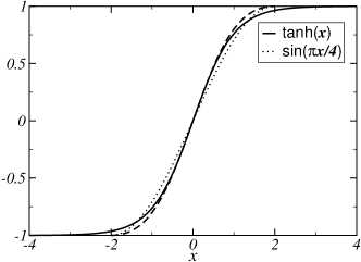
Figure 8: The localization function $2P_{2}(x)^{2}-1=-\cos 2\theta$ is shown as a function of $x$. The solid and dashed curve are the solutions of (40) and (48) for $\lambda=1$, respectively. The dotted curve is a sine curve, which is added for reference.

In a similar manner, we can fix $P_{n}$ by maximizing (6) instead of $\overline{\rho^{2}}$, (37). To obtain $\Phi_{n}$ from $\Psi$, our task is to maximize

$$S^{\prime}+\beta(T_{0}\Delta S-\Delta E),$$

where $E={\rm Tr}(\hat{\rho}\hat{H})$, $S=-{\rm Tr}(\hat{\rho}\log\hat{\rho})$, and $\beta$ is the Lagrange multiplier to keep the postulated constraint $\Delta(E-T_{0}S)=0$. In the same approximations as above, in place of (40), we obtain

$$4\lambda^{2}\frac{{\rm d}^{2}\theta}{{\rm d}x^{2}}=\sin 2\theta\log\cot\theta,$$ (48)

where $4\lambda^{2}={\hbar^{2}}\beta/{m}$. A numerical solution $\cos 2\theta$ for $\lambda=1$ is shown in Fig. 8 with the dashed curve. We find that the optimal shape of the localization function $P_{n}(x)$ is not severely modified. For reference, a sinusoidal function $\sin\pi x/4$ for $|x|\leq 2$ is also shown in Fig. 8 with the dotted curve.

It is noted that the solution of (48) gives a finite value for $|x(\theta=\pi/2)-x(\theta=0)|$, which is the overlap width of $P_{1}(x)P_{2}(x)$. This is because the ‘potential’ $V(\theta)=(\log\sin(2\theta)+\cos(2\theta)\log\cot\theta)/2$ for (48) makes the integral

$$\int_{0}^{\pi/2}\frac{{\rm d}\theta}{\sqrt{V(0)-V(\theta)}}$$

convergent, while (44) makes this expression divergent. Thus we obtain compact support of $\Phi_{n}$, which is a favorable feature of the model. Moreover, from (43), we obtain $|{\rm d}\theta/{\rm d}x|\rightarrow 0$ as $\theta\rightarrow 0,\pi/2$ for the solution of (48), by which follows the continuity of $\Phi_{n}(x)$ as well as their derivatives as a function of $x$. Furthermore, as discussed below, the expression (6) is generalized adequately to describe independent collapse of many particle systems.

Appendix B Generalization to Many-particle systems

In the main text, we focused on single-particle problems of the modified dynamics. To describe collapse of a many particle system, we have to generalize the localization functions to $P_{n}({\bf r}_{1},{\bf r}_{2},\cdots,{\bf r}_{N})$, which are to be multiplied with the $N$ particle wave function $\Psi({\bf r}_{1},{\bf r}_{2},\cdots,{\bf r}_{N})$. Accordingly, the integral $\int{\rm d}{\bf r}$ in (3) is generalized to $\int{\rm d}{\bf r}_{1}{\rm d}{\bf r}_{2}\cdots{\rm d}{\bf r}_{N}$ over $3N$ dimensional space for the $N$ particles.

For $N$ distinguishable particles, one should maximize

$$S^{\prime}=\sum_{n}w_{n}\int|\Phi_{n}|^{2}\log|\Phi_{n}|^{2}{\rm d}{\bf r}_{1}{\rm d}{\bf r}_{2}\cdots{\rm d}{\bf r}_{N},$$ (49)

instead of (6). In particular, when the $N$ particles are independent from each other, the wave function of the whole system is represented by the product of wave functions,

$$\Psi({\bf r}_{1},{\bf r}_{2},\cdots,{\bf r}_{N})=\prod_{i=1}^{N}\psi_{i}({\bf r}_{i}).$$

for which one can regard formally that each of the states $\psi_{i}({\bf r}_{i})$ collapses independently,

$$\psi_{i}\rightarrow\phi_{n_{i}}=\frac{1}{\sqrt{w_{n_{i}}}}P_{n_{i}}\Psi_{i},$$

since (49) is decomposed into a sum of $N$ independent terms,

$$S^{\prime} = \sum_{i=1}^{N}\sum_{n_{i}}w_{n_{i}}\int|\phi_{n_{i}}|^{2}\log|\phi_{n_{i}}|^{2}{\rm d}{\bf r}_{i},$$

owing to $w_{n}=\prod_{i}w_{n_{i}}$. This is a feature to be expected physically.

For indistinguishable particles, the symmetry of the wave function $\Psi$ must be respected, so that the localization functions $P_{n}({\bf r}_{1},{\bf r}_{2},\cdots,{\bf r}_{N})$ must be symmetric under the exchange of the arguments. For definiteness, they are approximately given in terms of $P_{n}({\bf r})$ for a single particle state as follows. The simplest assumption is to regard them simply as functions of the center-of-mass coordinate ${\bf R}=\sum_{i}{\bf r}_{i}/N$,

$$P_{n}({\bf r}_{1},{\bf r}_{2},\cdots,{\bf r}_{N})=P_{n}({\bf R}).$$

Otherwise, they may be represented as symmetrized products of $P_{n}({\bf r})$,

$$P_{n}({\bf r}_{1},{\bf r}_{2},\cdots,{\bf r}_{N})^{2}=\sum P_{n_{1}}({\bf r}_{1})^{2}P_{n_{2}}({\bf r}_{2})^{2}\cdots P_{n_{N}}({\bf r}_{N})^{2},$$

where $n$ represents a set of integers $(n_{1},n_{2},....,n_{N})$ and the sum in the right-hand side is taken over all different permutations of them, so that

$$\sum_{n}P_{n}^{2}=\prod_{i=1}^{N}\left(\sum_{n_{i}}P_{n_{i}}({\bf r}_{i})^{2}\right)=1.$$

For identical particles, the following expression may equally serve our purpose,

$$S^{\prime}=\sum_{n}w_{n}\int\rho_{n}({\bf r})\log\rho_{n}({\bf r}){\rm d}{\bf r},$$ (50)

where $\rho_{n}({\bf r})=\langle\Phi_{n}|\hat{n}_{\bf r}|\Phi_{n}\rangle$ denotes the particle density in terms of the number operator $\hat{n}_{\bf r}$. In any case, the $N$ identical particles must evolve simultaneously as $\Psi\rightarrow P_{n}\Psi/{\sqrt{w_{n}}},$ as they are not strictly independent from each other.

To treat the case where the particle number $N$ is variable, we have to generalize the collapse prescription furthermore to realize the localization on the number basis as well. This is not difficult in principle, but goes beyond the scope of the paper.

References

- Cohen-Tannoudji and Dalibard (1986) C. Cohen-Tannoudji and J. Dalibard, Europhys. Lett. 1, 441 (1986).
- Poratti and Putterman (1987) M. Poratti and S. Putterman, Phys. Rev. A 36, 929 (1987); M. Poratti and S. Putterman, Phys. Rev. A 39, 3010 (1989).
- Sauter et al. (1986) T. Sauter, R. Blatt, W. Neuhauser, and P. E. Toschek, Opt. Commun. 60, 287 (1986).
- Cook (1988) R. Cook, Phys. Scr. T21, 49 (1988).
- Blatt and Zoller (1988) R. Blatt and P. Zoller, Eur. J. Phys. 9, 250 (1988).
- Pegg and Knight (1988) D. T. Pegg and P. L. Knight, A37, 4303 (1988).
- Ambrose and Moerner (1991) W. P. Ambrose and W. E. Moerner, Nature 349, 225 (1991).
- Ralls and Buhrman (1988) K. S. Ralls and R. A. Buhrman, Phys. Rev. Lett. 60, 2434 (1988).
- Bergquist et al. (1986) J. C. Bergquist, R. G. Hulet, W. M. Itano, and D. J. Wineland, Phys. Rev. Lett. 57, 1699 (1986).
- Nagourney et al. (1986) W. Nagourney, J. Sandberg, and H. Dehmelt, Phys. Rev. Lett. 56, 2797 (1986).
- Leibfried et al. (2003) D. Leibfried, R. Blatt, C. Monroe, and D. Wineland, Rev. Mod. Phys. 75, 281 (2003).
- Bohm (1952a) D. Bohm, Phys. Rev. 85, 166 (1952a); D. Bohm, Phys. Rev. 85, 180 (1952b); D. Bohm and B. Hiley, Phys. Rep. 172, 93 (1989).
- Holland (1993) P. Holland, The Quantum Theory of Motion (Cambridge University Press, 1993).
- Dürr et al. (1992) D. Dürr, S. Goldstein, and N. Zanghì, J. Stat. Phys. 67, 843 (1992).
- Ballentine (1970) L. E. Ballentine, Rev. Mod. Phys. 42, 358 (1970).
- Zeh (1970) H. Zeh, Found. Phys. 1, 77 (1970).
- Machida and Namiki (1980a) S. Machida and M. Namiki, Prog. Theor. Phys. 63, 1457 (1980a); S. Machida and M. Namiki, Prog. Theor. Phys. 63, 1833 (1980b).
- Joos and Zeh (1985) E. Joos and H. Zeh, Zeit. Phys. B 59, 223 (1985).
- Namiki and Pascazio (1993) M. Namiki and S. Pascazio, Phys. Rep. 232, 301 (1993).
- Giulini et al. (1996) D. Giulini, E. Joos, C. Kiefer, J. Kumpsch, I.-O. Stamatescu, and H. Zeh, Decoherence and the Appearance of a Classical World in Quantum Theory (Springer-Verlag, 1996).
- Zurek (2003) W. Zurek, Rev. Mod. Phys. 75, 715 (2003).
- van Frassen (1991) B. van Frassen, Quantum Mechanics: an Empiricist View (Clarendon Press, Oxford, 1991).
- Healey (1989) R. Healey, The Philosophy of Quantum Mechanics: an Interactive Interpretation (Cambridge University Press, 1989).
- Vermaas and Dieks (1998) P. Vermaas and D. Dieks, The Modal Interpretation of Quantum Mechanics (Kluwer Academic Publishers, Dordrecht, 1998).
- Griffiths (1984) R. Griffiths, J. Stat. Phys. 36, 219 (1984); R. Griffiths, Phys. Rev. A 54, 2759 (1996).
- Omnès (1992) R. Omnès, Rev. Mod. Phys. 64, 339 (1992).
- Gell-Mann and Hartle (1990) M. Gell-Mann and J. Hartle, in Complexity, Entropy, and the Physics of Information, edited by W.H.Zurek (Addison Wesley Publishing Company, Reading, 1990).
- Everett III (1957) H. Everett III, Rev. Mod. Phys. 29, 454 (1957).
- DeWitt and Graham (1973) D. DeWitt and N. Graham, The Many-Worlds Interpretation of Quantum Mechanics (Princeton University Press, 1973).
- Deutsch (1985) D. Deutsch, Int. Journ. Theor. Phys. 24, 1 (1985).
- Albert and Loewer (1988) D. Albert and B. Loewer, Synthese 77, 195 (1988).
- Albert (1992) D. Albert, Quantum Mechanics and Experience (Harward University Press, Cambridge, MA, 1992).
- Bell (1981) J. Bell, in Quantum Gravity 2, edited by C. Isham, R. Pensrose, and D. Sciama (1981), also in: Speakable and unspeakable in quantum mechanics, Cambridge University Press, 117 (1987).
- Bell (1990) J. Bell, in Sixty-Two Years of Uncertainity, edited by A. Miller (Plenum Press, New York, 1990), also in, Physics World 3, 33 (1990).
- Bohm and Bub (1966) D. Bohm and J. Bub, Rev. Mod. Phys. 38, 453 (1966).
- Pearle (1976) P. Pearle, Phys. Rev. D 13, 857 (1976); P. Pearle, Phys. Rev. Lett. 53, 1775 (1984); P. Pearle, Phys. Rev. A 39, 2277 (1989).
- Diósi (1985) L. Diósi, Phys. Lett. A 112, 288 (1985); L. Diósi, Phys. Lett. A 122, 221 (1987); L. Diósi, Phys. Lett. A 129, 419 (1988).
- Gisin (1984a) N. Gisin, Phys. Rev. Lett. 52, 1657 (1984a); N. Gisin, Phys. Rev. Lett. 53, 1776 (1984b).
- Ghirardi et al. (1986) G. C. Ghirardi, A. Rimini, and T. Weber, Phys. Rev. D34, 470 (1986).
- Bell (1987a) J. Bell, in Schrödinger: Centanary Celebration of a Polymath, edited by C. Kilmister (Cambridge University Press, Cambridge, 1987a), also in, Speakable and unspeakable in quantum mechanics, Cambridge University Press, 201 (1987).
- Ghirardi et al. (1990) G. Ghirardi, P. Pearle, and A. Rimini, Phys. Rev. A 42, 78 (1990).
- Ghirardi (2000) G. Ghirardi, Found. Phys. 30, 1337 (2000).
- Bassi and Ghirardi (2003) A. Bassi and G. Ghirardi, Phys. Rep. 379, 257 (2003).
- Pearle (1999) P. Pearle, in Open Systems and Measurement in Relativistic Quantum Theory, edited by F.Petruccione and H.P.Breuer (Springer Verlag, 1999).
- Pearle et al. (1999) P. Pearle, J. Ring, J. I. Collar, and F. T. Avignone III, Found. Phys. 29, 465 (1999).
- Frenkel (1990) A. Frenkel, Found. Phys. 20, 159 (1990).
- Milburn (1991) G. J. Milburn, Phys. Rev. A44, 5401 (1991).
- Percival (1995) I. C. Percival, Proc. R. Soc. Lond. A451, 503 (1995).
- Hughston (1996) L. Hughston, Proc. R. Soc. London A 452, 953 (1996).
- Adler and Howritz (2000) S. Adler and P. Howritz, J. Math. Phys. 41, 2485 (2000); S. Adler and T. Brun, J. Phys. A 34, 4797 (2001); S. Adler, J. Phys. A 35, 841 (2002).
- (51) A preliminary version of the work is to appear in Opt. Spectr.; T. Okabe, quant-ph/0410095.
- Tegmark (1993) M. Tegmark, Found. Phys. Lett. 6, 571 (1993).
- Tessieri et al. (1995) L. Tessieri, D. Vitali, and P. Grigolini, Phys. Rev. A51, 4404 (1995).
- Misra and Sudarshan (1977) B. Misra and E. Sudarshan, J. Math. Phys. 18, 756 (1977).
- Peres (1980) A. Peres, Am. J. Phys. 48, 931 (1980).
- Kraus (1980) K. Kraus, Found. Phys. 11, 547 (1980).
- Gallis and Fleming (1990) M. R. Gallis and G. N. Fleming, Phys. Rev. A42, 38 (1990).
- Aharonov and Albert (1981) Y. Aharonov and D. Albert, Phys. Rev. D 24, 359 (1981); Y. Aharonov and D. Albert, Phys. Rev. D 29, 228 (1984).
- Eberhard (1978) P. Eberhard, Nuovo Cimento B 46, 392 (1978).
- Bell (1987b) J. Bell, in Speakable and unspeakable in quantum mechanics (Cambridge University Press, 1987b), p. 173.
- (61) Then the special frame would be experimentally distinguishable by a dilation of the collapse time .