Collapses and revivals of exciton emission in a semiconductor
microcavity: detuning and phase-space filling effects

Abstract

We investigate exciton emission of quantum well embedded in a semiconductor microcavity. The analytical expressions of the light intensity for the cases of excitonic number state and coherent state are presented by using secular approximation. Our results show that the effective exciton-exciton interaction leads to the appearance of collapse and revival of the light intensity. The revival time is twice compared the coherent state case with that of the number state. The dissipation of the exciton-polariton lowers the revival amplitude but does not alter the revival time. The influences of the detuning and the phase-space filling are studied. We find that the effect of the higher-order exciton-photon interaction may be removed by adjusting the detuning.

I Introduction

With the development of crystal growth techniques, people now can fabricate multi-dimensional confined nanostructure materials, such as quantum wells, quantum lines and quantum dots. Some interesting phenomena not observed in bulk material may take place within these systems. The optical properties of microcavity containing semiconductor quantum wells have been studied intensively in the recent years [1] since the first observation of polaritons splitting in strong-coupling regime [2]. The concept of the exciton-polariton was originally proposed by Hopfield [3]. In an infinite bulk crystals, the exciton is dressed by a photon with the same wave vector to form stable polariton due to the transitional symmetry of the total system.

It was shown that, for sufficiently small decay rates $\gamma_{ex}$ of the excitons and $\gamma_{c}$ of the photons, the coherent exciton-photon interaction gives rise to a periodic exchange of energy between the exciton and the photon modes. Therefore, the emission from the microcavity will show Rabi-like oscillating behavior [4, 5, 6, 7]. By regarding the excitons as a boson (i.e, harmonic approximation) and neglecting exciton-exciton interaction, i.e., within the completely linear regime, theoretical calculation of the light intensity gave a good agreement with the observed time-domain emission from the microcavity [5, 8]. Other effects, such as disorder-induced inhomogeneous broaden of the excitons [9] and the influence of squeeze vacuum of the photons [10] were also shown to have a strong influence on coherent dynamics of the exciton-photon coupling in microcavities.

Besides the coherent interaction between the excitons and the photons, nonlinear interaction between the excitons may play an indispensable role on the coupled exciton-photon system. In fact, the harmonic approximation is valid for the case that the exciton density is much lower than the Mott density, i.e., $n_{ex}a_{ex}^{3}\leq 10^{-2}$, where $n_{ex}$ is the exciton density and $a_{ex}$ is the two-dimensional Bohr radius. If the exciton density becomes relative higher, the ideal bosonic model of the excitons is no longer adequate. In this case, some residual Coulomb interactions among excitons and the phase-space filling effect should be taken into account [11]. It is well known that these complex nonlinear interactions lead to parametric amplification of an incident light from the microcavity [12, 13, 14, 15].

In Refs. [16, 17, 18], the authors studied the effect of the nonlinear interactions on the fluorescence spectrum of excitons. The deviation of high density excitons from the ideal boson model was investigated by introducing the concept of q-deformed excitons [17]. With the achivements of previous works mentioned above, it is natural to ask the effects of the exciton-exciton interaction on the light intensity from the semiconductor microcavity. Our previous work shows that the nonlinear interaction will lead to the appearance of collapses and revivals (CRs) in the light intensity [19]. Compared the initial coherent state case with the number state case, the revival time is twice. However, in our obtaining the simple but interesting relation, we ignored some important effects, such as the effects of the quantum dissipation processes, the higher-order exciton-photon interaction and the detuning between the exciton and photon modes.

In this paper, we study further the coherent dynamics of the coupled exciton-photon system in the semiconductor microcavities. The effects not considered in our previous paper will be taken into account. We would like to answer the following two questions: (1) does the relation of double revival time still hold after the consideration of these effects? (2) how can we keep the relation. This paper is ranged as the following: in section II, we give a general theoretical model of the interaction between a single-mode cavity field and the exctions. We present the approximate time-evolution operators by using the so-called secular approximation. In section III, the time-evolution of light intensity is calculated for the case the excitons are initially in a number state (or coherent state) and the photons are in vacuum. Finally, a brief summary and conclusion are presented in section IV.

II Theoretical Model

The considered system is a microcavity containing a semiconductor quantum well embedded in a high finesse cavity. We assume that the cavity and the quantum well are ideal, and they are in an extremely low temperature circumstance. The quantum well interacts with cavity field via exciton, which is an electron-hole pair bound by the Coulomb interaction. The exciton and the photon modes are quantized along the direction normal to the microcavity. We will consider the lowest-order mode in this direction. The excitons with in-plane wave vector ${\bf K}$ may only be dressed by the photons with the same wave vector due to the transitional invariance in the plane of the microcavity .

To further simplify the model, in this paper we will consider only one mode of photons with wave vector ${\bf K}=0$ and frequency $\omega_{c}$ very close to the lowest $n=1s$ exciton energy level [11, 20]. In fact, at extremely low temperature, the thermal momentum of the excitons is so small that the thermalized excitons can be neglected [17, 18]. Combining the above considerations and neglecting the spin degrees of freedom, one can write an effective interaction Hamiltonian for the coupled exciton-photon system as [11, 20]:

$$H = H_{0}+H_{NL}$$ (1)

$$= \omega_{c}a^{\dagger}a+\omega_{ex}b^{\dagger}b+g(a^{\dagger}b+b^{\dagger}a)$$ (3)

$$+Ab^{\dagger}b^{\dagger}bb-B\left(b^{\dagger}b^{\dagger}ba+a^{\dagger}b^{\dagger}bb\right),$$

where $b^{\dagger}(b)$ are creation (annihilation) operators of the excitons with frequency $\omega_{ex}$, and $a^{\dagger}(a)$ are the creation (annihilation) operators of the cavity field. We assume that both of them obey the bosonic commutation relation $[b,b^{\dagger}]=[a,a^{\dagger}]=1$. The third term stands for the exciton-photon interaction with coupling strength $g$, which is larger than nonlinear interaction coefficients $A$ and $B$. The fourth term describes the effective exciton-exciton interaction due to Coulomb interaction. The higher-order exciton-photon interaction, the fifth term, represents the phase-space filling effects. For small in-plane wave vectors of the excitons and the photons, the nonlinear interaction constants $2A=6Ry_{ex}a_{ex}^{2}/S$ and $B=g/\left(n_{sat}S\right)$, where $Ry_{ex}$ is the binding energy of the excitons, $S$ the quantization area and $n_{sat}=7/\left(16\pi a_{ex}^{2}\right)$ is the exciton saturation density [13, 21]. The ratio of the exciton-exciton interaction constant $A$ and the phase-space filling factor $B$ may be determined by a degenerate four-wave mixing experiment [22, 23]. In this paper, we assume that these two parameters are real and positive.

The dynamical evolution of the two-mode boson system described by Eq. (3) can not be calculated in an exact way due to the presence of nonlinear interaction $H_{NL}$. Some approximations will be involved in theoretical calculations. In Ref. [17, 18], the eigenvectors and eigenvalues of the total Hamiltonian (3) were solved by using first-order perturbation calculations. Recently, we restudied the dynamics of the total system by using unperturbation calculations [19], in which, however, the effects of the phase-space filling terms and the detuning between the cavity mode and the exciton eigenmode were not included at that time. In this paper, both the terms mentioned above and quantum dissipation processes due to the coupling with a continuum phonon mode will be taken into accounted.

Note that the linear part of Hamiltonian (3) may be diagonized by introducing two polariton operators:

$$p_{1}(t) = -va(t)+ub(t)\text{, }$$ (4)

$$p_{2}(t) = ua(t)+vb(t),$$ (5)

where $u$ and $v$ are Hopfield coefficients for the exciton and cavity modes, respectively. We assume that the coefficients are real and positive. The requirement of canonical transformations of Eq. (5) yields $u^{2}+v^{2}=1$, that is

$$[p_{i},p_{j}^{\dagger}]=\delta_{i,j}\text{, for }i\text{, }j=1\text{, }2\text{.}$$ (6)

The inverse transformations of Eq. (5) are

$$b(t) = up_{1}(t)+vp_{2}(t)\text{, }$$ (7)

$$a(t) = up_{2}(t)-vp_{1}(t).$$ (8)

Substituting Eq. (8) into the linear parts of Hamiltonian (3), we get

$$H_{0}=\sum_{j=1,2}\omega_{j}p_{j}^{\dagger}p_{j},$$ (9)

where

$$\omega_{j}=\frac{1}{2}\left[\omega_{ex}+\omega_{c}+(-1)^{j}\Delta\right]\text{, for }j=1\text{, }2\text{,}$$ (10)

are the lower-branch ($j=1$) and upper-branch ($j=2$) polariton energies, respectively, and $\Delta=\omega_{2}-\omega_{1}=\sqrt{\delta^{2}+4g^{2}}$ is the splitting energy of the two polaritons. The detuning between the cavity mode and the exciton mode is $\delta=\omega_{c}-\omega_{ex}$. In Eq. (9), we have let

$$\delta uv=g(u^{2}-v^{2}),$$ (11)

to cancel the nondiagonal terms in $H_{0}$. This condition plus the requirement of the canonical transformations of $p_{j}$ inspire us to define

$$u=\sin\theta\text{, }v=\cos\theta,$$ (12)

and tan$2\theta=-2g/\delta$. Substituting Eq. (8) into the nonlinear parts of Hamiltonian (3), one can obtain the effective polariton-polariton interaction term. Therefore, we may write the total Hamiltonian (3) in terms of the polariton operators as

$$H_{eff} = \sum_{j=1,2}\omega_{j}p_{j}^{\dagger}p_{j}+A_{11}p_{1}^{\dagger}p_{1}^{\dagger}p_{1}p_{1}$$ (14)

$$+A_{22}p_{2}^{\dagger}p_{2}^{\dagger}p_{2}p_{2}+2A_{12}p_{1}^{\dagger}p_{2}^{\dagger}p_{2}p_{1},$$

where

$$A_{11} = u^{3}\left(Au+2Bv\right)\text{, }A_{22}=v^{3}\left(Av-2Bu\right),$$ (15)

$$A_{12} = A_{21}=2uv\left[Auv-B\left(u^{2}-v^{2}\right)\right].$$ (16)

In Hamiltonian (14), we have neglected some terms proportional to $p_{1}^{\dagger}p_{1}^{\dagger}p_{2}p_{2}$, $p_{1}^{\dagger}p_{1}^{\dagger}p_{1}p_{2}$ and their Hermitian conjugate terms, which describe scattering processes between the two polariton branches and destroy particle-number conservation within each polariton branch. For the case of strong-coupling with the relative larger $g$, the energy gap $\Delta$ between the two polariton branches becomes larger, so one may safely adopt the so-called secular approximation [20, 24] to ignore the particle-number-nonconservation scattering channels. In some Refs.[25, 26], the authors calculated dynamics of a two-component Bose-Einstein condensate system by using the so called rotating-wave approximation (RWA). Physically, the essence of RWA is the same with the secular approximation, which is valid in the regime of weakly nonlinearity [24, 19], i.e., $A\text{, }B\ll g$.

From Hamiltonian (14), one may find that the polariton number operators $p_{j}^{{\dagger}}(t)p_{j}(t)$ of each branch are the constant of motion, i.e., $p_{j}^{{\dagger}}(t)p_{j}(t)=p_{j}^{{\dagger}}(0)p_{j}(0)=\text{const}$. Thus, the total particle number operator $N=\sum_{j}p_{j}^{{\dagger}}p_{j}=a^{\dagger}a+b^{\dagger}b$ is also time-independent. The formal solutions of the Heisenberg equations for the polariton operators $p_{j}(t)$ are

$$p_{j}(t) = \exp\left\{-i\left[\omega_{j}-i\gamma_{j}/2+2\sum_{k=1}^{2}A_{jk}p_{k}^{{\dagger}}p_{k}\right]t\right\}p_{j},$$ (17)

where $\gamma_{1}$ ($\gamma_{2}$) is the natural linewidth of the lower- (upper-) branch of the polariton [13]. These two parameters can be measured in the reflectivity spectrum of the microcavity[27]. In Eq. (17), the initial time operators (say, $p_{j}(0)$) have been written in the compact form ($p_{j}$). From now on, unless we specify otherwise, all the compact form operators stand for the operators at $t=0$. Although $p_{j}(t)$ and its Hermitian conjugate contain time-independent products $p_{k}^{{\dagger}}p_{k}$, the solutions of some measurable quantities are not trivial. In the following of this paper we will devote ourself to calculate the light intensity. Some novel physical results will be presented.

III Collapse and revival of the exciton-polariton emission

The oscillating emission from the microcavity had been demonstrated [5, 6]. The theoretical calculation of the light intensity by using the harmonic approximation gave a good agreement with the observed time-domain emission from the microcavity [5]. In our previous paper [19], we shown that the influence of the nonlinear exciton-exciton interaction may result in collapse and revival of the light intensity. In this section we will continue our calculations to study the effects of detuning, phase-space filling and quantum dissipation processing on the light intensity.

For a given initial state $|\psi(0)\rangle$ of the system, the intensity of the light field $I_{c}(t)=\langle\psi(0)|a^{\dagger}(t)a(t)|\psi(0)\rangle$ can be obtained as

$$I_{c}(t) = u^{2}\langle p_{2}^{\dagger}p_{2}\rangle+v^{2}\langle p_{1}^{\dagger}p_{1}\rangle-uv\left[\langle p_{1}^{\dagger}(t)p_{2}(t)\rangle+c.c\right],$$ (18)

where $\langle...\rangle=\langle\psi(0)|...|\psi(0)\rangle$. The initial state of the exciton-photon system is assumed as $|\psi(0)\rangle=\left|\phi(0)\right\rangle_{ex}\otimes\left|0\right\rangle_{c}$, i.e., the photons are initially in vacuum state. From Eq. (18), we find that only the last term is time-dependent so we need to calculate $\langle p_{1}^{\dagger}(t)p_{2}(t)\rangle$. With help of Eq. (17), we obtain

$$\langle p_{1}^{\dagger}(t)p_{2}(t)\rangle = e^{-2i(A_{11}-A_{22})t}e^{i(\omega_{1}-\omega_{2})t}e^{-(\gamma_{1}+\gamma_{2})t/2}$$ (20)

$$\times\left\langle e^{2i(A_{11}-A_{12})p_{1}^{\dagger}p_{1}t}p_{1}^{\dagger}p_{2}e^{2i(A_{12}-A_{22})p_{2}^{\dagger}p_{2}t}\right\rangle$$

$$= -e^{2i(A_{11}-A_{22})(\langle N\rangle/2-1)t}e^{i(\omega_{1}-\omega_{2})t}e^{-(\gamma_{1}+\gamma_{2})t/2}$$ (22)

$$\times\left\langle e^{-2i\theta J_{y}}e^{2i(A_{12}-A_{11})J_{z}t}J_{-}e^{2i(A_{12}-A_{22})J_{z}t}e^{2i\theta J_{y}}\right\rangle,$$

where $\langle N\rangle$ is the initial excitation number in the microcavity and $\theta$ is defined in Eq. (12). In Eq. (22), we have introduced the Schwinger’s angular momentums: $J_{z}=\frac{1}{2}(b^{\dagger}b-a^{\dagger}a)$ and the ladder operator $J_{+}=\left(J_{\_}\right)^{\dagger}=b^{\dagger}a$, so

$$p_{j}^{\dagger}p_{j} = N/2+(-1)^{j}e^{-2i\theta J_{y}}J_{z}e^{2i\theta J_{y}},$$ (23)

$$p_{1}^{\dagger}p_{2} = -e^{-2i\theta J_{y}}J_{-}e^{2i\theta J_{y}},$$ (24)

where the total particle number operator $N$ commutes with the introduced angular momentum operators $J_{\nu}$ ($\nu=x,y,z$). In the derivation of the final form of Eq. (22), we have also used a relation

$\displaystyle e^{2i\theta J_{y}}\exp\left[\lambda e^{-2i\theta J_{y}}J_{z}e^{2i\theta J_{y}}\right]e^{-2i\theta J_{y}}=\exp\left[\lambda J_{z}\right].$After the introduction of the angular momentum operators, any quantum states of the coupled exciton-photon system can be written in terms of the angular momentum states $|j,m\rangle=\frac{(b^{\dagger})^{j+m}(a^{\dagger})^{j-m}}{\sqrt{(j+m)!(j-m)!}}|0\rangle$, which is a direct product of two number states with $j+m$ excitons in the quantum well and $j-m$ photons in the cavity, respectively.

A Number state case

If the excitons are initially in a number state $\left|\phi(0)\right\rangle_{ex}=\left|N\right\rangle_{ex}$ and the photons are initially in vacuum state, then the initial state of the total system can be written in terms of the angular momentum states as $|\psi(0)\rangle=|j,j\rangle$ with $j=N/2$. Substituting this initial state into Eqs. (22) and (18) we get

$$I_{c}(t) = \frac{N}{2}\sin^{2}(2\theta)-\frac{N}{2}\left\{\frac{\sin^{2}(2\theta)}{2}e^{i\Delta t}e^{-(\gamma_{1}+\gamma_{2})t/2}e^{2i(A_{11}-A_{12})(N-1)t}\right.$$ (26)

$$\left.\times\left[\sin^{2}\theta+\cos^{2}\theta e^{2i(2A_{12}-A_{11}-A_{22})t}\right]^{N-1}+c.c.\right\},$$

where we have used the matrix elements $d_{m,m^{\prime}}^{j}(\phi)=\langle j,m|\exp(-i\phi J_{y})|j,m^{\prime}\rangle$ and the relations

$$d_{j,m}^{j}(\phi)\! = \!(-1)^{j-m}\!\left(\matrix{2j\cr j+m}\right)^{1/2}\!\!\left(\cos\frac{\phi}{2}\right)^{j+m}\!\left(\sin\frac{\phi}{2}\right)^{j-m},$$

$$d_{j,m}^{j}(\phi) = -\frac{\sin(\phi/2)}{\cos(\phi/2)}\left(\frac{j+m+1}{j-m}\right)^{1/2}d_{j,m+1}^{j}(\phi).$$

If we consider the resonant case $\delta=0$ (i.e., $\theta=\pi/4$), Eq. ( 26) may be reduced as

$$I_{c}(t) = \frac{N}{2}\left\{1-\cos\left[(2g+B(N-1))t\right]\right.$$ (28)

$$\left.\times\left[\cos\left(\frac{At}{2}\right)\right]^{N-1}e^{-(\gamma_{1}+\gamma_{2})t/2}\right\}.$$

From Eq. (28), we find that, besides the coherent exciton-photon oscillating term, there are two additional terms, i.e., a slow-varying part $\left[\cos\left(\frac{At}{2}\right)\right]^{N-1}$ and an exponential decay term. The appearance of the envelope function in Eq. (28) will lead to the CRs of the light intensity. To see more clearly, we plot Eq. (28) in Fig. 1 for $N=2$ and $N=11$. In the figure, purely from the viewpoint of theoretical considerations, we take $A(B)\sim 0.01g$ to satisfy the requirement of the weakly-nonlinearity and $\gamma_{1}=\gamma_{2}=\gamma\sim 0.001g$. We find that the phenomena of CRs become more pronounced with the increase of exciton number. More specially, the collapse time depends strongly on the initial excitation number and becomes smaller with the increase of $N$. The temporal decay of the polaritons will result in the reduction in the revival amplitude but does not alter to the revival time, which may be determined only by the exciton-exciton interaction constant $A$ (see Ref. [19]). For the resonant case, the phase-space filling factor $B$ may only change the energy oscillation frequency (see Eq. (28)). However, what we considered here is the weakly-nonlinearity, that is $NB<<g$ , so the effect of $B$ is very small.

It should be pointed out that at present experimental condition the linewidth-to-Rabi frequency ratio $\gamma/g$ is about 0.1 [27]. For this case one may not observe the revival of the light intensity within the lifetime of the polaritons. In order to lower the radio one may improve the Rabi frequency. As we know, the Rabi frequency measured in a III-V (GaAs) based microcavity structure can be $9.4$ meV [28].

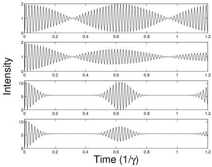
FIG. 1.: Light intensity for the number state case as a function of time $t$. Time is in units of $1/\gamma$ and light intensity is in an arbitrary units. The parameters are $g=1000\gamma$, $A=0.01g$, $B=0$ and $\delta=0$. Starting from the top: (a)$N=2$, without dissipation; (b)$N=2$, $\gamma=1$; (c)$N=11$, without dissipation; (d)$N=11$, $\gamma=1$.

The influences of the detunning and the phase-space filling are investigated in Fig. 2. For the resonant case, the light intensity will oscillate up-and-down around the center point $N/2$. However, the nonresonant coupling between the excitons and the photons will lead to the whole curve to become lower, i.e, the center line becomes more closer to the horizontal axis. Besides, the revival time becomes longer with the increase of the detunning. Comparing Fig. 2 (b) with Fig. 2 (a), we find that for the case $\delta\neq 0$, the factor $B$ will increase further the revival time. However, it is deserved to mention that if $\delta=0$, the factor $B$ does not give any feasible change to the revival time (see Eq. (28)). Our conclusion is that the revival time may be tuned by adjusting the field detuning and the phase-space filling factor .

B Coherent state case

An excitonic coherent state as the initial state was used in Ref. [5] to stimulate the linear model solutions with their experimental results and exhibited good agreement. So we continue our calculations for the coherent state case. The coherent state is characterized by $\beta=\sqrt{\langle N\rangle}\exp(i\phi)$ with the average exciton number $\langle N\rangle=\left|\beta\right|^{2}$ and the initial phase $\phi$. It should be pointed out that the definition of excitonic coherent state as the eigenstate of the annihilation operator of the excitons may work well only in the low exciton density regime [29]. This is because the expansion of a coherent state in the number state space will involve $|N\rangle_{ex}$ with large excitons number, which may destroy the weakly nonlinearity condition $NA\text{, }NB\ll g$ for the fixed $g$ and $A$. However, in the following discussions, we restrict ourself to the weakly-excitation case with smaller average exciton numbers $\langle N\rangle$ so one can still approximately describe the quantum coherence natures of the exciton systems.

The initial state of the total system $|\psi(0)\rangle=\left|\beta\right\rangle_{ex}\left|0\right\rangle_{c}$ can be written as

$$|\psi(0)\rangle=e^{-|\beta|^{2}/2}\sum_{j=0}^{\infty}\frac{\beta^{2j}}{\sqrt{(2j)!}}\left|j,j\right\rangle.$$ (29)

Substituting Eq. (29) into Eqs. (22) and (18), we get the final result for the light intensity at time $t$ in the coherent state representation

$$I_{c}(t) = \frac{\langle N\rangle}{2}\sin^{2}(2\theta)-\frac{\langle N\rangle}{2}\left\{\frac{\sin^{2}(2\theta)}{2}e^{i\Delta t}e^{-(\gamma_{1}+\gamma_{2})t/2}e^{i(A_{11}-A_{22})(\langle N\rangle-1)t}e^{-\langle N\rangle}\right.$$ (31)

$$\left.\times\exp\left[\langle N\rangle e^{-i(2A_{12}-A_{11}-A_{22})t}\left(\sin^{2}\theta+\cos^{2}\theta e^{2i(2A_{12}-A_{11}-A_{22})t}\right)\right]+c.c.\right\},$$

For the case $\delta=0$ (i.e., $\theta=\pi/4$), Eq. (31) may be reduced as

$$I_{c}(t) = \frac{\langle N\rangle}{2}\left\{1-\cos\left[(2g+B(\langle N\rangle-1))t\right]\right.$$ (33)

$$\left.\times e^{-2\langle N\rangle\sin^{2}\left(At/4\right)}e^{-(\gamma_{1}+\gamma_{2})t/2}\right\},$$

where the initial (absolute) phase of the coherent state $\phi$ does not appear in the light intensity. We find that the envelope function for the coherent state is $e^{-2\langle N\rangle\sin^{2}\left(At/4\right)}$, which may also lead to the CRs of the light intensity. However, different with the number state case, the revival time is $t=4\pi/A$, which is twice that of the number state case (comparing Fig. 3 (a) and 3 (c) with Fig. 1 (a) and Fig. 1(c)). Moreover, the phenomena of CRs with small average exciton number are more pronounced for the coherent state case than that of the number state case. In fact, the CRs can be visible even for $\langle N\rangle<1$ due to the quantum superposition properties of the excitonic coherent state. It is the same with the number state case, the results of Fig. 3(b) and Fig. 3(d) show that the decay term lowers the revival amplitude but does not modify the revival time.

The influences of the detuning and the phase-space filling for the coherent state case are also studied. Our results also confirm that the detuning will change the revival time and the revival amplitude. On the same time, the phase-space filling factor $B$ can enhance the modification of the time. However, our results show that one may remove the influence of $B$ by adjusting the detuning. In fact, for the resonant case, the conclusion of the double revival time for the coherent state case compared with that of the number state is also valid.

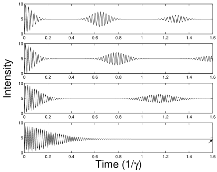
FIG. 2.: Light intensity for the number state case as a function of time $t$, obtained from Eq. (26). Time is in units of $1/\gamma$ and light intensity is in an arbitrary units. Other parameters are $g=1000\gamma$, $A=0.01g$ and $N=10$. Starting from top: (a) $\delta=0.2g$, $B=0$; (b) $\delta=0.2g$, $B=0.3A$; (c) $\delta=0.4g$, $B=0.3$; (d) $\delta=0.6g$, $B=0.3A$

To our knowledge, the CRs of Rabi oscillation in the atom-cavity system has been studied intensely, which can be described by Jaynes-Cummings model [30, 31]. When the single-mode cavity field is initially in a special state (say, coherent state), the population of the atom will exhibit CRs due to the Rabi oscillations being modulated by different mode frequencies. The CRs of the emission from the microcavity in the linear regime was studied in Ref. [32]. In their experiment, the origin of the CRs is due to quantum beat aroused from the strong coupling of the heavy-hole exciton and light-hole exciton state to the cavity photon state. Within these two systems mentioned above, linear interaction between the matter field and the light field plays a prominent role for the appearance of the CRs. The creations of CRs in nonlinear systems, such as the nonlinear directional coupler [33], the relative phase between two superfluids or superconductors [34], and the population imbalance of a two-mode Bose-Einstein condensate [35, 36, 37, 38, 25, 26] have been also studied. Here in our paper, the emission of the high-density excitons in a quantum well embedded in a single-mode cavity is also found to exhibit CRs due to nonlinear interaction between the excitons.

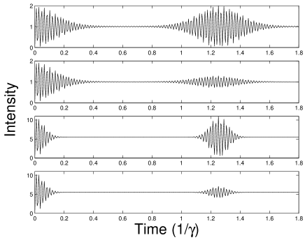
FIG. 3.: Light intensity for coherent state case as a function of time $t$. Time is in units of $1/\gamma$ and light intensity is in an arbitrary units. Other parameters are $g=1000\gamma$, $A=0.01g$, $B=0$, and $\delta=0$. From up to down: (a) $\langle N\rangle=2$, without dissipation; (b) $\langle N\rangle=2$, $\gamma=1$ (c) $\langle N\rangle=11$, without dissipation; (d) $\langle N\rangle=11$, $\gamma=1$.

IV conclusion and some remark

In summary, we have studied the emission of a semiconductor microcavity. By treating the excitons as a single-mode boson, i.e., the harmonic approximation, the analytical expressions for the light intensity are derived both for excitonic number state and coherent state. The effects of the detuning of the light field from the exciton mode, the high-order exciton-photon interaction and the dissipation are taken into account with the help of the secular approximation. The time evolution of the light emission is shown to be quite different between the number state and the coherent state cases. For the former one, the revival periods of the oscillations are $2\pi/A$. Whereas, for the excitons in a coherent state the revival periods are $4\pi/A$. The temporal decay of the exciton-polariton lowers the revival amplitude but does not modify the revival time. However, the influences of the detuning and the phase-space filling may change both the time and the amplitude. How can we exclude these complex modifications and investigate only the quantum effect of excitonic states? Our results show that, for the resonant case, the revival time is very insensitive to the changes of the factor $B$ and the time is only determined by the effective exciton-exciton interaction. We expect that our theoretical study of the phenomena of collapses and revivals would be helpful in practical experiment to measure quantum states of excitons.

Finally, we would like to emphasize that, in our theoretical treatment, the critical requirement of the CRs is the nonlinear exciton-exciton interaction but not the single-mode approximation. In fact, the treating the excitons as a single-mode harmonic oscillator is just an idealized theoretical model. For the case of a very strong coupling ($g\sim Ry_{ex}$), the effects of other exciton modes (such as $\bf{K}\neq 0$) may play important role compared with the nonlinear interactions [39, 40]. These effects will be taken into accounted elsewhere.

This work is supported by the NSF of China under Grant Nos. 10174095 and 90103024. One of the authors (GRJ) would like to express his sincerely thanks to Professor C. P. Sun and Dr. Y. X. Liu.

REFERENCES

- [1] Y. Yamamoto et al., Phys. Today 46, 66 (1993).
- [2] C. Weisbuch et al., Phys. Rev. Lett. 69, 3314 (1992); R. Houdré et al., Phys. Rev. B 49, 16761 (1994).
- [3] J. J. Hopfield, Phys. Rev. 112, 1555 (1958).
- [4] T. B. Norris et al., Phys. Rev. B 50, 14663 (1994).
- [5] J. Jacobson et al., Phys. Rev. A 51, 2542 (1995).
- [6] H. Cao et al., Appl. Phys. Lett. 66, 1107 (1995).
- [7] H. Wang et al., Phys. Rev. B 51, 14713 (1995).
- [8] S. Pau et al., Phys. Rev. B 51, 14437 (1995).
- [9] H. Wang et al., Opt. Express 1, 370 (1997).
- [10] D. Erenso et al., Phys. Rev. A 67, 013818 (2003).
- [11] E. Hanamura, J. Phys. Soc. Jpn. 29, 50 (1970); E. Hanamura and H. Haug, Phys. Rep. 33, 209 (1977).
- [12] P. G. Savvidis et al., Phys. Rev. Lett. 84, 1547 (2000).
- [13] C. Ciuti et al., Phys. Rev. B 62, R4825 (2000).
- [14] G. Messin et al., Phys. Rev. Lett. 87, 127403 (2001).
- [15] M. Saba et al., Nature 414, 731 (2001).
- [16] Y. X. Liu et al., Phys. Rev. A 61, 023802 (2000); Y. X. Liu et al., Optics Communication 165, 53 (1999).
- [17] Y. X. Liu et al., Phys. Rev. A 63, 023802 (2001).
- [18] Y. X. Liu et al., Phys. Rev. A 65, 023805 (2002).
- [19] G. R. Jin et al., (Unpublished).
- [20] Nguyen Ba An, Phys. Rev. B 48, 11732 (1993).
- [21] F. Tassone et al., Phys. Rev. B 59, 10830 (1999).
- [22] M. Kuwata-Gonokami et al., Phys. Rev. Lett. 79, 1341 (1997).
- [23] Jun-ichi Inoue et al., Phys. Rev. B 61, 2863 (2000).
- [24] G. S. Agarwal et al., Phys. Rev. A 39, 2969 (1989).
- [25] L. M. Kuang et al., Phys. Rev. A 61, 013608 (1999).
- [26] L. M. Kuang et al., Phys. Rev. A 61, 023604 (1999).
- [27] R. Houdré et al., C. R. Physique 3, 15 (2002).
- [28] T. R. Nelson et al., Appl. Phys. Lett. 69, 3031 (1996).
- [29] G. R. Jin et al., Phys. Rev. B 68, 134301 (2003).
- [30] J. H. Eberly et al., Phys. Rev. Lett. 44, 1323 (1980).
- [31] G. Rempe et al., Phys. Rev. Lett. 58, 353 (1987).
- [32] H. Cao et al., Appl. Phys. Lett. 71, 1461 (1997).
- [33] A. Chefles et al., J. Mod. Opt. 43, 709 (1996).
- [34] F. Sols, Physica B 194-196, 1389 (1994).
- [35] G. J. Milburn et al., Phys. Rev. A 55, 4318 (1997).
- [36] J. E. Williams et al., Phys. Rev. A 61, 033612 (2000).
- [37] W. D. Li et al., Phys. Rev. A 64, 015602 (2001); W. M. Liu et al., Phys. Rev. Lett. 84, 2294 (2000).
- [38] P. Zhang et al., J. Phys. B 35, 4647 (2002).
- [39] J. B. Khurgin, Solid State Commun. 117, 307 (2001).
- [40] D. S. Citrin et al., Phys. Rev. B 68, 205325 (2003).