Stabilization of Ultracold Molecules Using Optimal Control Theory

Abstract

In recent experiments on ultracold matter, molecules have been produced from ultracold atoms by photoassociation, Feshbach resonances, and three-body recombination. The created molecules are translationally cold, but vibrationally highly excited. This will eventually lead them to be lost from the trap due to collisions. We propose shaped laser pulses to transfer these highly excited molecules to their ground vibrational level. Optimal control theory is employed to find the light field that will carry out this task with minimum intensity. We present results for the sodium dimer. The final target can be reached to within 99% if the initial guess field is physically motivated. We find that the optimal fields contain the transition frequencies required by a good Franck-Condon pumping scheme. The analysis is able to identify the ranges of intensity and pulse duration which are able to achieve this task before other competing process take place. Such a scheme could produce stable ultracold molecular samples or even stable molecular Bose-Einstein condensates.

I Introduction

The creation of cold molecules from atomic Bose-Einstein condensates (BEC) DonleyNat02 ; RegalNat03 ; HerbigSci03 ; DuerrPRL04 ; XuPRL03 ; JochimSci03 ; GreinerNat03 ; ZwierleinPRL03 as well as from ultracold thermal gases NicoPRL02 ; ChinPRL03 has advanced remarkably over the last two years. In both cases molecules are formed due to interaction of atoms with an external field. The latter can be the electric field of a laser leading to photoassociation FrancoiseReview or a magnetic field tuned to drive the atoms across a Feshbach resonance Timmermans99 . Tuning close to a Feshbach resonance can furthermore be used to obtain a very large scattering length. This enhances three-body recombination and molecules are thereby formed JochimSci03 . In most experimental schemes translationally cold, but vibrationally very highly excited molecules are produced. These highly excited molecules are not stable with respect to collisions, and dimers consisting of bosonic atoms in particular are very rapidly. In the case of sodium this happens within milliseconds XuPRL03 . Creation is therefore only a first step toward novel experiments using ultracold molecules MeijerReview , and their stabilization is the obvious next task.

The ultimate goal is to create $v=0,J=0$ molecules. The task of transferring the highly excited molecules to $v=0,J=0$ is far from being trivial: a long-range molecule and a $v=0$ molecule are very different (Cf. Fig. 1 where the wavefunctions for the last bound and the ground vibrational level of the ground state of Na₂ are drawn). This task has to be solved under three major constraints: 1.) The goal has to be achieved in a time short compared to the collisional lifetime. The rate for collisional decay is not precisely known at present, but lifetimes on the order of or shorter than ms should be expected XuPRL03 . Calculations for collisional decay of molecules in highly excited vibrational levels have been performed in the non-reactive ^3,4He + H${}_{2}(v)$ case BalakrishnanPRL98 , showing an increase of the relaxation rate by nearly three orders of magnitude when the initial state is going from $v$=1 (rate $\sim$ 5$\times$ 10^-17 cm³ s^-1) to $v$=10. In the reactive Na + Na${}_{2}(v)$ case, quantum calculations for the $v=1\rightarrow 0$ rate yield $\sim 5\times 10^{-10}$cm³ s^-1 SoldanPRL02 . Therefore, at an atomic density of 10¹¹ cm^-3, a vibrational quenching relaxation time well below 1 ms is indeed to be expected. 2.) If laser pulses are to be used, spontaneous emission has to be avoided. The radiative lifetime of the excited state is on the order of 10 ns. 3.) Due to vibrational energy ”pooling” or vibration-to-vibration ladder climbing TreanorJCP67 the intermediate range of binding energies needs to be avoided at any cost, i.e. the molecules need to be immediately transferred to the lowest levels.

In this paper, we suggest to employ optimal control to transfer the highly excited molecules to the rovibrational ground state. Optimal control has been intensely studied both theoretically and experimentally in many areas of physical chemistry. Optimal control theory (OCT) RiceBook offers the prospect of driving an atomic or molecular system to an arbitrary, desired state due to the interaction with an external field. Experimentally, control is achieved via feedback learning loops, see e.g. BrixnerCPC03 for a recent review. The difference between the approach we suggest and control experiments as they have been performed over the last decade lies in the different target: In the latter the goal consists usually in varying the ratio between different dissociation channels, i.e. many final states are available and the target is rather broad, while in the present context a single ro-vibrational level is to be achieved. However, this does not pose a problem in principle – it might make control harder to achieve, but it does not render it impossible. We suggest optimal control to transfer the highly excited molecules to the rovibrational ground state because it provides an efficient method operating on a very short timescale.

Alternatively, two-photon Raman transitions have been suggested HerbigSci03 to transfer the highly excited molecules to low-lying vibrational states. However, if really the lowest vibrational levels shall be populated, a Raman scheme with continuous wave (CW) laser pulses is not conceivable due to unfavorable Franck-Condon overlaps. The framework of Stimulated Raman Adiabatic Passage (STIRAP) is not any more promising since a highly oscillatory wave function with 80% or more of its probability density in the asymptotic region can not be transferred adiabatically into a very compact wave function, typically of Gaussian shape (Cf. Fig. 1). This has been overlooked in previous studies MackiePRL00 ; DrummondPRA02 in which the vibrational degree of freedom was not explicitly taken into account.

Optimal control theory has been applied before in the context of the formation of ultracold molecules, specifically to calculate optimal conversion of an atomic into a molecular BEC HornungPRA02b . In this work, a laser pulse was employed together with a magnetic field which induced a Feshbach resonance. The authors worked in the framework of the Gross-Pitaevski equation which is a non-linear Schrödinger equation while employing a linear variant of OCT. A nonlinear version of OCT as required for the application to the Gross-Pitaevski equation has been worked out recently SklarzPRA02 . The vibrational structure of the molecules was simply taken into account by assigning a few vibrational levels in Ref. HornungPRA02b , but the coordinate-dependence of the vibrational wave functions, in particular the qualitatively different character of initial and final state wave functions, was neglected. Finally, the initial state in Ref. HornungPRA02b corresponds to two free, colliding atoms. If one was to include the vibrational structure in the model of Ref. HornungPRA02b , the resulting Hilbert space would be infinite-dimensional, and due to the theorem of controllability RamakrishnaPRA95 ; TarnClark one would not be guaranteed that an optimal solution exists at all.

For conceptual clarity, we will therefore separate the creation of molecules, however weakly bound, from the process of their stabilization. This approach corresponds furthermore nicely to the current status of experiments on cold molecules which create weakly bound dimers via magnetic Feshbach resonances or three-body recombination RegalNat03 ; HerbigSci03 ; DuerrPRL04 ; XuPRL03 ; JochimSci03 ; GreinerNat03 ; ZwierleinPRL03 . The stabilization of these molecules in the experiment still remains an open problem to which no easy answers exist. In this paper, we will hence start from extremely weakly bound molecules and employ optimal control theory to obtain short, shaped laser pulses which drive the system from a specified, highly excited vibrational level to the ground state.

We will apply the optimal control algorithm to the formation of stable sodium dimers. From molecular spectroscopy experiments with CW lasers ElbsPRA99 , we know that a pathway connecting the rovibrational ground state with the last bound levels exists. Furthermore, sodium has been one of the first systems to be studied by femtosecond spectroscopy BaumertPRL90 and control experiments ShnitmanPRL96 . Its properties under ultracold conditions are equally well studied, see e.g. McKenziePRL02 ; XuPRL03 . The scheme we suggest is similar in spirit to that of Ref. VardiJCP97 where nanosecond pulses were used. In order to compare to current experimental control techniques, however, we employ pulses of femtosecond and picosecond timescale. These pulses are optimized by the control algorithm while they would serve as input for a feedback learning loop in a prospective experiment, see e. g. BrixnerCPC03 . This is in contrast to the intuitively chosen pulses of Ref. VardiJCP97 . A large number of theoretical studies on femtosecond pulse control of sodium has been reported, mostly in the context of photodissociation and ionization, see e.g. MachholmJCP96 ; PaciJCP98 ; ShenCPL03 . Our approach has been motivated by the experiment of Ref. ElbsPRA99 where the last bound levels of the Na₂ ground state were probed. This was achieved by exciting $v=0$ Na₂ molecules from a molecular beam with CW lasers to an excited electronic state and subsequent spontaneous emission. A scheme with multiple excitation-deexcitation steps was necessary due to Franck-Condon overlaps. In principle, one could invert this scheme to create $v=0$ from highly excited molecules. However, the yield would be low and the required times cannot compete with the time scales of collisional loss and spontaneous emission. We therefore look for optimal ultrashort pulses which realize this inverse scheme.

We formulate the problem as one of optimizing state-to-state transitions. This is in contrast to a density matrix formulation which describes transitions from an ensemble of states to another one AllonJCP93 ; JosePRL02 . As an extreme case, the latter includes true cooling as a transition from an ensemble of states to a single state. Note, that true cooling requires coupling to a dissipative environment which accepts the entropy AllonJCP97 ; AllonCP01 . However, the optimization of state-to-state transitions should be sufficient for Bose-condensed samples since one starts with a coherent sample. Even in the case of thermal samples state-to-state transitions can serve as an important first step in which one state is selected to be transferred while all others are ionized. We will employ OCT in the Krotov variant restricting the change in pulse energy at each iteration SklarzPRA02 ; AllonCP01 ; JosePRA03 . This guarantees monotonous and smooth convergence toward the objective.

We will work in the framework of the linear Schrödinger equation which describes the internuclear dynamics of two atoms, i.e. in case of a Bose-Einstein condensate (BEC) we neglect the condensate dynamics. This approach is justified by the time scales present in standard optical and/or magnetic traps. While the internuclear dynamics and pulse shaping occur on the time scale of femtoseconds to picoseconds, the condensate dynamics for conventional traps is characterized by microseconds. The condensate will have to adjust to the new internal state, but this is going to happen on a much slower time scale than the one of the pulse PascalPRA03 . We can hence safely ignore the influence of the condensate on the dynamics of the state-to-state transition and assume that the adjustment of the condensate takes place once the pulse is over.

The paper is organized as follows: The model for the sodium dimer as well as the proposed scheme to form stable ultracold molecules are described in Section II. Section III briefly reviews the optimal control algorithm with details given in the Appendix. The results are presented in Section IV. Section V concludes with a discussion of the experimental feasibility of our proposed scheme as well as its implications to vibrational cooling.

II The Na₂ system

We have chosen Na₂ because this system has been intensely studied in ultracold experiments, in control experiments, and by traditional spectroscopy, and a large amount of experimental data is available. In particular, highly accurate potential energy curves have been obtained from molecular spectroscopy SamuelisPRA00 ; TiemannZfPD96 . Experiments ElbsPRA99 have furthermore shown that a route from the last bound levels to $v=0$ exists. In this scheme, ground state molecules from a molecular beam with $v=0$, $J=0$ are excited by a CW laser ($\lambda=610$ nm) to the A${}^{1}\Sigma^{+}_{u}$ excited state ($v^{\prime}=15$). Those molecules which decay to the $v=29$ level of the ground state, are excited by a second CW laser ($\lambda=540$ nm) to excited state levels with $v^{\prime}=100-140$. A third CW laser ($\lambda=595$ nm) probes the transition between these excited state levels and the last bound levels ($v=61-65$) of the ground state.

II.1 Proposed scheme for the formation of ultracold, stable molecules

We envisage the following two-step scheme for the production of ultracold molecules (Fig. 1).

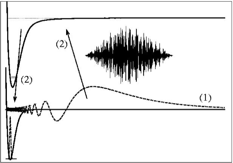
Figure 1: Scheme for the production of stable ultracold molecules: Vibrationally highly excited molecules are created due to the interaction with an external field (1) and are transferred to the ground state by a shaped laser pulse (2). The wave functions of the last bound and the $v=0$ levels are drawn as dashed lines, while the excited state vibrational levels which have good Franck-Condon overlap with the last level and with the ground level, respectively, are indicated by dotted lines. Obviously, no direct transition exists.

First, loosely bound molecules are created by tuning an external magnetic field to sweep an atomic sample across a Feshbach resonance RegalNat03 ; HerbigSci03 ; DuerrPRL04 ; XuPRL03 or by enhanced three-body recombination in the vicinity of a Feshbach resonance JochimSci03 . Another possibility is given by applying a weak off-resonant CW photoassociation laser. The last level is so extremely loosely bound that even a very weak field perturbs it leading to a coupling with the continuum states Philpel . Second, a shaped laser pulse is applied to transfer the highly excited molecules to $v=0$. This second step is of our concern in the present study. Following the experiment ElbsPRA99 , we propose to employ fields which induce transitions between the Na₂ ground state ($X^{1}\Sigma^{+}_{g}$ ) and the A${}^{1}\Sigma^{+}_{u}$ excited state.

One could imagine a one-step scheme where the optimal pulse is used to directly transfer a continuum wave function to the ro-vibrational ground state. However, in the case of continuum states the theorem of controllability RamakrishnaPRA95 ; TarnClark is not applicable and one is not guaranteed that an optimal solution exists. Furthermore, the results may depend on how the continuum is modelled. Since experimentally, step (1) seems to become a standard technique RegalNat03 ; HerbigSci03 ; DuerrPRL04 ; XuPRL03 , we prefer to restrict the task of the optimal pulse to the transfer of one bound level to another bound level and to attain a mathematically well-defined model.

II.2 Model and methods

We are interested in obtaining an estimate of the feasibility of optimal control experiments with ultracold molecules. We therefore restrict our approach to a qualitative model with two channels which correspond to the two electronic states of Ref. ElbsPRA99 , and we neglect hyperfine interaction, spin-orbit coupling and rotational excitation. These effects should be included to make quantitative predictions.

Taking hyperfine interaction into account would amount to studying a model with more than two channels. At the binding energies at which cold molecules are created in the current experiments, a single channel description for the ground state is not valid SamuelisPRA00 , i.e. the wave function contains singlet as well as triplet components. The shaped laser pulse does not alter the coherence of this superposition. A multi-channel treatment would therefore result in a pulse with parts corresponding to the excitation pathway of singlet, and other parts corresponding to the excitation pathway of triplet molecules. However, in this study we want to emphasize the importance of the internal structure of the molecules, i.e. the coordinate-dependence of the atom-atom interaction potentials, for the creation of stable molecules. We therefore restrict the model to two channels, one for the ground and one for the electronically excited state, and we perform calculations for singlet states. This amounts to neglecting the triplet component of the wave function. If the triplet component of the wave function is larger than the singlet component, one would have to repeat the present calculations using the corresponding triplet potentials. The qualitative principle, however, remains unaltered.

The argument concerning rotational excitation is along the same lines as in the case of hyperfine interaction. Allowing for rotational excitation would amount to treating additional channels with the centrifugal barrier for each $J$ added to the atom-atom interaction. The additional channels increase the size of the search space, but at the same time allow for more pathways, i.e. for more flexibility. It is thus not clear a priori whether the search for optimal pulses will be slowed down or sped up. Moreover, if the initial state contains some rotational excitation, one might speculate that this facilitates control since such a wave function would be more bound than one with $J=0$. Of course, such a claim can only be proven by a detailed investigation which is beyond the scope of the present work.

We solve the radial Schrödinger equation for the vibrational motion of the sodium dimer,

$$i\hbar\,\frac{\partial}{\partial t}\,\varphi(R,t)=\boldsymbol{\mathsf{\hat{H}}}\,\varphi(R,t)\,,$$ (1)

with $R$ the distance between the two nuclei. The vibrational wave function consists of two components, $\varphi=\begin{pmatrix}\varphi_{g}\\ \varphi_{e}\end{pmatrix}$, corresponding to the two channels. The Hamiltonian describing two electronic states and the nuclear degree of freedom, $R$, is given by

$$\boldsymbol{\mathsf{\hat{H}}}=\begin{pmatrix}\boldsymbol{\mathsf{\hat{T}}}+\boldsymbol{\mathsf{\hat{V}}}_{g}&0\\ 0&\boldsymbol{\mathsf{\hat{T}}}+\boldsymbol{\mathsf{\hat{V}}}_{e}\end{pmatrix}+\begin{pmatrix}0&\boldsymbol{\mathsf{\hat{\mu}}}\,\varepsilon(t)\\ \boldsymbol{\mathsf{\hat{\mu}}}\,\varepsilon(t)^{*}&0\end{pmatrix}\,,$$ (2)

where $\boldsymbol{\mathsf{\hat{T}}}=\frac{\hbar}{2m}\frac{\partial}{\partial R}$ denotes the kinetic energy operator, $\boldsymbol{\mathsf{\hat{\mu}}}$ the dipole operator and $\varepsilon(t)$ the electric field. The ground state potential $\boldsymbol{\mathsf{\hat{V}}}_{g}$ describes the state of $X^{1}\Sigma_{g}$ symmetry which is correlated to the (3s+3s) asymptote of sodium, and the excited state potential $\boldsymbol{\mathsf{\hat{V}}}_{e}$ describes the state of $A^{1}\Sigma_{u}$ symmetry correlated to the (3s+3p) asymptote. The ground state potential has been obtained by an analytical fit to high-resolution spectroscopic data SamuelisPRA00 , while an RKR potential TiemannZfPD96 has been matched to an asymptotic expansion MarinescuPRA95 for the excited state potential. We assume the dipole operator to be independent of $R$, $\boldsymbol{\mathsf{\hat{\mu}}}=\,$const. While this approximation needs to be improved, it might well serve as a first step since the two concerned electronic states do not show avoided crossings. The electric field is taken to be real which means that a fixed (but not specified) polarization is assumed. The initial guess field is given by $\varepsilon(t)=\varepsilon_{0}\,S(t)\cos(wt)$ where $S(t)$ is a Gaussian envelope function or a sequence of Gaussians and $\omega$ is the central frequency of the pulse.

The wave function $\varphi(R,t)$ is represented on a grid employing the mapped Fourier grid method SlavaJCP99 which allows for accurately representing even the last bound levels of the ground state potential with a comparatively small number of grid points ($N=1024$). The mapped Fourier grid method introduces, however, unphysical states which can lead to spurious effects in the dynamics. For the sodium system, these ”ghost” states can be eliminated by using a basis of sine functions (instead of plane waves) WillnerJCP04 and by choosing the density of points sufficiently high. The mapped grid is calculated from the envelope potential of both $\boldsymbol{\mathsf{\hat{V}}}_{g}$ and $\boldsymbol{\mathsf{\hat{V}}}_{e}$, i.e. the same grid is used on both channels.

The time-dependent Schrödinger equation, Eq. (1), is solved formally by

$$\varphi(R,t)=\boldsymbol{\mathsf{\hat{U}}}(t,0)\,\varphi(R,0)\,.$$ (3)

We employ a Chebychev expansion RonnieReview94 ; RonnieGrid96 of the time evolution operator, $\boldsymbol{\mathsf{\hat{U}}}(t)$, which is numerically exact for a time-independent Hamiltonian. In our case of an explicitly time-dependent Hamiltonian, Eq. (3) is second order in the time step. Note, that we cannot use a less expensive propagation method such as the split propagator since the grid mapping introduces multiplications between functions in Fourier space and functions in real space, i.e. terms of the kind $f(R)\frac{\partial}{\partial R}$.

The initial state as well as the target state are taken to be eigenstates of the ground state potential. The eigenstates are computed simply by calculating a matrix representation of the Hamiltonian in the sine basis and subsequent diagonalization WillnerJCP04 .

III The Optimal Control Algorithm

We formulate the optimal control for state-to-state transitions, i.e. we want to find the field which drives a specified initial state $|\varphi_{i}\rangle$ to a specified target state $|\varphi_{f}\rangle$ at the final time $t=T$. The objective we want to reach can therefore be defined as the overlap between the initial state propagated from time $t=0$ to $t=T$ with field $\varepsilon(t)$ and the target state,

$$F=|\langle\varphi_{i}|\boldsymbol{\mathsf{\hat{U}}}^{+}(T,0;\varepsilon)|\varphi_{f}\rangle|^{2}\,.$$ (4)

$\boldsymbol{\mathsf{\hat{U}}}^{+}(T,0;\varepsilon)$ denotes the evolution operator which completely specifies the system dynamics. In the calculations presented below, $|\varphi_{i}\rangle$ will be a highly excited vibrational level of the Na₂ ground state, while $|\varphi_{f}\rangle$ will be chosen to be the vibrational ground state of the Na₂ ground state. The length of the optimization time interval, $T$, is an external parameter of the calculation. If one compares to experiment, it is related to the bandwidth of the pulse and the number of pixels of the pulse shaper. Taking $T$ to be twice the longest vibrational period which occurs in the problem is usually a good guess. In the case of long-range molecules, very different time scales are involved which leads to a problem of feasibility. We present a work-around in Sec. IV.3. A field is optimal if it almost completely transfers the initial state $|\varphi_{i}\rangle$ to the target $|\varphi_{f}\rangle$, i.e. if $F$ attains a value close to one.

The objective $F$ is a functional of the field $\varepsilon(t)$. However, it depends explicitly only on the final time $T$. To use information from the dynamics at intermediate times, i.e. within the time interval $(0,T)$, we define a new functional $J$,

$$J=-F+\int_{0}^{T}g(\varepsilon,\varphi)\mathrm{d}t\,,$$ (5)

where the integral term denotes additional constraints over the system evolution. The optimal field will be found by minimization of $J$. The additional constraints provide the connection between the dynamics and reaching the objective, they therefore define how the control is accomplished SklarzPRA02 . This becomes particularly apparent in the Krotov variant of optimal control theory (see SklarzPRA02 for a review) which we will employ in the following. The Krotov method allows us to derive an iterative procedure which maximizes the original functional $F$ (minimizes $-F$) at the final time $T$ while modifying the field at intermediate times and guaranteeing monotonic convergence. Details can be found in Appendix A.

The choice of $g(\varepsilon,\varphi)$ is not arbitrary, it needs to comply with the requirement of monotonic convergence JosePRA03 (see also Appendix A). In this study, we use

$$g(\varepsilon,\varphi)=g(\varepsilon)=\frac{\alpha}{S(t)}\left[\varepsilon(t)-\tilde{\varepsilon}(t)\right]^{2}\,,$$ (6)

where $\tilde{\varepsilon}(t)$ is the field of the previous iteration. $S(t)$ denotes the constraint to smoothly switch the field on and off with shape function $S(t)$. We take it to be Gaussian or $S(t)=\sin^{2}(\pi t/T)$. Eq.(6) has the physical interpretation of restricting the change in pulse energy at each iteration. It allows for a smooth convergence toward the objective since the change in field vanishes when the optimal field is approached JosePRA03 . The optimization strategy can be controlled by the parameter $\alpha$: A small value results in a small weight of the additional constraint and allows for large modifications in the field, while a large value of $\alpha$ represents a conservative search strategy allowing only small modifications of the field at each iteration. The parameter $\alpha$ is not directly related to the number of iterations required to find a solution, and the best search strategy is usually given by running the optimal control algorithm first with a small and then with a large value of $\alpha$ HornungPRA02a : A small $\alpha$ will excite many pathways, then the solution can be refined with large $\alpha$.

With this choice of $g(\varepsilon,\varphi)$ the change in field, $\Delta\varepsilon=\varepsilon^{\mathrm{new}}-\varepsilon^{\mathrm{old}}$, at every time $t$, $0<t<T$, is given by

$$\Delta\varepsilon(t) = \frac{S(t)}{\alpha}\;\mathfrak{Im}\left[\;\langle\underbrace{\varphi_{i}|\,\boldsymbol{\mathsf{\hat{U}}}^{+}(T,0;\varepsilon^{\mathrm{old}})}\,|\varphi_{f}\rangle\;\langle\underbrace{\varphi_{f}|\,\boldsymbol{\mathsf{\hat{U}}}^{+}(t,T;\varepsilon^{\mathrm{old}})}\,\boldsymbol{\mathsf{\hat{\mu}}}\,\underbrace{\boldsymbol{\mathsf{\hat{U}}}(t,0;\varepsilon^{\mathrm{new}})\,|\varphi_{i}\rangle}\;\right]$$

$$\quad\quad\quad\quad\quad\quad\quad\mathrm{forward}\quad\quad\quad\quad\quad\mathrm{backward}\quad\quad\quad\quad\mathrm{forward}$$

(see Appendix A for the derivation). The change in field is determined by the ”expectation value” of the dipole operator $\boldsymbol{\mathsf{\hat{\mu}}}$, i.e. by matching at time $t$ the initial wave function which has been propagated forward in time from $t=0$ to $t$ with the target wave function which has been propagated backward in time from $T$ to $t$. Note, that this is not an ordinary quantum mechanical expectation value due to the different fields, $\varepsilon^{\mathrm{old}}$ of the previous iteration and $\varepsilon^{\mathrm{new}}$ of the current iteration. We consider two channels/electronic states for the Na₂ system. The wave function therefore contains two components, $\begin{pmatrix}\varphi_{g}\\ \varphi_{e}\end{pmatrix}$, and the dipole operator, $\begin{pmatrix}0&\boldsymbol{\mathsf{\hat{\mu}}}\\ \boldsymbol{\mathsf{\hat{\mu}}}&0\end{pmatrix}$, induces electronic transitions. Note that while for the initial and target state $\varphi_{e}=0$, the propagated states have a non-zero $\varphi_{e}$-component due to the field.

Eq. (III) implies that information from the dynamics in both the past and the future is used to calculate the new field. The iterative algorithm is thus defined: We first pick a guess field $\varepsilon^{\mathrm{old}}$, propagate $|\varphi_{i}\rangle$ with $\boldsymbol{\mathsf{\hat{U}}}(T,0;\varepsilon^{\mathrm{old}})$ (forward) and evaluate the objective. We then propagate the target state $|\varphi_{f}\rangle$ from time $t=T$ to time $t=0$ (backward), storing the propagated wave function for all intermediate times. In a third step we obtain the new field $\varepsilon^{\mathrm{new}}$ at each time $t$ by evaluating Eq. (III) and we use $\varepsilon^{\mathrm{new}}$ to propagate $|\varphi_{i}\rangle$ (forward). These steps have to be repeated until the objective has reached the desired value close to one.

Note that since $\Delta\varepsilon=\varepsilon^{\mathrm{new}}-\varepsilon^{\mathrm{old}}$, Eq. (III) is implicit in the new field $\varepsilon^{\mathrm{new}}$. A simple, but sufficient remedy to avoid solving this implicit equation is found by employing two different grids in the time discretization JosePRA03 . The time grid for the wave functions has $N_{t}+1$ points and is defined from $t=0$ to $t=T$, while the grid where the field is evaluated has $N_{t}$ points and ranges from $t=\Delta t/2$ to $t=T-\Delta t/2$ with $\Delta t=T/N_{t}$ the spacing for both grids. The new field $\varepsilon^{\mathrm{new}}$ at the first interleaved grid point $t=\Delta t/2$ is then calculated from the wave function at $t=0$, i.e. from $\boldsymbol{\mathsf{\hat{U}}}(0,0;\varepsilon^{\mathrm{new}})\,|\varphi_{i}\rangle=|\varphi_{i}\rangle$, while the wave function is propagated from $t=0$ to $t=\Delta t$ using the field $\varepsilon^{\mathrm{new}}(\Delta t/2)$. This process is repeated for all other time grid points.

IV Results and discussion

In the proposed scheme, the ultracold molecules are formed in one of the last bound levels, close to the dissociation limit. We have investigated states from the whole range of the vibrational spectrum ($v=10$, $v=40$, $v=62$) in order to gain a deeper understanding of the physical mechanism behind the control. Recall that the last bound level of the ground state of the sodium dimer has quantum number $v=65$.

Optimal pulses transferring all initial states to the target state ($v=0$) were found if the guess pulse was chosen in a physically sensible way. This means that the pulse spectrum should coincide with the transition frequencies between vibrational levels in the ground and excited state which have a good Franck-Condon overlap. The transition frequencies with non-negligible Franck-Condon overlap range from about 6000 cm^-1 to about 13000 cm^-1. This corresponds to a transform limited pulse of 5 fs full width half maximum (FWHM). However, not the whole spectral range of 7000 cm^-1 needs to be covered. The Franck-Condon overlaps of the initial and the target state with the vibrational levels of the excited state indicate one or two spectral regions which should be important in the transfer. It was sufficient to accordingly choose one or two central frequencies of the guess pulse. Convergence to reach 99% of the objective could then be achieved with a relatively small number of iterations.

IV.1 Simple search strategies

In addition to the spectral range covered by the pulse (cf. Fig. 2), the rate of convergence depends on the two control knobs of the optimal control algorithm, the intensity of the pulse or the integrated pulse energy and the length $T$ of the optimization time interval. If we choose a comparatively high intensity and long time $T$ ($T\geq T^{*}=2\pi/\omega=2\pi h/|E_{v}-E_{v-1}|$ with $E_{v}$ the binding energy of level $v$), we allow the algorithm a lot of freedom. Convergence to 99% of the objective is then reached very fast ($N_{\mathrm{it}}\leq 30$). This corresponds to a few hours of CPU time for $v=10$ and $v=40$ and to a few days for $v=62$ on a Linux PC (the increase for $v=62$ is caused by the necessity to store the backward propagated wave functions on disc rather than in memory for long time intervals).

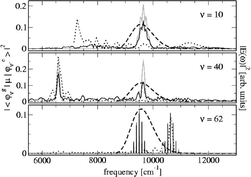
Figure 2: The Franck-Condon overlaps of the intial state ($v=10,40,62$, dotted lines) and of the target state ($v=0$, dashed lines) with all excited state vibrational levels ($v^{\prime}$) are shown vs. frequency. Also shown are the spectra of obtained optimal fields (solid black lines) and of the corresponding guess fields (solid grey lines).

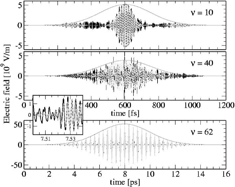
Figure 3: The optimal fields (black solid lines) corresponding to Fig. 2. Also plotted are the respective guess fields (dashed lightgrey lines) and the shape function $S(t)$ (solid darkgrey lines). The differences between optimal and guess fields for $v=62$ can hardly be seen on the time scale of 16 ps, therefore the inset shows the enlargement of a small interval.

The resulting pulses are shown in Figs. 2 and 3. A sequence of pulses with 100 fs FWHM was chosen for $v=10$ and $v=62$, while a single pulse of 355 fs FHWM was taken as guess for $v=40$. The spectra of the pulses (solid lines in Fig. 2) are compared to the Franck-Condon overlaps of the initial (dotted lines) and target (dashed lines) state with all vibrational levels of the excited state potential. For the target state $v=0$, the Franck-Condon overlaps with all excited state vibrational levels are characterized by a simple broad peak between 8700 cm^-1 and 11000 cm^-1. The corresponding vibrational levels of the excited state have quantum numbers $v^{\prime}=1$ to $v^{\prime}=20$.

For initial state $v=10$, non-zero Franck-Condon overlaps can be found between 7150 cm^-1 and 12500 cm^-1 corresponding to levels $v^{\prime}=0$ to $v^{\prime}=54$. In this case, the control task is comparatively simple: There is a number of excited state vibrational levels which have good Franck-Condon overlap with both the initial and the target state, i.e. a direct pathway exists. The simplest solution is therefore given by a pulse which addresses the transition frequencies between these ”common” levels ($v^{\prime}=1$ to $v^{\prime}=20$) and initial and target state. This solution is rapidly found by the optimal control algorithm: The transition frequencies between these ”common” levels ($v^{\prime}=1$ to $v^{\prime}=20$) and the target state are already contained in the guess pulse (grey line in Fig. 2), and the transition frequencies between the ”common” levels and the initial state around 7800 cm^-1 can clearly be seen in the spectrum of the optimal pulse. Since the guess pulse is rather intense, other pathways are excited as well. If an initial guess which is even closer to the direct pathway solution, i.e. a pulse with two central frequencies is employed, optimal solutions can be found with less intensity and larger FHWM, i.e. smaller spectral bandwidth (not shown). Note, that even in this simple case where the solution basically can be guessed, the knowledge of only the transition frequencies is not enough. Such a guess pulse with two central frequencies transfers less than 1% from the initial to the target state while the time-frequency correlations of the optimal pulse allow for more than 99% transfer.

The situation becomes more involved for higher excited initial states. No direct pathways, i.e. no excited state vibrational levels which simultaneously have good Franck-Condon overlap with initial and target state exist. Moreover, non-zero Franck-Condon overlaps with the excited state vibrational levels are usually found in different spectral regions for the initial and the target state. The guess pulses are therefore chosen to contain two central frequencies addressing the relevant transition frequencies. If sufficient intensity is allowed, a solution can rapidly be found. The intensity is needed to find other pathways which are not contained in the guess pulse, and the resulting spectrum is rather broad (cf. Fig. 2, middle panel). Note furthermore the different time scales in Fig. 3 where the length of the time interval $T$ has been chosen to be at least twice the vibrational period of the initial state. Since the level $v=62$ is very close to the dissociation limit, its binding energy is very small and its vibrational period is very long. The required $T$ increases up to 240 ps for $v=65$. Such long times obviously pose a problem, this will be addressed in Sec. IV.3.

IV.2 Restricting the pulse intensity

Since optimal control is based on constructive and destructive interference between different quantum pathways, the intensity of the pulse must be sufficiently high to excite several such pathways. Furthermore the guess pulse must contain sufficient intensity in the relevant modes for the algorithm to find a solution. If the overlap of the initial state propagated with the guess field and the target state is very small in Eq. (III), the changes in the field are also very small. The algorithm then needs a very large number of iterations, or it may not converge at all. Therefore there exists a minimum intensity necessary to find a solution. Note that the minimum intensity we have found theoretically does not necessarily have to be the same in a corresponding experiment. This is due to the differents ways in which a solution is obtained theoretically and experimentally. The relation between the two still needs to be clarified which is, however, beyond the scope of the present work.

The integrated pulse energy is given by

$$\mathcal{E}_{P}=\epsilon_{0}\,c\,A\,\int_{0}^{\infty}|E(t)|^{2}\,\mathsf{d}t$$ (8)

with $E(t)$ the optimal field, $A$ the area which is covered by the laser ($A=\pi r^{2}$ with $r=300\mu$m), $c$ the speed of light and $\epsilon_{0}$ the electric constant. The integration can be done numerically over the optimal field or analytically over the shape function, the latter usually being sufficient to obtain an estimate.

$v$ (initial state)	10	40	62
$\mathcal{E}_{\mathrm{pulse}}$	60 $\mu$J	1.5 mJ	3.9 mJ

Table 1: Minimum intensities needed to find a convergent solution transferring the initial state ($v=10,40,62$) to the ground state ($v=0$)

Table 1 lists the minimum pulse energy necessary to find an optimal solution within $N_{it}\leq 100$ iterations for $v=10$, $v=42$, and $v=62$. The increasing difficulty of the control task with increasing vibrational excitation is reflected in the increase in required pulse energy.

Since part of the intensity is necessary to find the relevant frequencies, one can speculate that it should be possible to further reduce the intensity by dividing an optimal field which contains already the relevant frequencies by some factor and to restart the optimal control algorithm. This is indeed possible. New optimal solutions within a reasonable number of iterations were found after dividing the optimal field of a previous calculation by a factor between two and five (reducing the pulse energy by a factor between four and 25). Using an analytical guess with the corresponding intensity did not lead to a convergent solution. An example is shown for $v=62$ in Fig. 4.

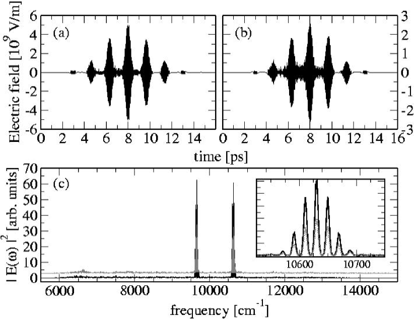
Figure 4: The fields (a-b) and spectra (c) of optimal fields for $v=62$. The spectrum of the stronger pulse (a) is plotted in black while the spectrum of weaker field (b), slightly shifted for visibility, is plotted in grey. The inset shows an enlargement of the high-frequency peak.

The spectrum of the weaker field becomes broader, in particular new peaks appear at about 6600 cm^-1 and 7800 cm^-1. The dynamics induced by the two optimal fields of Fig. 4 has been analysed by calculating the time-dependent population of vibrational levels, $|\langle\varphi_{v/v^{\prime}}|\varphi_{g/e}(t)\rangle|^{2}$. The number of levels which attain at some time $t$ a population of more than 10% and 5%, respectively, are given in Table 2.

	$E_{0}=0.01$ a.u.	$E_{0}=0.005$ a.u.
	$\mathcal{E}_{\mathrm{pulse}}=16$ mJ	$\mathcal{E}_{\mathrm{pulse}}=4$ mJ
$N^{\mathrm{ground}}_{\mathrm{Pop>0.10}}$	3	6
$N^{\mathrm{ground}}_{\mathrm{Pop>0.05}}$	23	13
$N^{\mathrm{excited}}_{\mathrm{Pop>0.10}}$	7	7
$N^{\mathrm{excited}}_{\mathrm{Pop>0.05}}$	24	16

Table 2: Number of vibrational levels of ground and excited state whose population exceeds 10% ($N_{\mathrm{Pop>0.10}}$) and 5% ($N_{\mathrm{Pop>0.05}}$) at some time $t$ ($0<t<T$). Note that the 7 excited state levels with more than 10% population are not the same for 16 mJ and for 4 mJ.

The weaker pulse populates a smaller number of vibrational levels. It is interesting to note that the levels which get populated are not the same for the weaker and the stronger pulse. Hence, a different solution is found after the reduction of intensity. This is confirmed by the objective $F$ being $F=7.9\cdot 10^{-5}$ after the division of the optimal field by a factor of two, but becoming $F=0.97$ after 25 more iterations of the algorithm. The fact that the field is not simply scaled but a new solution needs to be found, explains why the intensity of the field can only be reduced by a factor between two and five, but not by one or two orders of magnitude. Again, while some information is already contained in the field, a certain minimum intensity is needed to excite other pathways which constitute the new solution.

IV.3 Restricting the optimization time $T$

The optimization time $T$ is a parameter of the calculations, and as explained in Sec. IV.1 a good guess is given by taking $T$ to be twice the time corresponding to the smallest frequency which occurs in the problem. Since we are interested in the last bound levels, this time becomes very large (on the order of nanoseconds for Na₂). Such a time scale is too long to efficiently compete with collisions and spontaneous emission.

Simply choosing a smaller value of $T$ does not solve the problem. In this case, the optimal control algorithm did not find any solution for many different guess pulses. A comparatively simple remedy to the problem was found by using the result of an optimization with a large value of $T$, restricting it in time, and employing this modified field as initial guess pulse for a second run of the optimization algorithm. The restriction in time was done by Fourier-transforming the field, deleting points in frequency space and Fourier-transforming it back to the time domain. Keeping only every 10th value of the field in frequency space reduces the time interval by a factor of 10. The shape function for the second optimization run was chosen to be $S(t)=\sin(\pi t/\tilde{T})$ where $\tilde{T}$ denotes the reduced time interval.

Such a reduction of the optimization time has been tested for up to a factor of 20. Remarkably, it did not matter whether the points in frequency space were deleted symmetrically around $\omega=0$ or not. There is no rigorous upper limit to the factor, by which $T$ can be reduced. However, the more $T$ is reduced, the slower becomes the convergence. There is furthermore no upper limit to the objective which can be reached with reduced $T$. This is shown in Fig. 5 where the objective is plotted vs. the number of iterations of the control algorithm.

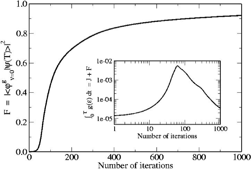
Figure 5: Convergence of the optimal control algorithm after the total time $T$ (corresponding to the vibrational period of the initial state) has been reduced by a factor of 8.

After reducing $T$ by a factor of 8, a field which transfers more than 90% of the initial state to $v=0$ is found after $N_{\mathrm{it}}\sim 1000$ iterations. Note, that each iteration requires a full time propagtion. Nevertheless, the calculations do not become prohibitively expensive due to the shorter propagation time ($T/8$). The inset of Fig. 5 shows $\int_{0}^{T}g(\varepsilon)\,\mathsf{d}t$ vs. the number of iterations. The integral corresponds to the value by which the objective is increased at each iteration, While this value decreases algebraically after about 60 iterations, it is still sufficient to increase the objective from about 20% after $N_{\mathrm{it}}=60$ to more than 90% after $N_{\mathrm{it}}=1000$. The larger number of required iterations is not only due to the restriction in time, but also due to a reduction in integrated pulse energy and hence intensity.

An example of an optimal field and its spectrum after $N_{\mathrm{it}}=1000$ are shown in Fig. 6.

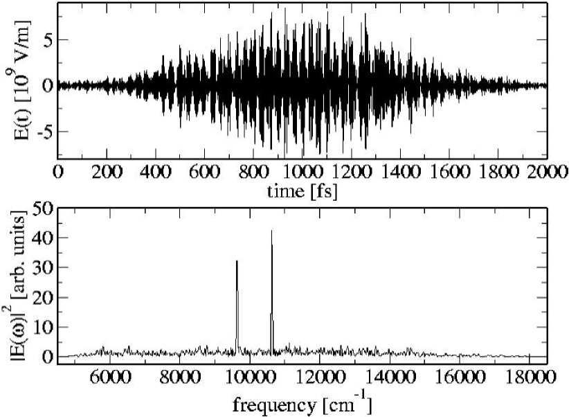
Figure 6: The optimal field and its spectrum. The optimization time interval has been reduced by a factor of 8.

The field shows a sequence of very short sub-pulses which is characteristic for optimal fields HornungPRA02a . The spectrum is rather broad, covering about 9000 cm^-1. It should be noted, however, that already the spectrum after the first optimization run with large $T$ was rather broad. At this point it is very difficult to decide whether this broadness is physically necessary or or whether it is an arteficial by-product of the mathematical algorithm. Unfortunately, it is not possible in a straightforward way to include a restriction in bandwidth as condition in the algorithm without ruining the property of monotonous convergence (see App. B for a more detailed discussion).

More insight is gained by analyzing which vibrational levels the optimal field populates during the course of time. Fig. 7 shows the total population of the two channels (solid black lines) with the optimal field (in grey) which has been scaled for comparison.

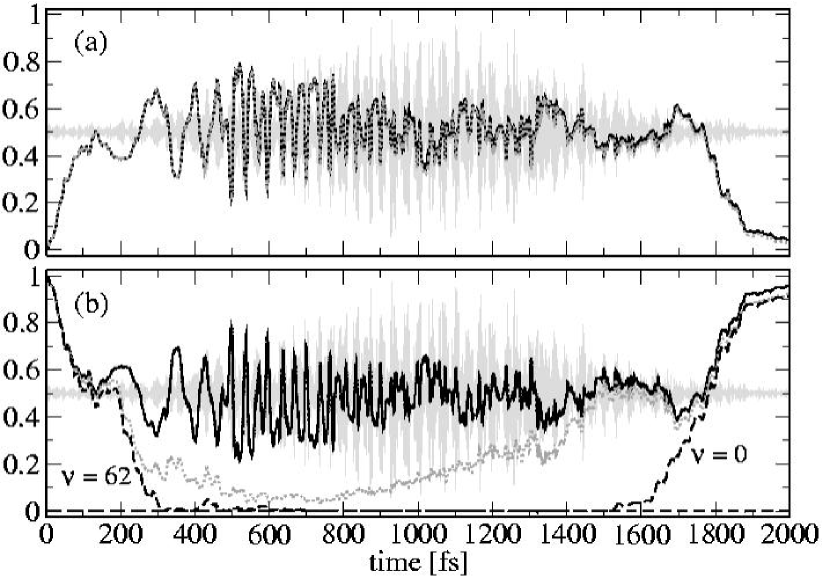
Figure 7: Population analysis of the dynamics with the optimal field for the electronically excited state (a) and the ground state (b). The total population $\big{|}\langle g/e|\Psi(t)\rangle\big{|}^{2}$ (solid black line) is compared to the sum of populations of all bound vibrational levels $\sum_{v}|\langle\varphi^{g/e}_{v}|\Psi(t)\rangle|^{2}$ (dotted grey line) with the field plotted in the background (lightgrey, scaled for comparison). For the excited state, the black and the grey line are almost identical indicating that the continuum is not populated, while the curves differ for the ground state indicating significant population of the continuum at intermediate times. Panel (b) shows furthermore the population of initial ($v=62$) and target ($v=0$) vibrational level (dashed lines).

The sub-pulse structure of the field corresponds to population cycling between ground and electronically excited state. For the ground state, the population of initial ($v=62$) and target ($v=0$) vibrational level (dashed lines) are also plotted. Finally, the dashed grey lines in Fig. 7 show the sum of populations of all vibrational levels, i.e. $\sum_{v}|\langle\varphi^{g/e}_{v}|\Psi(t)\rangle|^{2}$. For the electronically excited state, the solid black and dashed grey lines overlap, i.e. only bound levels get excited. This is not surprising: The highest vibrational levels which get populated (Cf. Fig. 8) are those which have good Franck-Condon overlap with the initial state. These levels are still comparatively strongly bound ($v^{\prime}=101\ldots 108$ out of about 220 bound levels). For the ground state, the solid black and dashed grey lines differ remarkably, corresponding to a non-negligible population of the continuum. However, this does not need to worry us. The continuum gets populated at intermediate times for very a short period when the Na₂ system is in a coherent superposition with the optimal field. The corresponding population is therefore not lost but brought back to bound levels at later times and eventually transferred to $v=0$. Fig. 8 shows the population of those vibrational levels vs. time which acquire more than 5% of the overall population at some time $0\leq t\leq T$. Ground state vibrational levels are displayed in the upper panel, while excited state vibrational levels are shown in the middle and lower panel.

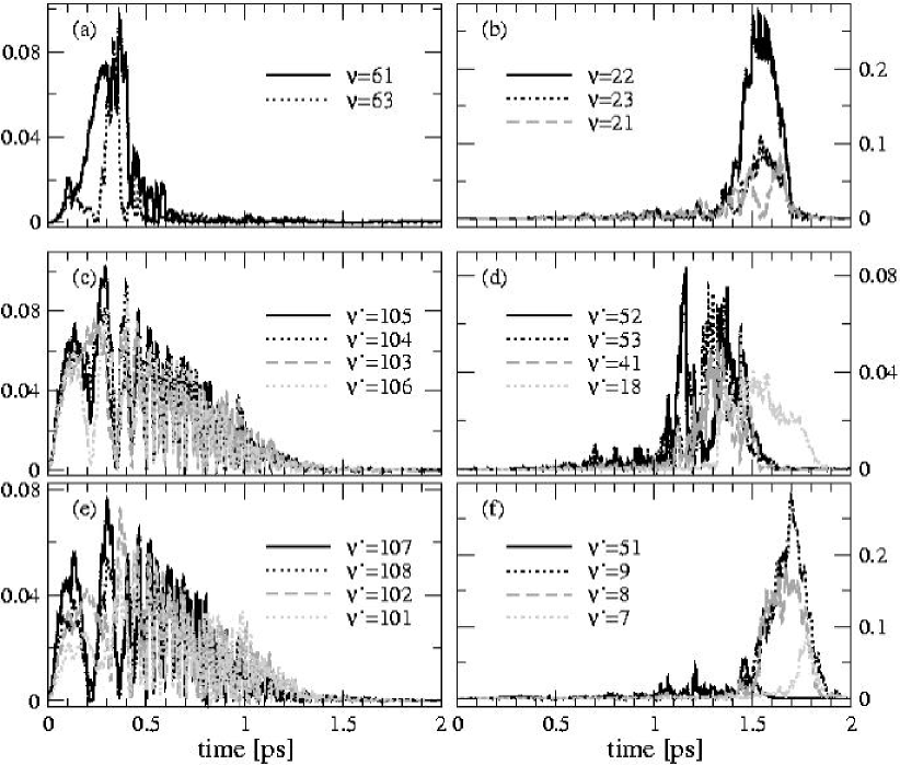
Figure 8: Vibrational level population of the dynamics with the optimal field for the electronically excited state (c)-(f) and the ground state (a)-(b)

The overall number of vibrational levels which get populated is 7 for the ground state ($v=62$ and $v=0$ have been plotted in Fig. 7 for better visibility) and 16 for the electronically excited state. For the ground state (Fig. 8 (a)-(b)), the two neighbouring levels of the initial state get populated at early times. At intermediate times, the population is spread over many different levels (and the continuum) while toward the end of the time interval, the population is concentrated in three levels ($v=21,22,23$). None of this levels is populated for more than 300 fs. This is the time which needs to be compared to the time scale of vibrational energy pooling. For the excited state (Fig. 8 (c)-(f)), the vibrational levels which get populated can be assigned to three different groups: At early times a number of levels ($v^{\prime}=101\ldots 108$) with good Franck-Condon overlap with the initial state get populated. While the population cycles back and forth between ground and excited state, these levels are overall populated for a comparatively long time. After about 1 ps, intermediate levels ($v^{\prime}=18,41,51\ldots 53$) are populated. Toward the end of the time interval the population is concentrated in levels ($v^{\prime}=7,8,9$) which have a very good Franck-Condon overlap with the target state, $v=0$. Also none of the excited state vibrational levels is populated for more than 300-400 fs which should be short enough to compete with vibrational energy pooling.

Note, that which specific vibrational levels are populated differs for different optimal pulses which are the result of initial guess pulses with different frequencies and intensities and of reduction of $T$ by different factors. The overall scheme of population, in particular for the excited state with the three groups at early, intermediate and long times, is found in all cases. This is not surprising because it simply reflects the fact that a multi-step scheme is needed to transfer a very weakly bound state to the vibrational ground state.

V Conclusions

We have shown that within a two-state model of Na₂ optimal fields which transfer highly excited vibrational states to the vibrational ground state to more than 99% can be found. We have performed calculations for moderately, highly and and extremely highly excited initial states ($v=10,40,62$ out of 66 bound levels). For moderately excited vibrational levels, a direct pathway from the initial to the target state exists, and a single central frequency in the guess field was sufficient to obtain an optimal field. For higher excited levels, a multistep scheme is required since initial and target state have good Franck-Condon overlap with different vibrational levels of the excited state. This was accounted for by assuming two central frequencies in the guess field. Experimentally, pulses with two central frequencies can be realized by sending a pulse with a single central frequency through a parametric amplifier.

The two control knobs of the optimization algorithm are the pulse intensity and the optimization time. A comparatively high intensity is needed to excite several quantum pathways whose interference constitutes the solution. The optimization time is usually chosen to correspond to the longest vibrational period of the system. We have explored ways to restrict both intensity and optimization time. This was possible by using information from optimal fields of a previous run of the algorithm with large intensity / long optimization time in the guess field which was used as input in a second run of the algorithm with smaller intensity and shorter optimization time. Optimal fields with integrated pulse energy on the order of milliJoule and overall duration on the order of a few picoseconds have thus been obtained.

The optimal control task we have investigated in this paper is much more difficult than those of previous control studies on the sodium dimer, such as populating certain ionization channels PaciJCP98 or displacing the ground state Gaussian wave packet ShenCPL03 . The fact that solutions could still be found, is due to the modification of the optimal control algorithm to calculate the change in field rather than the new field itself JosePRA03 . This ensures a smooth convergence of the field toward the optimal one and renders the algorithm very powerful.

We have neglected several possible loss channels. Two-photon transitions could populate an autoionizing state. However, since molecular autoionization occurs at small distances, the cross-sections are very small HuynhPRA98 . The field could moreover transfer angular momentum to the system thus exciting rotations. Both loss channels can be modelled by adding one or a few electronic states to the model. In general, additional channels do not necessarily pose a problem, they may even lead to more participating pathways improving the control PaciJCP98 . Intuitively, the field is able to avoid population of these loss channels if its phase is orthogonal to the transition dipole. It has been shown in local optimization calculations AllonJCP93 ; MalinovskyCPL97 , that this condition on the phase of the field can be used to lock the population in the desired channels. In global optimization, convergence can be facilitated by imposing a penalty on the loss channels SklarzPriv . Multiphoton ionization of the sodium atoms is more dangerous than excitation of rotations and molecular autoionization. It is rather likely to occur at the intensities we have found. Our calculations should therefore be repeated by adding an $N$-level Hamiltonian describing the atomic levels to the model. The task of the modified control problem is to transfer the vibrationally excited molecules to $v=0$ while avoiding population of the ionization loss channels at any time during the optimization interval. The latter has to be formulated as an additional constraint. The function $g(\varepsilon)$ does then also depend on the state $\varphi$, $g(\varepsilon,\varphi)$, and the equation for the new field has to be rederived. Work in this direction is in progress.

In a recent experiment XuPRL03 , ultracold Na₂ molecules have been produced from an atomic sodium condensate with the molecules occupying the $v=14$ vibrational level of the a${}^{3}\Sigma_{u}^{+}$ state. This vibrational level is very weakly bound ($<1$ cm^-1), and at such small binding energies the hyperfine interaction mixes singlet and triplet states SamuelisPRA00 . Note that in the asymptotic region the wave function of the triplet $v=14$ level is identical to that of the singlet $v=64$ level. The coupling between hyperfine states implies that also vibrational levels of the singlet state are populated, hence our results considering the X${}^{1}\Sigma_{g}^{+}$ should be applicable to the MIT experiment. Second, to obtain quantitative results our model should be improved to include all the states which are coupled by hyperfine interaction. This requires, however, several technical improvements and is therefore the subject of future work.

The MIT experiment raises another question regarding the feasibility of optimal control experiments with ultracold molecules. The reported lifetime of the molecular cloud is a few ms XuPRL03 . Conventional pulse shapers operate at about 1 kHz resulting in one cycle of the learning loop per millisecond. In standard control experiments a few thousand cycles can therefore be performed in a comparatively short time. If the MIT experiment were to be combined with a control scheme, only one or two cycles could be performed before the molecules are lost from the trap. It therefore seems necessary to provide more information from theoretical considerations than simply the required spectral bandwidth and intensity of the pulse. A promising approach has been suggested by de Vivie-Riedle and coworkers HornungJCP01 who defined the mask pattern of the optimal pulse by discrete Fourier transforms. Provided the calculated pulse is not too complex, this mask pattern can be directly fed into the pulse shaper avoiding the many cycles of a learning loop.

In addition to accounting for ionization losses and hyperfine interaction, our two-state model should be improved to consider rotations. This is particularly important because the molecules are not necessarily created with $J=0$ in the experiments using Feshbach resonances or three-body recombination. Since the rotational excitation is rather small, it will be sufficient to treat it by additional electronic states, for which the centrifugal barrier for each $J$ is added to the atom-atom interaction. One may speculate that some rotational excitation may even facilitate the stabilization process since the initial wave function due to the centrifugal barrier is more localized than the one for $J=0$.

Another possibility which leads to a more confined initial state for the stabilization process is given by forming the molecules by photoassociation. Two-color photoassociation or spontaneous emission after one-color photoassociation can directly populate levels around $v=40$. We have shown in our calculations that the optimal control task for such vibrational states which are still highly excited but already well-bound is much easier than for the last bound levels. The required intensities are hence more moderate (Cf. an integrated pulse energy of 1.5 mJ for $v=40$ vs. 4 mJ for $v=62$).

Finally, our calculations prompt the question whether spectrally simpler fields than those obtained in this study can be guessed. Our population analysis has shown that at least two cycles through the excited state are required. The first cycle populates excited state vibrational levels which have good Franck-Condon overlap with the initial state, and the second populates excited state vibrational levels with good Franck-Condon overlap with the target state. One could hence divide these steps, optimizing each separately. First calculations show that the intensities required for one such step are much lower than the ones completing the control task at once. Note that while the intensity is reduced, the overall time (including all steps) is prolonged. Another possibility is given by finding a solution for each of the steps intuitively without the optimal control algorithm, for example chirping the sequence of pulses. Furthermore, stabilization via optimal control could be combined with chirped pulse photoassociation JiriPRA01 ; Luc04 . For the Cesium dimer, it has been shown that a spatially focussed wave packet can be formed on the excited state Luc04 . To stabilize such a state to the ground vibrational level of the electronic ground state via OCT should also require comparatively little intensity. Our results furthermore indicate that STIRAP or any other adiabtic process is not likely to be a successful tool in transferring the highly excited molecules to the vibrational ground state. The multistep scheme implies that there is no direct adiabatic path, i.e. the Franck-Condon overlaps of a direct path are extremely small. Correspondingly, the intensity required for a direct adiabatic path is expected to be orders of magnitude larger than that obtained by us for an optimal field. Adiabaticity moreover requires the transfer to be slow. If we quantify slow as being at least one order of magnitude slower than the longest vibrational period of the problem, the process has to occur on the time scale of nanoseconds in the case of Na₂ and even longer times for heavier molecules. These are the time scales where loss processes become important and where condensate dynamics and molecular dynamics become entangled.

In conclusion, we have applied in this study optimal control theory to the stabilization of ultracold molecules. While we have started with a comparatively simple model, our present results point toward several directions of improvements which in turn correspond to different experimental schemes. We thus hope that the present work stimulates further research uniting the fields of cold molecules and optimal control.

Appendix A Brief review of Optimal control theory with the Krotov method

The Krotov method is one of several methods to derive an iterative algorithm which connects the objective of optimal control, calculated at the final time $t=T$, with the knowledge of the state of the system at intermediate times $0<t<T$. A general review was given in Ref. SklarzPRA02 , while a review for linear problems in the density matrix formalism was reported in Ref. JosePRA03 . In this paper, we need an even simpler version, that is the Krotov method for linear optimization of state-to-state transitions which we sketch in the following.

The equation of motion of the system is the Schrödinger equation,

$$\frac{\,\mathsf{d}}{\,\mathsf{d}t}|\varphi(t)\rangle=-\frac{i}{\hbar}\boldsymbol{\mathsf{\hat{H}}}(\varepsilon)|\varphi(t)\rangle\,,$$

whose right-hand-side is abbreviated by

$$|f(t,\varphi(t),\varepsilon)\rangle=-\frac{i}{\hbar}\boldsymbol{\mathsf{\hat{H}}}(\varepsilon)|\varphi(t)\rangle\,.$$ (9)

We omit the ket notation when just indicating the dependence on $|\varphi(t)\rangle$. The starting point is now the modified objective $J$ of Eq. (5), which is a functional of the state of the system and the field, $J[\varphi,\varepsilon]$. Due to integral term in Eq. (5), $J$ is a functional of the system’s state at all times, i.e. a functional of the system ”trajectory”. The problem is now to find conditions on $J$ which maximize the objective $F$.

To this end, one introduces an auxiliary functional $L[\varphi,\varepsilon;\Phi]$,

$$L[\varphi,\varepsilon;\Phi]=G(\varphi(T))-\Phi(0,\varphi_{i})-\int_{0}^{T}R(t,\varphi(t),\varepsilon)\,\mathsf{d}t$$ (10)

with

$$G(\varphi(T))=-F(\varphi(T))+\Phi(T,\varphi(T))\,,$$ (11)

$$R(t,\varphi(t),\varepsilon)=-g(\varepsilon)+\frac{\partial\Phi}{\partial t}+\mathfrak{Re}\left\langle\frac{\partial\Phi(t,\varphi(t))}{\partial\varphi}\bigg{|}f(t,\varphi(t),\varepsilon)\right\rangle$$ (12)

and $\Phi=\Phi(t,\varphi)$ an arbitrary continuously differentiable real function SklarzPRA02 ; JosePRA03 . Recall that $|\varphi_{i}\rangle=|\varphi(t=0)\rangle$, and $|\varphi_{f}\rangle$ is the target state. Note that the derivative of $\Phi$ with respect to the state means derivative with respect to both real and imaginary part of $|\varphi\rangle$, $|\frac{\partial}{\partial\varphi}\rangle=|\frac{\partial}{\partial\varphi_{R}}+i\frac{\partial}{\partial\varphi_{I}}\rangle$. If the state $|\varphi(t)\rangle$ and the field $\varepsilon(t)$ obey the Schrödinger equation, $R$ is given by $R=-g(\varepsilon)+\frac{\,\mathsf{d}\Phi}{\,\mathsf{d}t}$. It can then be shown SklarzPRA02 that $L[\varphi,\varepsilon;\Phi]=J[\varphi,\varepsilon]$ for any scalar function $\Phi$, i.e. the minimization of $J$ is equivalent to the minimization of $L$. In the latter one has complete freedom in the choice of $\Phi$. This property is used to construct an iterative algorithm. One first chooses $\Phi$ such that $L$ is maximum with respect to $|\varphi(t)\rangle$, i.e. the worst case. A new field is then derived from the condition of maximizing $R$ which in turn leads to minimization of $L$.

The first step (maximization of $L$) is equivalent to maximizing $G$ while minimizing $R$. This step is taken at the old state, $|\varphi(t)\rangle^{n}$. To simplify the equations, the maximum and mininum conditions are relaxed to extremum conditions. An additional condition in the end has then to ensure that the algorithm indeed improves the objective in each iteration. The extremum conditions are written as

$$\left|\frac{\partial R(t,\varphi(t),\varepsilon)}{\partial\varphi}\right\rangle_{|\varphi\rangle^{n}} = 0\,,$$ (13)

$$\left|\frac{\partial G(\varphi(T))}{\partial\varphi(T)}\right\rangle_{|\varphi\rangle^{n}} = 0\,.$$ (14)

The partial derivatives are again with respect to both real and imaginary part of $|\varphi\rangle$. Eq. (13) leads to

$$0 = \left|\frac{\partial}{\partial\varphi}\right\rangle\left[-g(\varepsilon)+\frac{\partial\Phi(t,\varphi(t))}{\partial t}+\mathfrak{Re}\left\langle\frac{\partial\Phi(t,\varphi(t))}{\partial\varphi}\bigg{|}f(t,\varphi,\varepsilon)\right\rangle\right]_{|\varphi\rangle^{n}}$$

$$= \frac{\partial}{\partial t}\left|\frac{\partial\Phi}{\partial\varphi}\right\rangle_{|\varphi\rangle^{n}}+\frac{1}{2}\left|\frac{\partial}{\partial\varphi}\right\rangle\left\langle\left(\frac{\partial\Phi}{\partial\varphi}\right)_{|\varphi\rangle^{n}}\bigg{|}f(t,\varphi,\varepsilon)\right\rangle+\frac{1}{2}\left\langle\left(\frac{\partial\Phi}{\partial\varphi}\right)_{|\varphi\rangle^{n}}\bigg{|}f(t,\varphi,\varepsilon)\right\rangle\bigg{\langle}\frac{\partial}{\partial\varphi}\bigg{|}$$

$$\;\;\;\;\;\;\;\;\;\;\;\;\;\;\;\;\;\;\;\;+\frac{1}{2}\left|\frac{\partial}{\partial\varphi}\right\rangle\left\langle f(t,\varphi,\varepsilon)\bigg{|}\left(\frac{\partial\Phi}{\partial\varphi}\right)_{|\varphi\rangle^{n}}\right\rangle+\frac{1}{2}\left\langle f(t,\varphi,\varepsilon)\bigg{|}\left(\frac{\partial\Phi}{\partial\varphi}\right)_{|\varphi\rangle^{n}}\right\rangle\bigg{\langle}\frac{\partial}{\partial\varphi}\bigg{|}\,.$$

Using that $|f\rangle=\,\mathsf{d}/\,\mathsf{d}t|\varphi\rangle$ and calculating $|\partial/\partial\varphi\rangle\langle f|$ from Eq. (9), we obtain

$$\frac{\,\mathsf{d}}{\,\mathsf{d}t}\left|\frac{\partial\Phi}{\partial\varphi}(t)\right\rangle_{|\varphi\rangle^{n}}=-\frac{i}{\hbar}\boldsymbol{\mathsf{\hat{H}}}^{+}(\varepsilon)\left|\frac{\partial\Phi}{\partial\varphi}(t)\right\rangle_{|\varphi\rangle^{n}}\,.$$ (15)

Eq. (14) together with the definition of $G(\varphi_{f})$ (Eq. 11)) gives

$$\left|\frac{\partial\Phi}{\partial\varphi}(T)\right\rangle_{|\varphi\rangle^{n}}=-\left|\frac{\partial F(\varphi)}{\partial\varphi}(T)\right\rangle\,.$$ (16)

Recall that $F$ is the original objective, and $|\partial F/\partial\varphi\rangle$ can thus be explicitly calculated. Eq. (15) can then be interpreted as first order differential equation for $|\gamma(t)\rangle=\left|\frac{\partial\Phi}{\partial\varphi}(t)\right\rangle_{|\varphi\rangle^{n}}$ with the ”initial” condition (at time $T$) given by Eq. (16). The knowledge of Eqs. (15) and (16) is therefore sufficient to determine $\Phi(t,\varphi)$ to first order in $|\varphi(t)\rangle$,

$$\Phi^{(1)}(t,\varphi)=\mathfrak{Re}\left\langle\left(\frac{\partial\Phi}{\partial\varphi}(t)\right)_{|\varphi\rangle^{n}}\bigg{|}\varphi(t)\right\rangle=\frac{1}{2}\left[\langle\gamma(t)\;|\varphi(t)\rangle+\langle\varphi(t)|\gamma(t)\rangle\right]\,\,.$$ (17)

From $\Phi^{(1)}$, $G$ and $R$ can be constructed to first order, $G^{(1)}$ and $R^{(1)}$. Thereby the first step of the algorithm for a linear optimization problem is completed. Note that $\Phi^{(1)}$ is never explicitly calculated, the equation of motion for $|\gamma(t)\rangle$ (Eq. (15)) will be solved instead.

To realize the second step, $R^{(1)}$ must be maximized with respect to the field. This step is supposed to lead to a new field, $\varepsilon^{n+1}$, which generates a new ”trajectory”, $|\varphi(t)\rangle^{n+1}$, according to the Schrödinger equation. We again relax the maximum to an extremum condition,

$$\frac{\partial R^{(1)}}{\partial\varepsilon}\bigg{|}_{\varepsilon^{n+1},|\varphi(t)\rangle^{n+1}}=0\,,$$ (18)

which gives

$$0 = \frac{\partial}{\partial\varepsilon}\left[-g(\varepsilon)+\frac{\partial\Phi^{(1)}}{\partial t}+\mathfrak{Re}\left\langle\frac{\partial\Phi^{(1)}}{\partial\varphi}\bigg{|}f(t,\varphi,\epsilon)\right\rangle\right]_{\varepsilon^{n+1},|\varphi(t)\rangle^{n+1}}$$

$$= -\frac{\partial g(\varepsilon)}{\partial\varepsilon}\bigg{|}_{\varepsilon^{n+1}}+\frac{1}{2}\left\langle\gamma(t)\bigg{|}\frac{\partial f(t,\varphi,\epsilon)}{\partial\varepsilon}\right\rangle_{\varepsilon^{n+1},|\varphi\rangle^{n+1}}+\frac{1}{2}\left\langle\frac{\partial f(t,\varphi,\epsilon)}{\partial\varepsilon}\bigg{|}\gamma(t)\right\rangle_{\varepsilon^{n+1},|\varphi\rangle^{n+1}}$$

and therefore

$$\frac{\partial g(\varepsilon)}{\partial\varepsilon}\bigg{|}_{\varepsilon^{n+1}}=\mathfrak{Re}\left\langle\gamma(t)\bigg{|}\frac{\partial f(t,\varphi,\epsilon)}{\partial\varepsilon}\right\rangle_{\varepsilon^{n+1},|\varphi\rangle^{n+1}}\,.$$ (19)

With our choice of the constraint $g(\varepsilon)$, Eq. (6), and using $\boldsymbol{\mathsf{\hat{H}}}=\boldsymbol{\mathsf{\hat{H}}}_{0}+\boldsymbol{\mathsf{\hat{\mu}}}\varepsilon(t)$ in the calculation of $|\partial f/\partial\varepsilon\rangle$ , we obtain for the new field

$$\varepsilon^{n+1}(t)=\varepsilon^{n}(t)+\frac{S(t)}{2\alpha}\mathfrak{Im}\left[\langle\gamma(t)|\boldsymbol{\mathsf{\hat{\mu}}}|\varphi(t)\rangle^{n+1}\right]\,.$$ (20)

The time evolution of the new state is given $|\varphi(t)\rangle^{n+1}=\boldsymbol{\mathsf{\hat{U}}}(t,0;\varepsilon^{n+1})|\varphi_{i}\rangle$, and $|\gamma(t)\rangle$ is obtained by formally solving Eq. (15), $|\gamma(t)\rangle=\boldsymbol{\mathsf{\hat{U}}}(t,T;\varepsilon^{n})|\gamma(T)\rangle$,

$$\varepsilon^{n+1}(t)=\varepsilon^{n}(t)+\frac{S(t)}{2\alpha}\mathfrak{Im}\left[\langle\gamma(T)|\boldsymbol{\mathsf{\hat{U}}}^{+}(t,T;\varepsilon^{n})\boldsymbol{\mathsf{\hat{\mu}}}\boldsymbol{\mathsf{\hat{U}}}(t,0;\varepsilon^{n+1})|\varphi_{i}\rangle\right]\,.$$

Using the definition of the objective $F$, Eq. (4), $|\gamma(T)\rangle$ is determined according to Eq. (16), $|\gamma(T)\rangle=c|\varphi_{f}\rangle$ with the coefficient

$$c=\langle\varphi_{f}|\varphi(T)\rangle^{n}=\langle\varphi_{f}|\boldsymbol{\mathsf{\hat{U}}}(T,0;\varepsilon^{n})|\varphi_{i}\rangle$$ (21)

and finally Eq. (III) is obtained.

Since we relaxed the maximum and mininum conditions to extremum conditions, we need to ensure that each iteration indeed improves the objective, $J[\varphi^{n},\varepsilon^{n}]-J[\varphi^{n+1},\varepsilon^{n+1}]\geq 0$,

$$J[\varphi^{n},\varepsilon^{n}]-J[\varphi^{n+1},\varepsilon^{n+1}] = L[\varphi^{n},\varepsilon^{n};\Phi^{(1)}]-L[\varphi^{n+1},\varepsilon^{n+1};\Phi^{(1)}]$$

$$= \Delta_{1}+\int_{0}^{T}\Delta_{2}(t)\,\mathsf{d}t$$

with

$$\Delta_{1} = G^{(1)}[\varphi(T)^{n}]-G^{(1)}[\varphi(T)^{n+1}]\,,$$

$$\Delta_{2}(t) = R^{(1)}[t,\varphi(t)^{n+1},\varepsilon^{n+1}]-R^{(1)}[t,\varphi(t)^{n},\varepsilon^{n}]\,,$$

A sufficient condition for $J[\varphi^{n},\varepsilon^{n}]-J[\varphi^{n+1},\varepsilon^{n+1}]\geq 0$ is $\Delta_{1},\Delta_{2}(t)\geq 0$. Constructing $G^{(1)}$ from Eq. (17), and using $|\gamma(T)\rangle=c|\varphi_{f}\rangle$ with Eq. (21) we see that

$$\Delta_{1}=\left|\langle\varphi_{i}|\boldsymbol{\mathsf{\hat{U}}}^{+}(T,0;\varepsilon^{n})-\boldsymbol{\mathsf{\hat{U}}}^{+}(T,0;\varepsilon^{n+1})|\varphi_{f}\rangle\right|^{2}\geq 0\,.$$ (22)

Because of the linearity of $f(t,\varphi,\varepsilon)$ w.r.t. $|\varphi\rangle$, $R^{(1)}(t,\varphi,\epsilon^{n})=-g(\varepsilon^{n})$ for any $|\varphi\rangle$, and we find

$$\Delta_{2}(t)=R^{(1)}[t,\varphi(t)^{n+1},\varepsilon^{n+1}]-R^{(1)}[t,\varphi(t)^{n+1},\varepsilon^{n}]\,.$$

Constructing $R^{(1)}$ from Eq. (17) and using again the linearity of the equation of motion, we obtain as condition for monotonous convergence

$$\Delta_{2}(t)=-g(\varepsilon^{1})+g(\varepsilon^{0})+\left(\varepsilon^{1}-\varepsilon^{0}\right)\frac{\partial g}{\partial\varepsilon}\Big{|}_{\varepsilon^{1}}\geq 0\,.$$ (23)

Eq. (19) and Eq. (23) are the central equations of the algorithm. The constraints which we formulate in $g(\varepsilon)$ must fulfill Eq. (23) to ensure convergence of the algorithm. Throughout this work we have used the constraint of restricted change in pulse energy, i.e. $g(\varepsilon)$ as given by Eq. (6), which respects Eq. (23) for all $\alpha$ as one can easily verify.

Appendix B Restriction of the spectral bandwidth

We tried other functional forms of the constraint $g(\varepsilon)$, in particular

$$g(\varepsilon)=\alpha_{1}(t)\left(\varepsilon-\varepsilon^{0}\right)^{2}-\alpha_{2}(t)\left(\varepsilon-\varepsilon^{\mathrm{ref}}\right)^{2}$$ (24)

with $\alpha_{i}=\alpha_{0i}/S(t)$, where the second term restricts the new field to a reference field $\varepsilon^{\mathrm{ref}}$ with a prespecified bandwidth (note, that the negative sign of this term implies maximization, i.e. the new field should be as close as possible to the reference field). Condition (23) is fulfilled for all $\alpha_{01}\geq\alpha_{02}\geq 0$. We found no effect for $\alpha_{02}\ll\alpha_{01}$ as not enough weight is put on the second constraint. Still 96% of the objective can be reached for $\alpha_{02}$ close to $\alpha_{01}$, but the spectral bandwidth is slightly reduced. In particular, spurious high-frequency components in the optimal puls can be avoided. The overall restriction of the bandwidth, however, appears to be insufficient.

In fact, it is not surprising that a condition formulated in time domain as Eq. (24) cannot achieve the desired control over a frequency domain property. This is a general problem of global (in time) optimal control schemes. Attempts to restrict the spectral bandwidth of the puls have been made before GrossJCP92 ; HornungJCP01 . However, this is possible only at the cost of monotonic convergence. An approach which unifies global optimal control with constraints in frequency domain will have to treat time and frequency on the same footing. This shall be the subject of future work.

References

- (1) E. A. Donley, N. R. Claussen, S. T. Thompson, and C. E. Wieman, Nature 417, 529 (2002)
- (2) C. A. Regal, C. Ticknor, J. L. Bohn, and D. S. Jin, Nature 424, 47 (2003)
- (3) J. Herbig, T. Kraemer, M. Mark, T. Weber, C. Chin, H.-C. Nägerl, and R. Grimm, Science 301, 1510 (2003)
- (4) S. Dürr, T. Volz, A. Marte, and G. Rempe, Phys. Rev. Lett. 92, 020406 (2004)
- (5) K. Xu, T. Mukaiyama, J. R. Abo-Shaeer, J. K. Chin, D. Miller, and W. Ketterle, Phys. Rev. Lett. 91, 210402 (2003)
- (6) S. Jochim, M. Bartenstein, A. Altmeyer, G. Hendl, S. Riedl, C. Chin, J. Hecker Denschlag, and R. Grimm, Science (2003)
- (7) M. Greiner, C. A. Regal, and D. S. Jin, Nature 426, 537 (2003)
- (8) M. W. Zwierlein, C. A. Stan, C. H. Schunck, S. M. F. Raupach, S. Gupta, Z. Hadzibabic, and W. Ketterle, Phys. Rev. Lett. 91, 250401 (2003)
- (9) N. Vanhaecke, W. de Souza Melo, B. L. Tolra, D. Comparat, and P. Pillet, Phys. Rev. Lett. 89, 063001 (2002)
- (10) C. Chin, A. J. Kerman, V. Vuletić, and S. Zhu, Phys. Rev. Lett. 90, 033201 (2003)
- (11) F. Masnou-Seeuws and P. Pillet, Adv. in At., Mol. and Opt. Phys. 47, 53 (2001)
- (12) E. Timmermans, P. Tommasini, M. Hussein, and A. Kerman, Phys. Rep. 315, 199 (1999)
- (13) G. Meijer, ChemPhysChem 3, 495 (2002)
- (14) N. Balakrishnan, N. C. Forrey, and A. Dalgarno, Phys. Rev. Lett. 80, 3224 (1998)
- (15) P. Soldán, M. T. Cvitaš, J. M. Hutson, P. Honvault, and J.-M. Launay, Phys. Rev. Lett. 89, 153201 (2002)
- (16) C. E. Treanor, J. W. Rich, and R. G. Rehm, J. Chem. Phys. 48, 1798 (1967)
- (17) S. A. Rice and M. Zhao, Optimal Control of Molecular Dynamics, Wiley, New York, 2000
- (18) T. Brixner and G. Gerber, ChemPhysChem 4, 418 (2003)
- (19) M. Mackie, R. Kowalski, and J. Javanainen, Phys. Rev. Lett. 86, 3803 (2000)
- (20) P. D. Drummond, K. V. Kheruntsyan, D. J. Heinzen, and R. H. Wynar, Phys. Rev. A 65, 063619 (2002)
- (21) T. Hornung, S. Gordienko, R. de Vivie-Riedle, and B. J. Verhaar, Phys. Rev. A 66, 043607 (2002)
- (22) S. E. Sklarz and D. J. Tannor, Phys. Rev. A 66, 053619 (2002)
- (23) V. Ramakrishna, M. V. Salapaka, M. Dahleh, H. Rabitz, and A. Peirce, Phys. Rev. A 51, 960 (1995)
- (24) G. Huang, T. Tarn, and J. Clark, J. Math. Phys. 24, 2608 (1983)
- (25) M. Elbs, H. Knöckel, T. Laue, C. Samuelis, and E. Tiemann, Phys. Rev. A 59, 3665 (1999)
- (26) T. Baumert, B. Bühler, R. Thalweiser, and G. Gerber, Phys. Rev. Lett. 64, 733 (1990)
- (27) A. Shnitman, I. Sofer, I. I. Golub, A. Yogev, M. Shapiro, Z. Chen, and P. Brumer, Phys. Rev. Lett. 76, 2886 (1996)
- (28) C. McKenzie, J. Hecker Denschlag, H. Häffner, A. Browaeys, L. E. E. de Araujo, F. K. Fatemi, K. M. Jones, J. E. Simsarian, D. Cho, A. Simoni, E. Tiesinga, P. S. Julienne, K. Helmerson, P. D. Lett, S. L. Rolston, and W. D. Phillips, Phys. Rev. Lett. 88, 120403 (2002)
- (29) A. Vardi, D. Abrashkevich, E. Frishman, and M. Shapiro, J. Chem. Phys. 107, 6166 (1997)
- (30) M. Machholm and A. Suzor-Weiner, J. Chem. Phys. 105, 971 (1996)
- (31) J. Paci, M. Shapiro, and P. Brumer, J. Chem. Phys. 109, 8993 (1998)
- (32) Z. Shen and V. Engel, Chem. Phys. Lett. 358, 344 (2002)
- (33) A. Bartana, R. Kosloff, and D. J. Tannor, J. Chem. Phys. 99, 196 (1993)
- (34) J. P. Palao and R. Kosloff, Phys. Rev. Lett. 89, 188301 (2002)
- (35) A. Bartana, R. Kosloff, and D. J. Tannor, J. Chem. Phys. 106, 1435 (1997)
- (36) A. Bartana, R. Kosloff, and D. J. Tannor, Chem. Phys. 267, 195 (2001)
- (37) J. P. Palao and R. Kosloff, Phys. Rev. A 68, 062308 (2003)
- (38) P. Naidon and F. Masnou-Seeuws, Phys. Rev. A 68, 033612 (2003)
- (39) C. Samuelis, E. Tiesinga, T. Laue, M. Elbs, H. Köckel, and E. Tiemann, Phys. Rev. A 63, 012710 (2000)
- (40) E. Tiemann, H. Köckel, and H. Richling, Z. Phys. D. 37, 323 (1996)
- (41) P. Pellegrini and O. Dulieu, In preparation
- (42) M. Marinescu and A. Dalgarno, Phys. Rev. A 52, 311 (1995)
- (43) V. Kokoouline, O. Dulieu, R. Kosloff, and F. Masnou-Seeuws, J. Chem. Phys. 110, 9865 (1999)
- (44) K. Willner, O. Dulieu, and F. Masnou-Seeuws, J. Chem. Phys. 120, 548 (2003)
- (45) R. Kosloff, Annu. Rev. Phys. Chem. 45, 145 (1994)
- (46) R. Kosloff, Quantum Molecular Dynamics on Grids, in Dynamics of Molecules and Chemical Reactions, edited by R. Wyatt and J. Zhang, pages 185–230, Marcel Dekker, New York, 1996
- (47) T. Hornung, M. Motzkus, and R. de Vivie-Riedle, Phys. Rev. A 65, 021403 (2002)
- (48) B. Huynh, O. Dulieu, and F. Masnou-Seeuws, Phys. Rev. A 57, 958 (1998)
- (49) V. S. Malinovsky, C. Meier, and D. J. Tannor, Chem. Phys. Lett. 221, 67 (1997)
- (50) S. E. Sklarz and D. J. Tannor, Private Communication
- (51) T. Hornung, M. Motzkus, and R. de Vivie-Riedle, J. Chem. Phys. 115, 3105 (2001)
- (52) J. Vala, O. Dulieu, F. Masnou-Seeuws, P. Pillet, and R. Kosloff, Phys. Rev. A 63, 013412 (2001)
- (53) E. Luc-Koenig, R. Kosloff, F. Masnou-Seeuws, and M. Vatasescu, Photoassociation of cold atoms with chirped laser pulses: time-dependent calculations and analysis of the adiabatic transfer within a two-state model, In preparation
- (54) P. Gross, D. Neuhauser, and H. Rabitz, J. Chem. Phys. 96, 2834 (1992)