Collective excitations in circular atomic configurations, and single-photon traps

Abstract

Correlated excitations in a plane circular configuration of identical atoms with parallel dipole moments are investigated. The collective energy eigenstates, which are formally identical to Frenkel excitons, can be computed together with their level shifts and decay rates by decomposing the atomic state space into carrier spaces for the irreducible representations of the symmetry group $\mathbb{Z}_{N}$ of the circle. It is shown that the index $p$ of these representations can be used as a quantum number analogously to the orbital angular momentum quantum number $l$ in hydrogen-like systems. Just as the hydrogen $s$-states are the only electronic wave functions which can occupy the central region of the Coulomb potential, the quasi-particle corresponding to a collective excitation of the atoms in the circle can occupy the central atom only for vanishing $\mathbb{Z}_{N}$ quantum number $p$. If a central atom is present, the $p=0$ state splits into two and shows level-crossing at certain radii; in the regions between these radii, damped quantum beats between two ”extreme” $p=0$ configurations occur. The physical mechanisms behind super- and subradiance at a given radius are discussed. It is shown that, beyond a certain critical number of atoms in the circle, the lifetime of the maximally subradiant state increases exponentially with the number of atoms in the configuration, making the system a natural candidate for a single-photon trap.

I Introduction

When a collection of identical atoms is located such that their mutual distances are comparable to the wavelength of an atomic transition, the mode structure of the electromagnetic field is altered, at least for photon states whose energy lies in the neighbourhood of the associated atomic transition; at the same time, level shifts and spontaneous emission rates of the states in the atomic ensemble undergo changes. Furthermore, the atoms in the sample become entangled with each other as well as with the radiation field via photon exchange. The sample then occupies collective states whose associated spontaneous emission rates can be greater or smaller than the single-atom decay rate and are called super- or subradiant, accordingly. For a collection of two-level atoms, this phenomenon was discovered as early as 1954 by Dicke Dicke (1954).

Super- and subradiance in the near-field regime has been studied by a number of authors. Reviews of the subject were given in Gross and Haroche (1982); Benedict et al. (1996). The theory of subradiance in particular was treated in a four-paper series in Crubellier et al. (1985); Crubellier and Pavolini (1986); Crubellier et al. (1987); Crubellier and Pavolini (1987). Wigner functions, squeezing properties and decoherence of collective states in the near-field regime have been presented in Benedict et al. (1996); Benedict and Czirják (1999); Földi et al. (2002), while triggering of sub- and superradiant states was shown to be possible in Keitel et al. (1992). Experimentally, super- and subradiance have been observed in Pavolini et al. (1985); DeVoe and Brewer (1996).

In all these investigations the so-called ”small-sample approximation” played a crucial role: Here the atoms are assumed to be so close together that they are all subject to the same phase of the radiation field. ”Closeness” here is measured on a length scale whose unit is the wavelength $\lambda$ of the dominant atomic transition under consideration. The small-sample approximation is then manifested by using an interaction Hamiltonian which is independent of the spatial location of the constituents, similar to a long-wavelength approximation. Thus, in this approximation, super- and subradiance appears to be a near-field phenomenon.

In this paper we perform a detailed investigation of the simply-excited correlated states observed in a planar circular configuration of atoms beyond the small-sample approximation: That is to say, we determine the level shifts and decay properties of correlated states for atomic ensembles in configurations with arbitrary radius of the circle, not restricted to the small-sample limit. The simply-excited correlated states so obtained turn out to be formally identical to Frenkel excitons, e.g., in a molecular crystal. Conceptually, however, Frenkel excitons differ from our collective excitations in that the former are usually thought of as being mediated by the interatomic Coulomb interaction only Frenkel (1931); Davydov (1971); Knox (1963); Kenkre and Reineker (1982), whereas, in the latter case, the delocalization of the excitation energy occurs through the exchange of transverse photons and therefore proceeds through radiative processes. Below we shall comment on this conceptual difference in greater detail.

Taking advantage of the discrete rotational symmetry $\mathbb{Z}_{N}$ of the circle, the complex eigenvalues and eigenstates of the non-Hermitean channel Hamiltonian governing the dynamics in the radiationless subspace of the system can be determined analytically by group-theoretical methods. The physical mechanism determining super- or subradiance of a given eigenstate is then discussed. In particular we show that each of the collective eigenstates has certain ranges of the radius of the circle for which it can be the maximally super- or subradiant state. We demonstrate that, for an ensemble with $N$ outer atoms in the circle, there are $(N-1)$ states which are insensitive to the presence of a central atom; this means that the associated wavefunctions, level shifts and decay rates of the quasi-particle describing the collective excitation do not change when the atom at the center is removed, simply because the latter is not occupied. There are only two states in a circular ensemble which occupy the central atom; we show that they are analogues of the $s$-state wave functions in hydrogen-like systems: Just as the $s$ states carry angular momentum quantum number $l=0$ and therefore transform under the identity representation of $SO(3)$, our collective $p=0$ states correspond to the identity representation of the symmetry group $\mathbb{Z}_{N}$; and just as the $s$ states are the only ones which are nonvanishing at the center-of-symmetry of the Coulomb potential in a hydrogen-like system, so are our $p=0$ states the only quasi-particle states which occupy the central atom at the center-of-symmetry of the circle. These two $p=0$ states for the configuration with central atom exhibit quantum beats between two extreme configurations, one, in which only outer atoms are occupied, the other, in which only the central atom is excited. At certain radii the two levels cross, and no quantum beats occur; in this case the population transfer between the two extreme configurations is completely aperiodic. For other radii, the beat frequency is so much smaller than the decay rate of the collective state as a whole, that the decay effectively proceeds like an aperiodic ”population swap”. Finally we show numerically that, by increasing the number of atoms in the circle for fixed radius, we arrive at a domain where the minimal spontaneous decay rate in the sample decreases exponentially with the number of atoms in the circle. Such configurations therefore are natural candidates for single-photon traps. This pronounced photon trapping may even survive in the presence of dephasing interactions with an environment, or more generally, when the system is subject to a (moderate) loss of quantum coherence due to external noise.

II Spontaneous Decay and Level Shifts in a Sample of Correlated Atoms

In this work we do not study the most general collective states in an atomic ensemble but focus on those states which are coupled to one resonant photon only; we shall call these states simply-excited. The simply-excited uncorrelated states of the sample are given as $|e_{1},g_{2},\cdots,g_{N},0\rangle\equiv|1,0\rangle$, $\ldots$, $|g_{1},g_{2},\cdots,e_{N},0\rangle\equiv|N,0\rangle$, where $|g_{A}\rangle$, $|e_{A}\rangle$ denote the ground and excited level of the $A$th atom, and $|0\rangle$ is the radiative vacuum. These states are coupled to the continuum of one-photon states $|g_{1},g_{2},\cdots,g_{N},{\bf k}s\rangle\equiv|G,\mathbf{k}s\rangle$, where $({\bf k}s)$ denote the wave vector and polarization of the photon. The uncorrelated states $|A,0\rangle$ are occupied by a sample of atoms for which the following is true: 1.) the atoms have infinite mutual distance; and 2.) precisely one of the $N$ atoms is excited.

If we now think of adiabatically decreasing the spatial separation of the atoms to finite distances, the atoms will begin to ”feel” each other via their mutual Coulomb (dipole-dipole) interaction and their coupling to the radiation field, and the states $|A,0\rangle$ will no longer be the stationary energy eigenstates. Rather, we expect that superpositions of uncorrelated excitations will emerge,

$$\left|\mathcal{C}\right\rangle=\sum_{B=1}^{N}c_{B}\,|B,0\rangle\quad,$$ (1)

with coefficients $c_{B}$ which are obtained by diagonalization of a suitable effective Hamiltonian, given below.

Inherent in our model is the assumption that the atoms taking part in the collective excitation have mutual distances on the order of magnitude of an optical wavelength, i.e., several hundred nanometers. As a consequence, electronic wavefunctions pertaining to different atoms do not overlap, and we can refrain from antisymmetrization of the total electronic state (Slater determinant). This justifies the use of product states for the simply-excited uncorrelated states $\left|A,0\right\rangle$. Furthermore, it is clear that under these conditions, the migration of excitation energy between the different atoms can proceed only through the exchange of transverse photons, as the Coulomb dipole-dipole interaction will play a role only for interatomic distances $R_{AB}\ll\lambda_{eg}$, where $\lambda_{eg}$ is the dominant wavelength of the Bohr transition. This feature seems to set the correlated states (1) apart from the usual notion of Frenkel excitons Frenkel (1931); Davydov (1971); Knox (1963); Kenkre and Reineker (1982), although both are formally identical in being superpositions of simply-excited product states. In the case of a Frenkel exciton, however, it is usually assumed that the atoms involved in the collective excitation are located on the lattice sites of a crystal and therefore have mutual distances comparable to a Bohr radius. In this case, the “excitation transfer interaction” Knox (1963) responsible for the migration of excitation energy is Coulombic, and indeed this is assumed in all standard accounts on Frenkel excitons (Coulomb means direct plus exchange interaction, if relevant). To quote from a standard reference (Davydov (1971), p. 19), “Excitons … are idealized elementary excitations in whose consideration we ignore the delay effects and take into account only Coulomb interaction”. This points out an important conceptual difference between our collective excitations and the standard notion of a Frenkel exciton.

We can express this difference in even greater detail: In the case of the “traditional” Frenkel exciton, the system under consideration is comprised of the totality of atoms in the crystal, interacting through the instantaneous Coulomb potential or its multipolar approximation. On account of this interaction, the atoms become entangled with each other, but certainly remain unentangled with the transverse degrees of freedom of the radiation field, at least as long as only quasi-resonant atom-photon interactions (rotating-wave approximation) are taken into account. On the other hand, the collective states considered in our work here are states of the total system atoms+radiation, and as a consequence, in any of these states the atoms must be regarded as being entangled not only with each other but also with the transverse radiative degrees of freedom. This entanglement, of course, is a direct consequence of the fact that the migration of excitation energy proceeds through exchange of a transverse photon: the excited atom $A$ emits a quasi-resonant photon which, in turn, gets absorbed by atom $B$, thereby exciting the latter. The electrostatic interaction plays a role in this process only for interatomic distances which are small compared to an optical wavelength. Due to these conceptual differences, we hesitate to call our collective states Frenkel excitons.

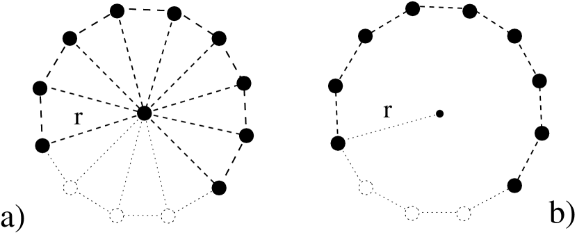
Figure 1: The two circular configurations of $N(+1)$ atoms which are examined: In configuration a), $N$ outer atoms form a regular $N$-polygon with radius $r$, plus an atom at the center. Configuration b) is the same as a), but without the central element.

We now present the details of the computation: Let $N$ neutral atoms be labelled by $A=1,2,\ldots,N$, each atom being localized around a fixed point $\mathbf{R}_{A}$ in space, where $\mathbf{R}_{A}$ are $c$-numbers, not operators. The atoms are assumed to be identical, infinitely heavy, and having a spatial extent on the order of magnitude of a Bohr radius $a_{0}$. The point charges within each ensemble are labelled as $q_{A\alpha}$. On taking the long-wavelength approximation in the minimal-coupling Hamiltonian and performing the Göppert-Mayer transformation we arrive at the electric-dipole Hamiltonian

$$H=\sum_{A}\sum_{\alpha}\frac{\mathbf{p}_{A\alpha}^{2}}{2\,m_{A\alpha}}+\sum_{A}\sum_{\alpha<\beta}V_{A\alpha\beta}+\sum_{j}\hbar\omega_{j}a_{j}^{{\dagger}}a_{j}-$$ (2a)

$$-\sum_{A}\mathbf{d}_{A}\bullet\mathbf{E}_{\bot}(\mathbf{R}_{A})=H_{0}+H_{I}\quad,$$ (2b)

where the unperturbed Hamiltonian $H_{0}$, given in (2a), contains the sum over atomic Hamiltonians $H_{0A}$ including the Coulomb interaction $V_{A\alpha\beta}$ between the internal constituents of atoms $A=1,\ldots,N$, but without the Coulomb dipole-dipole interaction $V^{\text{dip}}_{AB}$ between atoms $A$ and $B$, for $A\neq B$; and the normally-ordered radiation operators. The electric-dipole interaction is given in (2b), where $\mathbf{E}_{\bot}$ denotes the transverse electric field operator. The interatomic Coulomb dipole-dipole interaction $V^{\text{dip}}_{AB}$ seems to be conspicuously absent in (2); however, it is a feature of the Göppert-Mayer transformation to transform this interaction into a part of the transverse electric field, so that the Coulomb interaction will emerge as a factor in the level-shift operator, as will be seen below in formulae (8–9). As a consequence of being a part of the transverse electric-field operator, the interatomic Coulomb interaction is now fully retarded, in contrast to the instantaneous Coulomb interaction in the minimal-coupling Hamiltonian.

The process we study in this work consists of the radiative decay of a simply-excited correlated atomic state, or a “Frenkel exciton”, which is resonantly coupled to a continuum of one-photon states. For this reason, two-photon- or higher-photon-number processes can be expected to play a negligible role, so that it is admissible to truncate the possible quantum states of the radiation field to one-photon states $\left|\mathbf{k}s\right\rangle$, and the vacuum $|0\rangle$. The rotating-wave approximation is now taken Loudon (1983), Thus, amongst the admissible single-photon transitions $\left|\mathcal{C}\right\rangle\rightarrow\left|G,\mathbf{k}s\right\rangle$ and $\left|\mathcal{C}\right\rangle\rightarrow\left|AB,\mathbf{k}s\right\rangle$, only processes of the first kind are taken into account. The radiationless subspace $Q$ is spanned by the states $\left|A,0\right\rangle$, using the same symbol for the associated projector $Q=\sum_{A=1}^{N}\left|A,0\right\rangle\left\langle A,0\right|$, while $P$ denotes the projector onto the subspace of one-photon states $\left|G,\mathbf{k}s\right\rangle$.

In the present scenario we assume that the system atoms+radiation is closed and therefore evolves unitarily; a qualitative consideration of the impact of dephasing interactions will be given in the last section VII. If, at time $t=0$, the system is in a correlated state (1), the probability of finding the radiation at $t>0$ to be still trapped in the system is determined by the $Q$-space amplitudes

$$\begin{gathered}\left\langle A,0\right|U(t,0)\left|\mathcal{C}\right\rangle=-\sum_{B=1}^{N}\frac{1}{2\pi i}\int dE\;e^{-\frac{i}{\hbar}Et}\;\cdot\\ \cdot\left\langle A,0\right|\,QG(E_{+})Q\,\left|B,0\right\rangle\;c_{B}\quad,\end{gathered}$$ (3)

where the $Q$-space Green operator $QG(E_{+})Q$ is given in terms of the non-Hermitean $Q$-channel Hamiltonian $\mathcal{H}(E_{+})$ as $QG(E_{+})Q=1/(E_{+}-\mathcal{H}(E_{+}))$. At the initial energy $E_{i}=E_{e}+(N-1)E_{g}$, where $E_{e},E_{g}$ are the energies of the excited and ground state of a single atom, we have

$$\mathcal{H}(E_{i+})=QH_{0}Q+\hbar\Delta(E_{i})-i\,\frac{\hbar}{2}\,\Gamma(E_{i})\quad,$$ (4)

where $\Delta(E_{i})$ is the level-shift operator

$$\Delta_{AB}(E_{i}) =-\frac{1}{2}\Gamma\,S(X)\quad,\quad X=k_{eg}R_{AB}$$ (5a)

$$S(X) =\frac{3}{2}\left\{\frac{\cos X}{X}-\frac{\sin X}{X^{2}}-\frac{\cos X}{X^{3}}+\right.$$

$$+\left.\frac{1}{\pi X^{2}}\int\limits_{0}^{\infty}du\;\frac{e^{-u}\left(1+u+u^{2}\right)}{u^{2}+X^{2}}\right\}\quad.$$ (5b)

and $\Gamma(E_{i})$ is the decay operator

$$\Gamma_{AB}(E_{i}) =\Gamma\,D_{1}(k_{eg}R_{AB})\quad,$$ (6a)

$$D_{1}(X) =\frac{3}{2}\left(\frac{\sin X}{X}+\frac{\cos X}{X^{2}}-\frac{\sin X}{X^{3}}\right)\quad,$$ (6b)

in the $Q$-space, where $\Gamma=d^{2}k_{eg}^{3}/(3\pi\epsilon_{0}\hbar)$ is the spontaneous emission rate of a single atom in a radiative vacuum and $E_{eg}=E_{e}-E_{g}=\hbar ck_{eg}$. The level-shift function $S$ can be approximated by

$$\begin{gathered}S(X)_{\text{approx}}\simeq\frac{3}{2}\left\{\frac{\cos X}{X}-\frac{\sin X}{X^{2}}-\frac{\cos X}{X^{3}}+\right.\\ +\left.\frac{1}{\pi X^{2}}\left[\frac{1-X^{2}}{X}\,\arctan\frac{1}{X}+1+\frac{1}{2}\,\ln\frac{1+X^{2}}{X^{2}}\right]\right\}\quad.\end{gathered}$$ (7)

A plot of the functions $D_{1}$, $S$ and $S_{\text{approx}}$ is given in Fig. 2.

[Remark: In the more general case of arbitrarily aligned atoms there are two correlation functions $D_{1},D_{2}$ emerging in the decay matrix rather than just one. This is indicated by our denotation. For parallely aligned atoms, the contribution of $D_{2}$ vanishes.]

A function similar to $D_{1}$, but within a classical context, is the dyadic Green function of the electromagnetic field de Vries et al. (1998).

The off-diagonal elements of the level-shift matrix $\Delta_{AB}$ can be put into the form

$$\Delta_{AB}(E_{i})=\frac{d^{2}}{4\pi\epsilon_{0}\hbar}\frac{1}{R_{AB}^{3}}\;f(R_{AB})\quad,$$ (8)

where $f(R_{AB})$ is an analytic function of $R_{AB}$ which tends to $\frac{1}{2}$ as $R_{AB}$ tends to zero. Comparison with the Coulomb dipole-dipole interaction between the two atoms $A$ and $B$,

$$V^{\text{dip}}_{AB}=\frac{\mathbf{d}_{A}\bullet\mathbf{d}_{B}-3\,\left(\mathbf{d}_{A}\bullet\mathbf{e}_{AB}\right)\left(\mathbf{d}_{B}\bullet\mathbf{e}_{AB}\right)}{4\pi\epsilon_{0}\,R_{AB}^{3}}=\frac{d^{2}}{4\pi\epsilon_{0}\,R_{AB}^{3}}$$ (9)

shows that the level shifts indeed contain the dipole-dipole Coulomb interaction between the charged ensembles $A$ and $B$. On the other hand, the diagonal elements of $\Delta_{AB}$ diverge due to Coulomb and radiative self-energy; to remove this deficiency we renormalize Bjorken and Drell (1990a, b); Bogoliubov and Shirkov (1959); Itzykson and Zuber (1980); Ryder (1996); Bailin and Love (1986) the initial energy (“bare” energy) by redefining

$$E_{i}\longrightarrow E_{i}+\lim\limits_{X\rightarrow 0}\hbar\Delta_{AA}(E_{i})\equiv\widetilde{E}_{i}\quad,$$ (10)

and subtracting the same infinity from the level-shift matrix,

$$\Delta_{AB}(E_{i})\longrightarrow\widetilde{\Delta}_{AB}(E_{i})\equiv\begin{cases}\quad\Delta_{AB}(E_{i})&,\quad A\neq B\;,\\ \quad 0&,\quad A=B\;,\end{cases}$$ (11)

where $\widetilde{E}_{i}$ is now assumed to have a finite value, namely the value unperturbed by the presence of $N-1$ other atoms; as a consequence, $E_{i}$ must be assumed to have been infinite in the first place. The only observable level-shifts are now those due to interatomic interactions.

The $Q$-channel Hamiltonian in the uncorrelated basis now becomes

$$\left\langle A,0\right|\mathcal{H}(E_{i})\left|B,0\right\rangle=\widetilde{E}_{i}\,\Eins_{N}-\frac{\hbar\Gamma}{2}\,\mathcal{R}\quad,$$ (12a)

$$\mathcal{R}=\left(\begin{array}[]{*3{c}}i&S+iD_{1}&\cdots\\ S+iD_{1}&i&\cdots\\ \vdots&\vdots&\ddots\end{array}\right)=\mathcal{R}^{T}\quad.$$ (12e)

This matrix can be diagonalized in terms of left and right eigenvectors Morse and Feshbach (1953)

$$\begin{gathered}\left\langle A,0\right|\mathcal{H}(E_{i})\left|B,0\right\rangle=\\ \ =\sum_{p=1}^{N}\left\langle A,0\right|\left.\mathcal{C}_{p}\right\rangle\bigg{\{}\widetilde{E}_{i}-\frac{\hbar\Gamma(k_{eg})}{2}\,\mu_{p}\bigg{\}}\left\langle\mathcal{C}_{p}^{*}\right|\left.B,0\right\rangle\quad.\end{gathered}$$ (13)

where

$$\widetilde{\Delta}_{p} =-\frac{\Gamma}{2}\;\mathfrak{Re}\!~{}\mu_{p}\quad,$$ (14a)

$$\Gamma_{p} =\hskip 7.22212pt\Gamma\;\mathfrak{Im}\!~{}\mu_{p}\quad,$$ (14b)

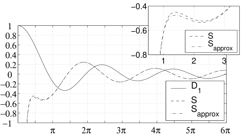
Figure 2: Plots of the correlation functions $D_{1}(X)$ and $S(X)$ responsible for spontaneous decay (”D”) and level shifts (”S”), respectively. $X$ is equal to $2\pi$ times the interatomic distance measured in units of the wavelength $\lambda_{eg}$ of the dominant atomic transition. $D_{1}$ becomes maximal at zero interatomic distance while $S$ tends to minus infinity there, due to Coulomb- and radiative self-energy of the atomic dipole. Both functions tend to zero as $X\rightarrow\infty$, expressing the fact that any kind of correlation must cease to exist for infinite distance. The inset shows a comparison between the exact shift function $S(X)$, based on eq. (5b), and the approximation $S_{\text{approx}}$, based on eq. (7).

For the given radius $r$, number of atoms $N$, and configuration (a) or (b), let $\left|\mathcal{C}_{{\text{min}}}\right\rangle$ be the eigenstate with the smallest decay rate,

$$\Gamma_{\text{min}}\leq\Gamma_{p}\quad\text{for all $p=1,\ldots,N$}\quad.$$ (15)

Then the associated correlated state

$$\left|\mathcal{C}\right\rangle=\frac{1}{\sqrt{\left\langle\mathcal{C}_{{\text{min}}}|\mathcal{C}_{{\text{min}}}\right\rangle}}\,\left|\mathcal{C}_{{\text{min}}}\right\rangle\quad$$ (16)

is the most stable one with respect to spontaneous decay [saying nothing about stability against environmental perturbations], and hence is a candidate for a single-photon trap.

III Cyclic symmetry of the circular atomic configurations

We now construct the eigenvectors $\left|\mathcal{C}_{p}\right\rangle$ of $\mathcal{H}(E_{i})$ explicitly by group-theoretical means, taking advantage of the fact that the system has a cyclic symmetry group

$$G =\left\{e,T,T^{2},\ldots,T^{N-1}\right\}\quad,$$ (17a)

$$T^{N} =e\quad,$$ (17b)

where $N$ is the number of outer atoms along the perimeter of the circle, the generator $T$ acts on coordinate space as a (passive) rotation by the angle $2\pi/N$ about the symmetry axis of the circle, and acts on the state space unitarily by relabelling the outer atoms, but leaving the central atom invariant,

$$T\,\left|A\right\rangle =\left|A-1\right\rangle\quad,$$ (18)

$$T\,\left|z\right\rangle =\left|z\right\rangle\quad.$$

The unitary irreducible representations of $\mathbb{Z}_{N}$ are given by

$$\Gamma^{p}\left(T^{A}\right)=\exp\left(\frac{2\pi ipA}{N}\right)\quad,\quad A=1,2,\ldots,N\quad,$$ (19)

and using appropriate projection operators, the radiationless $Q$-space can be decomposed into an orthogonal direct sum $Q=\oplus_{p=0}^{N-1}\mathsf{T}_{p}$ of carrier spaces $\mathsf{T}_{p}$ of irreducible representations $\Gamma^{p}$. Since the channel Hamiltonians of both configurations are invariant under this transformation,

$$T^{-1}\,\mathcal{H}\,T=\mathcal{H}\quad,$$ (20)

$\mathcal{H}$ preserves all carrier spaces $\mathsf{T}_{p}$ and hence can be diagonalized on each $\mathsf{T}^{p}$ separately. This simplification makes it possible to perform the diagonalization analytically.

IV Eigenspaces of the generator $T$ of the symmetry group

In order to perform the diagonalization we need to construct basis vectors of the carrier spaces $\mathsf{T}_{p}$ by applying the standard projection operators Cornwell (1984) $\mathcal{P}^{p}$,

$$\mathcal{P}^{p}=\frac{1}{N}\sum_{A=0}^{N-1}\exp\left(-\frac{2\pi ipA}{N}\right)\,T^{A}\quad,$$ (21)

projecting onto $\mathsf{T}_{p}$, on an arbitrary correlated state $\left|\mathcal{C}\right\rangle=c_{z}|z,0\rangle+\sum_{A=1}^{N}c_{A}|A,0\rangle$, with the result

$$\mathcal{P}^{p}\left|\mathcal{C}\right\rangle=\delta_{p0}\,c_{z}\,\left|z,0\right\rangle+c\sum_{A=1}^{N}\exp\left(\frac{2\pi ipA}{N}\right)\,\left|A,0\right\rangle\quad,$$ (22)

where $|c_{z}|^{2}+|c|^{2}=1$. It follows that, for $p\neq 0$, the carrier spaces $\mathsf{T}_{p}$ are one-dimensional, and are spanned by normalized basis vectors

$$\left|\mathcal{C}_{p}\right\rangle\equiv\frac{1}{\sqrt{N}}\sum_{A=1}^{N}\exp\left(\frac{2\pi ipA}{N}\right)\,\left|A,0\right\rangle\quad,$$ (23)

which turn out to be simple Fourier transforms of uncorrelated excitations. This statement is true for both configurations (a) and (b). We emphasize again that, here, $N$ denotes the number of outer atoms. In Fig. 3 we plot the real parts of $c^{p}_{A}=\left\langle A,0|\mathcal{C}_{p}\right\rangle$ for some of the $p$-states with $N=50$ outer atoms.

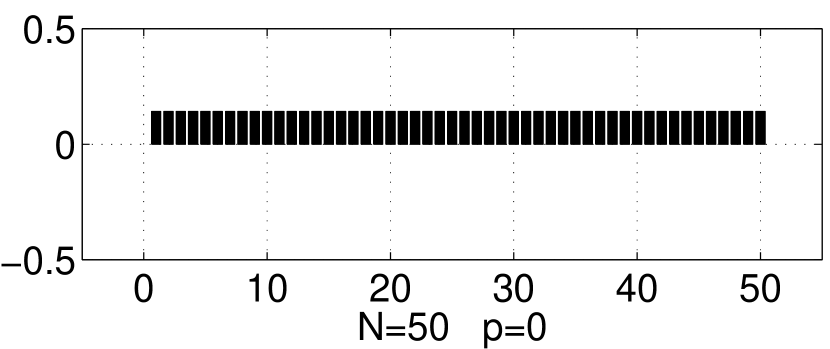
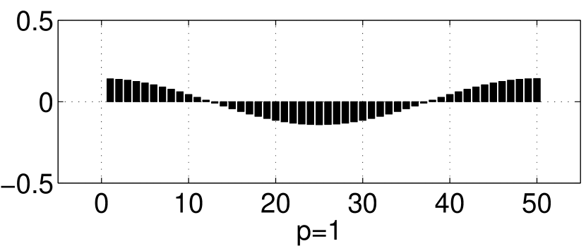
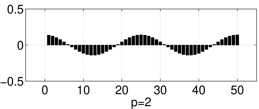
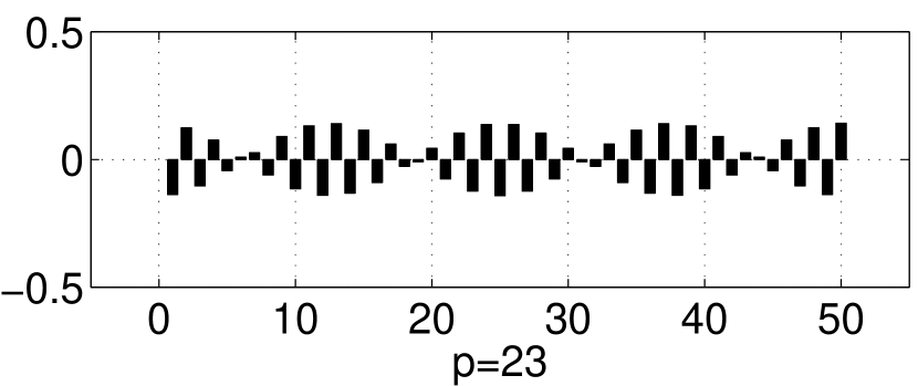
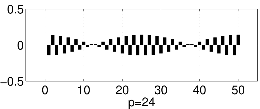
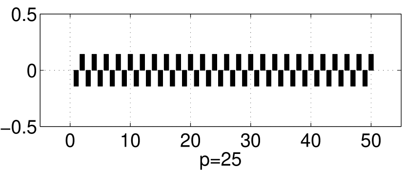
Figure 3: The real parts $\mathfrak{Re}\!~{}c^{p}_{A}$ of the components of states (24a, 23) in the uncorrelated basis, for the eigenstates $p=0,1,2,23,24,25$ of a configuration with $N=50$ outer atoms. For $p\neq 0$ these coefficients are the same for both configurations (a) and (b).

If $p=0$, the associated eigenspace $\mathsf{T}_{0}$ is one-dimensional for configuration (b), and is spanned by

$$\left|\mathcal{C}_{0}\right\rangle\equiv\frac{1}{\sqrt{N}}\sum_{A=1}^{N}\left|A,0\right\rangle\quad,$$ (24a)

while, for configuration (a), $$\mathsf{T}_{0}$$ is two-dimensional, with a second basis vector

$$\left|\mathcal{C}_{z}\right\rangle\equiv\left|z,0\right\rangle\quad.$$ (24b)

The two states in (24) are totally isotropic under the symmetry group $\mathbb{Z}_{N}$ in the sense that they do not pick up a phase factor when we operate with a group element on them. Furthermore, they are “extreme” states, since in (24a), only outer atoms are occupied, with all atomic dipoles aligned parallely, as can be seen in the first plot in Fig. 3; while in (24b), only the central atom is occupied.

V Diagonalization of the channel Hamiltonian on carrier spaces of the symmetry group

V.1 Configuration (b)

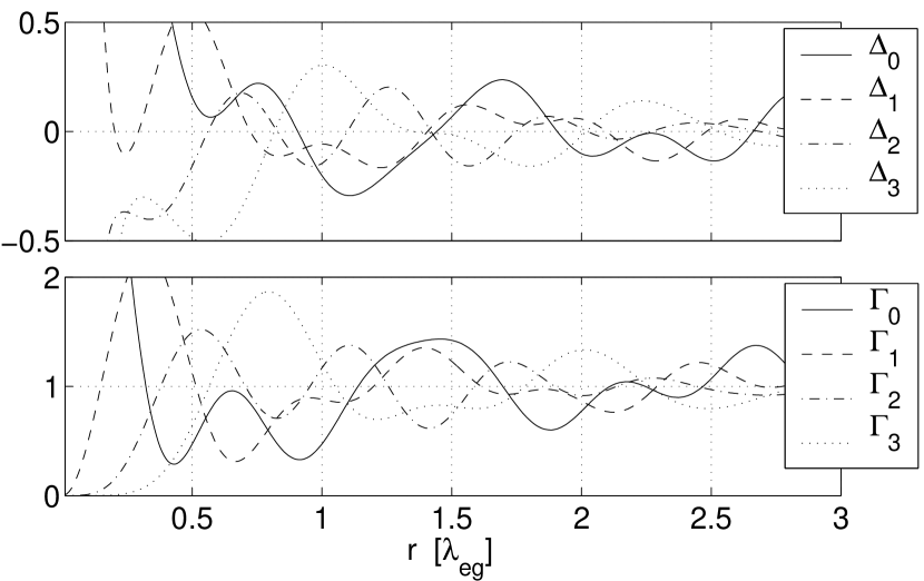
Figure 4: Relative level shifts $\widetilde{\Delta}_{p}/\Gamma$ and decay rates $\Gamma_{p}/\Gamma$ for the states $p=0,1,2,3$ with $N=7$ outer atoms and no central atom. From the second plot we see that none of the $p$-states can generally be declared as super- or subradiant; rather, for each state there exist ranges of the radius $r$ for which the state $\left|\mathcal{C}_{p}\right\rangle$ is maximally super- or maximally subradiant. The physical reason for this dependence lies in the interference due to varying phase differences between spatially retarded radiative contributions from all but one atom, at the site of the given atom.

We first discuss configuration (b) without central atom. In this case, each of the carrier spaces $\mathsf{T}_{p}$ is one-dimensional, and is spanned by states (23, 24a). Since $\mathcal{H}$ and $\mathcal{R}$ preserve these carrier spaces it follows that each of the $\left|\mathcal{C}_{p}\right\rangle$, $p=0,\ldots,N-1$ is automatically a right eigenvector of $\mathcal{R}$, with eigenvalue

$$\mu_{p} =-\frac{2\widetilde{\Delta}_{p}}{\Gamma}+i\frac{\Gamma_{p}}{\Gamma}\quad,$$ (25a)

$$\widetilde{\Delta}_{p} =-\frac{\Gamma}{2}\sum_{A=2}^{N}S(k_{eg}R_{1A})\,\cos\left(\frac{2\pi p(A-1)}{N}\right)\quad,$$ (25b)

$$\Gamma_{p} =\Gamma\Bigg{\{}1+\sum_{A=2}^{N}D_{1}(k_{eg}R_{1A})\,\cos\left(\frac{2\pi p(A-1)}{N}\right)\Bigg{\}}\quad,$$ (25c)

where we have used (40). It follows that

$$\mu_{N-p}=\mu_{p}\quad,$$ (26)

hence some of the eigenvalues are degenerate; the exact result is presented in Table 1. Eqs. (25b) and (25c) contain the level shifts and decay rates, which are given as cosine transformations of the correlation functions $S$ and $D_{1}$. A plot of these quantities for the first four eigenvalues for $N=7$ outer atoms is given in Fig. 4, where the approximated shift function $S_{\text{approx}}$ based on eq. (7) has been used.

V.2 Mechanisms for super- and subradiance

The Figures 3 and 4 give some insight into the mechanism of super- and subradiance. We first note that the system atoms+radiation evolves unitarily in the present treatment, and since the initial state was pure, the state of the total system is always pure. This fact entitles us to visualize the atoms in the sample as being radiating coherently. This coherence is at the heart of super- and subradiance since it means that the radiative contributions emitted by the individual atoms will interfere: generally speaking, a correlated state will be super- or subradiant when the total interference between these contributions is constructive or destructive in the far zone (measured in units of $\lambda_{eg}$) of the radiation field around the configuration. Based on this reasoning we now give a qualitative explanation for the behaviour of level shifts and decay rates in Fig. 4 in the small-sample limit $r\rightarrow 0$:

Level degeneracy for configurations (a) and (b)

$$\begin{array}[]{| @{\hspace{.5em}} r @{\hspace{.5em}} || @{\hspace{.5em}} r@{}c@{}l @{\hspace{.1em}} @{\hspace{.5em}} | @{\hspace{.5em}} r@{}c@{}l @{\hspace{.5em}} |}\hline\cr\hskip 5.0pt\lx@intercol\hfil\hskip 5.0pt\vrule\vrule\hskip 5.0pt&N&=&2n+1\hfil\hskip 1.00006pt\hskip 5.0pt\vrule\hskip 5.0pt&N&=&2n\hfil\hskip 5.0pt\\ \hline\cr\hline\cr\hskip 5.0pt\lx@intercol\hfil\text{degenerate}\hskip 5.0pt\vrule\vrule\hskip 5.0pt&p&=&\begin{array}[]{r@{}c@{}l}1,&\ldots,&n\\ 2n,&\ldots,&n+1\end{array}\hfil\hskip 1.00006pt\hskip 5.0pt\vrule\hskip 5.0pt&p&=&\begin{array}[]{r@{}c@{}l}1,&\ldots,&n-1\\ 2n-1,&\ldots,&n+1\end{array}\hfil\hskip 5.0pt\\ \hline\cr\hskip 5.0pt\lx@intercol\hfil\text{non-degenerate}\hskip 5.0pt\vrule\vrule\hskip 5.0pt&p&=&0\,(\pm)\hfil\hskip 1.00006pt\hskip 5.0pt\vrule\hskip 5.0pt&p&=&0\,(\pm),n\hfil\hskip 5.0pt\\ \hline\cr\end{array}$$

Table 1: Degeneracy of the eigenvalues for quantum numbers $p=0(\pm),\ldots,N-1$, for odd and even $N$, for configurations (a) and (b). Vertically stacked $p$ values in the second row are mutually degenerate.

We see in Fig. 4 that the $p=0$ state is the only one which has a nonvanishing decay rate in this limit: All atomic dipoles are aligned parallely in this state [see eq. (24a) and first plot in Fig. 3], and vanishing interatomic distance on a length scale of a wavelength means that the radiation emitted coherently by the sample must interfere completely constructively. Hence, the sample radiates faster than a single atom by a factor $N$, since the decay rate is

$$\lim\limits_{r\rightarrow 0}\Gamma_{p=0}=N\cdot\Gamma\quad,$$ (27)

as follows from eq. (25). Conversely, the suppression of spontaneous decay for the states with $p>0$ is a consequence of the fact that the dipoles have alternating orientations, see eq. (23) and the second to fifth plot in Fig. 3, so that, in the small-sample limit $r\rightarrow 0$, roughly one-half of the atoms radiate in phase, while the other half has a phase difference of $\pi$; hence

$$\lim\limits_{r\rightarrow 0}\Gamma_{p>0}=0\quad.$$ (28)

This behaviour is exemplified by the plots of $\Gamma_{1},\Gamma_{2},\Gamma_{3}$ in Fig. 4. However, the destructive interference in the $(p>0)$ states is independent of how adjacent dipoles are oriented, as long as $r\ll\lambda_{eg}$; in this limit, the decay rate should not be noticeably affected by rearranging the dipoles in different patterns as long as the 50:50 ratio of parallel-antiparallel dipoles is kept fixed. What will be affected by such a redistribution is the level shift, since the Coulomb interaction between the dipoles in the sample may change towards more attraction or repulsion between the atoms. By this mechanism we can explain the divergent behaviour of the level shifts in the small-sample limit: The shift of the $p=0$ state always behaves like

$$\lim\limits_{r\rightarrow 0}\Delta_{p=0}=+\infty\quad,$$ (29)

which arises from the Coulomb repulsion of the parallely aligned dipoles. On the other hand, the level shifts for the $(p>0)$ states depend on the relative number of parallely aligned dipoles in the immediate neighbourhood of a given dipole, or conversely, on the degree of balancing the Coulomb repulsion by optimal pairing of antiparallel dipoles. As a consequence, states for which $p$ is close to zero always have positive level shifts, since the Coulomb interaction between adjacent dipoles tends to be repulsive, as seen in the first three plots in Fig. 3, and the behaviour of $\Delta_{0},\Delta_{1}$ in Fig. 4. On the other hand, states for which $p$ is close to $N/2$ tend to have antiparallel orientation between adjacent dipoles, hence the Coulomb interaction is now largely attractive, which explains why these states have negative level shifts in the limit $r\ll\lambda$. This is seen in the last three plots in Fig. 3 and the behaviour of $\Delta_{2},\Delta_{3}$ in Fig. 4.

The same mechanism clearly also governs the super- or subradiance of the sample with finite interatomic distance. In this case the information about the orientation of surrounding dipoles at sites $\mathbf{R}_{A}$ is contained in the transverse electric field, which arrives at the site $\mathbf{R}_{1}$ with a retardation $|\mathbf{R}_{A}-\mathbf{R}_{1}|/c$. Thus, in addition to the phase difference imparted by the coefficients $c^{p}_{A}$, there is another contribution to the phase from the spatial retardation, which accounts for the dependence of the level shifts and decay rates on the radius $r$. However, apart from this additional complication, the physical mechanism determining whether a given state is super- or subradiant is clearly the same as in the small-sample limit, and can be traced back to the mutual interference of the radiation emitted by each atom, arriving at a given site $\mathbf{R}_{1}$.

V.3 Configuration (a)

Now we turn to compute the complex energy eigenvalues and eigenvectors for configuration (a) with central atom. For $p=1,\ldots,N-1$, the basis vectors carrying irreducible representations of the symmetry group are the same as before, and are given in eq. (23). Consequently, they are also right eigenvectors of the matrix $\mathcal{R}$; the associated eigenvalues $\mu_{p}$ turn out to be the same as for configuration (b) and thus are given by formulas (25). This result means that the presence or absence of the central atom is not “felt” by the system in the modes $\left|\mathcal{C}_{p}\right\rangle$, $p=1,\ldots,N-1$, since the central atom is not occupied in these states.

On the other hand, the eigenspace $\mathsf{T}_{0}$ of $T$ corresponding to the $p=0$ representation is now two-dimensional and is spanned by $\Gamma^{0}$-basis vectors (24a) and (24b). We now need to diagonalize the channel Hamiltonian on this subspace: the diagonalization of the matrix $\mathcal{R}$ in the basis $\left|\mathcal{C}_{0}\right\rangle,\left|\mathcal{C}_{z}\right\rangle$ yields

$$\left|\mathcal{C}_{0+}\right\rangle =\hskip 2.15277pt\cos\widehat{\theta}\,\left|\mathcal{C}_{0}\right\rangle+\sin\widehat{\theta}\,\left|\mathcal{C}_{z}\right\rangle\quad,$$ (30a)

$$\left|\mathcal{C}_{0-}\right\rangle =-\sin\widehat{\theta}\,\left|\mathcal{C}_{0}\right\rangle+\cos\widehat{\theta}\,\left|\mathcal{C}_{z}\right\rangle\quad,$$ (30b)

where

$$\widehat{\theta}=\frac{i}{2}\ln\frac{i+c}{i-c}\quad,$$ (31)

with

$$c=\frac{2\sqrt{N}\,M(k_{eg}r)}{\sum_{A=2}^{N}M(k_{eg}R_{1A})+\sqrt{\left[\sum_{A=2}^{N}M(k_{eg}R_{1A})\right]^{2}+4N\,M^{2}(k_{eg}r)}},$$ (32)

and $M=S+iD_{1}$. The eigenvectors (30) are not orthogonal, consistent with the fact that the matrix $\mathcal{R}$ is not Hermitean. However, (30) form an orthonormal system together with the left eigenvectors

$$\left\langle\mathcal{C}_{0+}^{*}\right| =\hskip 2.15277pt\cos\widehat{\theta}\,\left\langle\mathcal{C}_{0}\right|+\sin\widehat{\theta}\,\left\langle\mathcal{C}_{z}\right|\quad,$$ (33)

$$\left\langle\mathcal{C}_{0-}^{*}\right| =-\sin\widehat{\theta}\,\left\langle\mathcal{C}_{0}\right|+\cos\widehat{\theta}\,\left\langle\mathcal{C}_{z}\right|\quad.$$

The associated eigenvalues $\mu_{0\pm}$ (of $\mathcal{R}$) are

$$\mu_{0\pm} =i+\frac{1}{2}\sum_{A=2}^{N}M\left(k_{eg}R_{1A}\right)\pm$$ (34)

$$\pm\frac{1}{2}\sqrt{\left[\sum_{A=2}^{N}M\left(k_{eg}R_{1A}\right)\right]^{2}+4N\,M^{2}\left(k_{eg}r\right)}\quad,$$

where $r$ is the radius of the circle. From (34) we obtain the level shifts $\widetilde{\Delta}_{0\pm}$ and decay rates $\Gamma_{0\pm}$ of the $p=0$ states as in eq. (25).

The definition of eigenvalues $\mu_{0\pm}$ as given in eq. (34) is not yet the final one, however. In (34) we have assigned $\mu_{0+}$ to the square root with positive real part. From (14a) we see that the $\mu_{0+}$ so defined always comes with a negative level shift, and therefore the associated real energy $\widetilde{E}_{i}+\hbar\widetilde{\Delta}_{0+}$ is always smaller than the energy associated with $\mu_{0-}$. This state of affairs would be acceptable as long as the levels would never cross; but crossing they do, as can be seen in Fig. 5:

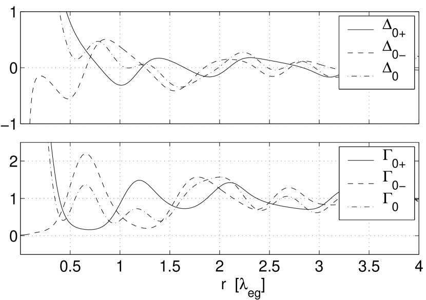
Figure 5: Plotted are relative quantities $\widetilde{\Delta}_{0(\pm)}/\Gamma$ and $\Gamma_{0(\pm)}/\Gamma$. For $N=10$ outer atoms, the level shifts $\widetilde{\Delta}_{0\pm}$ exhibit level crossing twice on every wavelength, for $r\geq\lambda_{eg}$. At the radius $r$ of a crossing, the beat frequency (37) vanishes, preventing any oscillatory population transfer between $\left|\mathcal{C}_{0}\right\rangle$ and $\left|\mathcal{C}_{z}\right\rangle$. The states $\left|\mathcal{C}_{0\pm}\right\rangle$ are defined such that, as $r\rightarrow 0$, the level shifts $\widetilde{\Delta}_{0\pm}$ tend to $\pm\infty$, respectively. — For comparison, level shifts and decay rates of the state $\left|\mathcal{C}_{0}\right\rangle$ without central atom are included.

For radii greater than a certain lower bound $r_{0}$, which depends on the number $N$ of outer atoms, we see two level-crossings per unit wavelength. For $N=10$ this radius is roughly $r_{0}\sim\lambda$. At each crossing we have to reverse the assignment of square roots to eigenvalues in order to obtain smooth eigenvalues. We therefore have to redefine $\mu_{0\pm}$, and the associated eigenvectors, in order to take account of this reversal. A look at Fig. 5 shows that, for $r\leq 0.7~{}\lambda$, no crossings occur, so that we can uniquely identify the eigenvalues by their behaviour in the limit $r\rightarrow 0$. Thus, we finally define $\mu_{0\pm}$ to be that eigenvalue whose associated level shift $\widetilde{\Delta}_{0\pm}=-\Gamma\mathfrak{Re}\!~{}\mu_{0\pm}/2$ tends towards $\pm\infty$, respectively. Physically, the dipoles in the state $\left|\mathcal{C}_{0+}\right\rangle/\left\|\mathcal{C}_{0+}\right\|$ are aligned parallely, which in the limit $r\rightarrow 0$ produces Coulomb repulsion, and hence the positive level shift. It follows that the state $(p=0+)$ is the natural analogue of the $(p=0)$ state in configuration (b), since they both have the same behaviour at small radii. It is also expected to decay much faster than a single atom, an expectation which is confirmed by the behaviour of the imaginary part $\mathfrak{Im}\!~{}\mu_{0+}=\Gamma_{0+}/\Gamma$, which tends to $\sim N+1$ as $r\rightarrow 0$. Again this follows the pattern of the $p=0$ state in configuration (b). A visual comparison between states $(p=0+)$ and $(p=0)$ is given in Fig. 5 for $N=10$ outer atoms.

On the other hand, in the state $\left|\mathcal{C}_{0-}\right\rangle/\left\|\mathcal{C}_{0-}\right\|$, the central atom is now oriented antiparallelly to the common orientation of the outer dipoles, and, in the limit $r\rightarrow 0$, is much stronger occupied than the outer atoms, as follows from eq. (30b). Hence, as a consequence of Coulomb attraction between the outer atoms and the central atom, the energy is shifted towards $-\infty$, and at the same time, the system has become extremely stable against spontaneous decay: This is reflected in the fact that, as $r\rightarrow 0$, the decay rate $\Gamma_{0-}$ tends to zero as well.

As mentioned above, the states with higher quantum numbers $p=1,\ldots,N-1$ are the same as in configuration (b), and have the same eigenvalues. The two levels $p=(0\pm)$ are non-degenerate, except for accidental degeneracy, and also are non-degenerate with the $(p>0)$ levels. As a consequence, the level degeneracy is similar to case (b), and is again expressed in Table 1.

V.4 Quantum beat between unperturbed $p=0$ states

As follows from eqs. (30), the true eigenstates $\left|\mathcal{C}_{0\pm}\right\rangle$ are in general linear combinations of the ”unperturbed” irreducible basis vectors $\left|\mathcal{C}_{0}\right\rangle$, eq. (24a), and $\left|\mathcal{C}_{z}\right\rangle$, eq. (24b); as a consequence, the true eigenstates will give rise to a quantum beat between $\left|\mathcal{C}_{0}\right\rangle$ and $\left|\mathcal{C}_{z}\right\rangle$. In order to determine the beat frequency we compute the probability of finding the system at time $t$ in the extreme state $\left|\mathcal{C}_{0}\right\rangle$ if initially it was in the other extreme state $\left|\mathcal{C}_{z}\right\rangle$,

$$P_{\left|\mathcal{C}_{z}\right\rangle\rightarrow\left|\mathcal{C}_{0}\right\rangle}(t) =\Big{|}\left\langle\mathcal{C}_{0}\right|U(t,0)\left|\mathcal{C}_{z}\right\rangle\Big{|}^{2}=\left|\sin\widehat{\theta}\cos\widehat{\theta}\right|^{2}\,\times$$

$$\times\,\Bigg{\{}e^{-\Gamma_{0+}t}+e^{-\Gamma_{0-}t}-2\,e^{-\frac{1}{2}\left(\Gamma_{0+}+\Gamma_{0-}\right)t}\times$$

$$\times\cos\left[\left(\widetilde{\Delta}_{0+}-\widetilde{\Delta}_{0-}\right)t\right]\Bigg{\}}\quad.$$ (35)

The last line shows that the oscillation between the two states occurs at the beat frequency

$$\omega_{R}=\left|\widetilde{\Delta}_{0+}-\widetilde{\Delta}_{0-}\right|\quad.$$ (36)

The beat frequency can be expressed in terms of the function $M=S+iD_{1}$ as

$$\omega_{R}=\frac{\Gamma}{2}\mathfrak{Re}\!~{}\sqrt{\left[\sum_{A=2}^{N}M\left(k_{eg}R_{1A}\right)\right]^{2}+4N\,M^{2}\left(k_{eg}r\right)}\quad.$$ (37)

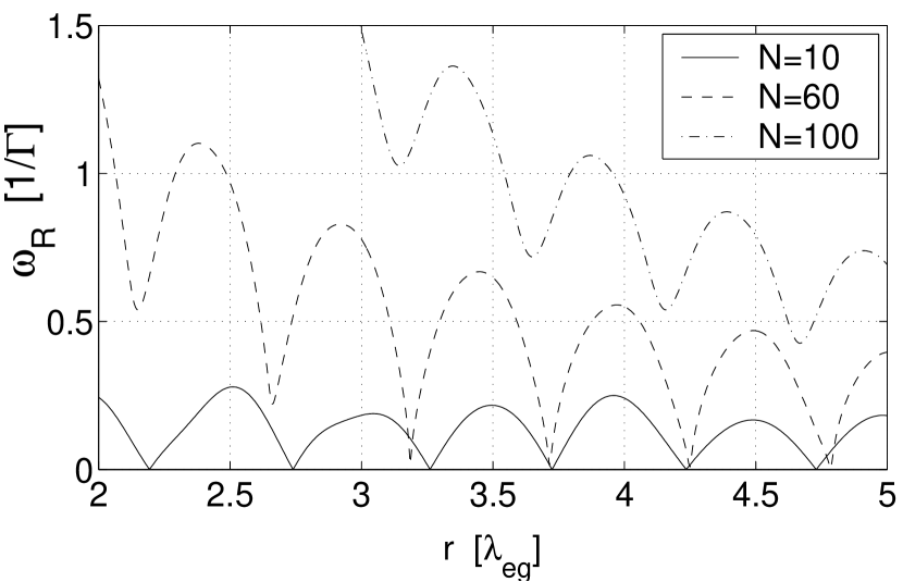
Figure 6: The beat frequency eq. (37) for three different values $N=10,60,100$ of outer atoms, for radii between $2$ and $5$ wavelengths. At the radius of a level crossing $\widetilde{\Delta}_{0+}=\widetilde{\Delta}_{0-}$, the beat frequency vanishes. It can be seen that the greater the number of outer atoms $N$, the greater becomes the radius $r_{0}$ beyond which level crossing occurs.

For a given number of outer atoms, there can exist discrete radii at which the beat frequency $\omega_{R}$ vanishes. From formula (36) we see that this is the case precisely when the two levels cross, and hence the normalized states $\left|\mathcal{C}_{0+}\right\rangle$ and $\left|\mathcal{C}_{0,-}\right\rangle$ are degenerate in energy. This is demonstrated in Fig. 6.

The beat frequency $\omega_{R}$ so computed has to be treated with a grain of salt, however. The reason is that the dynamics in the radiationless $Q$-space does not preserve probability flux, since the latter decays into the $P$-space when occupying the modes of outgoing photons. This is reflected in the presence of damped exponentials in formula (35). Depending on the number of atoms involved and the radius of the circle, this damping may be so strong, compared to the amplitude of the beat oscillations, that the dynamical behaviour effectively becomes aperiodic, i.e., exhibits no discernable oscillations. An example is given by the $N=10$ plot in Figure 7.

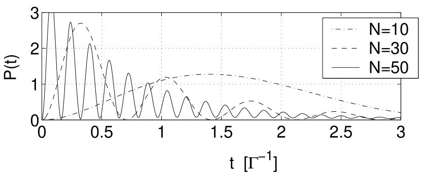
Figure 7: The probability $P(t)/|\sin\widehat{\theta}\cos\widehat{\theta}|^{2}$ for the transition $\left|\mathcal{C}_{z}\right\rangle\rightarrow\left|\mathcal{C}_{0}\right\rangle$, as given in eq. (35), for $N=10,30,50$ outer atoms, at a radius $r=0.45~{}\lambda_{eg}$. The beat oscillations for $N=10$ are practically invisible, making the transfer effectively aperiodic.

V.5 Analogy between $p=0$ states and hydrogen-like $s$ states

It is interesting to note that for the $p\neq 0$ states, the central atom is unoccupied, irrespective of the radius of the circle, or the number of atoms in the configuration. This means that the central atom takes part in the dynamics only in a $p=0$ state. This is strongly reminiscent of the behaviour of scalar single-particle wavefunctions in a Coulomb potential, such as a spinless electron in a hydrogen atom: In this case, the electronic wavefunction vanishes at the origin of the coordinate system, i.e., at the center-of-symmetry of the potential, for all states with orbital angular momentum quantum number $l$ greater than zero. On the other hand, in the case of our planar atomic system, the circular configurations also have a center-of-symmetry, namely the center of the circle. We can interpret the “Frenkel excitons” $\left|\mathcal{C}_{p}\right\rangle/\left\|\mathcal{C}_{p}\right\|$ as states of a single quasi-particle, which is distributed over the set of discrete locations $\mathbf{R}_{z},\mathbf{R}_{A}$ corresponding to the sites of the atoms. Then the amplitudes $\left\langle A,0|\mathcal{C}_{p}\right\rangle=c^{p}_{A}$ play a role analogous to a spatial wavefunction $\left\langle\mathbf{x}|\psi\right\rangle=\psi(\mathbf{x})$; and just as the hydrogen-like wavefunctions vanish at the origin for angular momentum quantum numbers $l\neq 0$ Bransden and Joachain (2003), so vanish our quasi-particle wavefunctions at the central atom for all quantum numbers other than $p=0$. In both cases, the associated wave functions are isotropic: The $s$-states transform under the identity representation ($l=0$) of $SO(3)$ in the case of hydrogen-like systems, and states $\left|\mathcal{C}_{0(\pm)}\right\rangle$ under the identity representation $(p=0)$ of $\mathbb{Z}_{N}$ in the case of our circular configurations. This means that the quantum number $p$ is analogous to the angular momentum quantum number $l$ in the central-potential problem; with hindsight, this may not surprising, since both quantum numbers $p$ and $l$ are indices which label the unitary irreducible representations of rotational symmetry groups $\mathbb{Z}_{N}$ and $SO(3)$.

VI Photon trapping in maximally subradiant states

In this section we are interested in the photon-trapping capability of maximally subradiant states, for large numbers of atoms in the circle. To this end we choose a fixed radius, increase the number of atoms in the configuration gradually, and, for each number $N$, compute the decay rate $\Gamma_{{\text{min}}}$ of the maximally subradiant state for the given pair $(r,N)$, in configuration (b) only. We then expect a more or less monotonic decrease of $\Gamma_{\text{min}}$ as $N$ increases. But what precisely is the law governing this decrease? A numerical investigation gives the following result: In Fig. 8 we plot the negative logarithm $-\ln(\Gamma_{\text{min}}/\Gamma)$ of the minimal relative decay rate at the radii $r=1,1.5,2,2.5~{}\lambda$ for increasing numbers of atoms. We see that from a certain number $N=\hat{N}$ onwards, which depends on the radius, $-\ln(\Gamma_{\text{min}}/\Gamma)$ increases approximately linearly with $N$; in the figure, we have roughly $\hat{N}=14$ for $r=\lambda$, $\hat{N}=20$ for $r=1.5~{}\lambda$, $\hat{N}=26$ for $r=2~{}\lambda$, $\hat{N}=33$ for $r=2.5~{}\lambda$. We also see that the slope is a function of the radius $r$.

We note that the four curves in Fig. 8 imply the existence of a common critical interatomic distance: For large $N$, the next-neighbour distance $R_{nn}$ between two atoms on the perimeter of the circle is roughly equal to $2\pi r/N$; if we compute this distance for the pairs of values $(r,\hat{N})$ as found above we obtain $R_{nn}=0.45,0.47,0.48,0.48~{}\lambda$, respectively. We see that a critical next-neighbour distance of $R_{c}\approx 0.5~{}\lambda$ presents itself: If, for fixed radius $r$, the number of atoms in the configuration is increased, the next-neighbour distance $R_{nn}$ decreases; as soon as $R_{nn}=R_{c}$ is reached, the order of magnitude by which spontaneous emission from the maximally subradiant state is suppressed becomes approximately proportional to $N$.

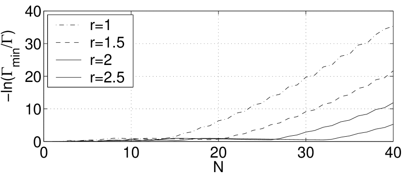
Figure 8: The negative logarithm of the minimal relative decay rate, being proportional to the order of magnitude of suppression of spontaneous decay, as a function of the number of atoms $N$, for fixed radii as given in the legend. We see that for each radius there exists a critical number $\hat{N}$ of atoms in the configuration beyond which the order of magnitude by which spontaneous emission is suppressed is roughly proportional to $N$. In the Figure, these critical values are roughly at $\hat{N}=14,20,26,33$ atoms. Beyond these values, the next-neighbour distance, which is roughly equal to $2\pi r/N$, becomes smaller than the critical distance $\lambda_{eg}/2$.

Based upon this reasoning we see that, for a given radius $r$, the critical number $\hat{N}$ of atoms in configuration (b) is given by $\hat{N}=\frac{4\pi r}{\lambda}$. Then, we infer from Fig. 8 that, approximately,

$$\Gamma_{\text{min}}\simeq\Gamma\cdot e^{-s(r)(N-\hat{N})}\quad,\quad\text{for $N>\hat{N}$}\quad,$$ (38)

where $s(r)$ determines the slopes of the curves in Fig. 8; this function decreases monotonically with $r$. We must have the limit $s(r)\xrightarrow{r\rightarrow\infty}0$, because for large radii all correlations between atoms must cease to exist, and hence $\Gamma_{\text{min}}\rightarrow\Gamma$ in this limit. Let $\tau\equiv 1/\Gamma$ denote the lifetime of the excited level in a single two-level atom; then formula (38) tells us that the lifetime $\tau_{\text{min}}$ of a maximally subradiant state pertaining to $\Gamma_{\text{min}}$ increases exponentially with the number of atoms,

$$\tau_{{\text{min}}}=\tau\cdot e^{s(r)(N-\hat{N})}\quad,\quad\text{for $N>\hat{N}$}\quad.$$ (39)

Theoretically, at least, we can therefore keep a photon trapped in a circular configuration for arbitrarily large lifetimes, just by increasing the number of atoms in the circle, hence decreasing the next-neighbour distance. In practice, of course, a lower limit would be attained when the wavefunctions of adjacent atoms start to overlap. Furthermore, the impact of the environment on the coherence of the maximally subradiant state must be taken into account:

VII Dephasing: the impact of an environment

The results presented so far have been idealized in that it was assumed that the system was closed, being protected from random noise and loss of quantum coherence into the environment and thus evolving unitarily. In practice, of course, this cannot be the case any longer. Through interactions and subsequent entanglement with an environment, the subsystem atoms+radiation will loose the purity of the initial state, which will turn into a mixture. This loss is associated with the intrusion of random elements into the evolution of the subsystem, of which two generic types may be conceptualized:

Firstly, the sites $\mathbf{R}_{A},\mathbf{R}_{z}$ of the atomic dipoles will undergo random fluctuations at finite temperature; these fluctuations will impart small random phases on the radiative contributions emitted from the individual atoms in the configuration, so that the radiation from the sample will no longer be completely coherent. This reduction in coherence will reduce both the super- and the subradiance of collective states, since it is the interference based on coherence which is responsible for these effects. We therefore expect that the radiative decay rates of the superradiant states become smaller, while those of the subradiant states will increase. Nevertheless, this effect may be expected to be small, since the amplitudes of oscillations of the atomic sites will be on the order of a Bohr radius, while, in the present scenario, the wavelengths of the electronic transitions are in the optical regime.

Secondly, quantum coherence of the subsystem atoms+radiation will be reduced by phonon-induced or collisionally-induced dephasing in the phases of the quantum states, produced by small random shifts in the unperturbed ground- and excited-state energies of the single atoms due to the coupling to the environment. It is possible to take these random elements into account phenomenologically by averaging over the acquired random phase shifts; in the limit of infinitely short memory (Markoff approximation) we then arrive at a dephasing-decay rate which must be added to the radiative decay rate Meystre and III (1998).

In such a case the evolution of the subsystem atoms+radiation must be described by an appropriate master equation for the associated reduced density operator. For example, in a solution, the typical nonradiative decay channel will be comprised of conversions of the exciton energy into thermal vibrational energy, in other words, a transition from the electronic excitation into a large number of phonons. The phase of the coherent, wavelike motion of the exciton, as exemplified in Fig. 3, then decays on account of the interaction with intra- and intermolecular vibrations. These vibrations, in turn, give rise to fluctuations of the excitation energies and of the interaction matrix elements and must be taken into account in the Hamiltonian by an additional, stochastically time-dependent contribution. Averaging the equation of motion of the density operator over the fluctuations results in the stochastic Liouville equation describing the exciton dynamics Kubo (1963); Haken and Strobl (1967); Haken and Reineker (1972); Haken and Strobl (1973); Aslangul and Kottis (1974); Reineker (1979); Aslangul and Kottis (1980). The phonons can also be treated as a quantum-mechanical heat bath Haken and Reineker (1968); Weidlich and Haake (1965a, b); Haake (1973).

In each case additional, nonradiative decay channels open up, with associated decay rates. Only when these decay rates are small compared to the idealized radiative decay rates studied in this work will the results obtained here continue to make sense. We hope to be able to come back to this point in the future.

VIII Summary

Collective excitations together with associated level shifts and decay rates in a planar circular configuration of identical two-level atoms with parallel atomic dipoles are examined. The relation between these states to traditional Frenkel excitons is discussed. The state space of the atomic system can be decomposed into carrier spaces pertaining to the various irreducible representations of the symmetry group $\mathbb{Z}_{N}$ of the system. Accordingly, the channel Hamiltonian on the radiationless subspace of the system can be diagonalized on each carrier space separately, making an analytic computation of eigenvectors and eigenvalues feasable. Each eigenvector can be uniquely labelled by the index $p$ of the associated representation. For quantum numbers $p>0$ the circular configuration is insensitive to the presence or absence of a central atom, so that the wavefunction of the associated quasi-particle describing the collective excitation occupies the central atom only in a $p=0$ state. It is explained how this feature is analogous to the behaviour of hydrogen-like $s$-states in a Coulomb potential. The presence of a central atom causes level splitting and -crossing of the $p=0$ state, in which case damped oscillations between two ”extreme” $p=0$ configurations occur. For strong damping, the population transfer between the two extreme configurations is effectively aperiodic. Finally, the behaviour of the minimal decay rate in maximally subradiant states for varying numbers of atoms in the configuration is investigated; a critical number of atoms, corresponding to a next-neighbour distance of $\lambda_{eg}/2$ on the circle, exists, beyond which the lifetime of the maximally subradiant state increases exponentially with the number of atoms in the configuration.

IX Appendix

Here we prove a technical result which is used in the main part of the paper:

Let $R_{1A}$ denote the distance between atoms $1$ and $A$ (i.e., outer atoms only). Let $F$ be any function of this distance, $F=F(R_{1A})$. Let $p$ be an integer. Then

$$\sum_{A=2}^{N}F(R_{1A})\,\sin\left(\frac{2\pi p}{N}(A-1)\right)=0\quad.$$ (40)

Proof:

The sum $S$ can be written as

$$S=\sum_{A=2}^{N}F(R_{1,N-A+2})\,\sin\left(\frac{2\pi p}{N}(N-A+1)\right)\quad.$$ (41)

The sines are equal to

$$\sin\left(\frac{2\pi p}{N}(N-A+1)\right)=-\sin\left(\frac{2\pi p}{N}(A-1)\right)\quad,$$ (42)

while the distances satisfy the equations

$$R_{1,N-A+2}=R_{1A}\quad.$$ (43)

If this is inserted into (41) we obtain an expression which is the negative of (40), and as a consequence, $S$ must be zero. $\blacksquare$