Resilience of multi-photon entanglement under losses

Abstract

We analyze the resilience under photon loss of the bi-partite entanglement present in multi-photon states produced by parametric down-conversion. The quantification of the entanglement is made possible by a symmetry of the states that persists even under polarization-independent losses. We examine the approach of the states to the set of states with a positive partial transpose as losses increase, and calculate the relative entropy of entanglement. We find that some bi-partite distillable entanglement persists for arbitrarily high losses.

I Introduction

Parametric down-conversion has been used in many experiments pdcexp to create polarization entangled photon pairs kwiat . Recent experimental lamasdemart ; eisenberg and theoretical durkin ; simon ; reid work has studied the creation of strong entanglement of large numbers of photons. The states under consideration are entangled pairs of light pulses such that the polarization of each pulse is completely undetermined, but the polarizations of the two pulses are always anti-correlated. Such states are the polarization equivalent of approximate singlet states of two potentially very large spins howell . An application of the states for quantum key distribution has been suggested durkin .

In any realistic experiment photons will be lost during propagation. It is therefore of great practical interest to analyze the resilience of the multi-photon entanglement under loss. A priori this seems like a very difficult task, because it requires the quantification of the entanglement present in mixed quantum states of high or actually even infinite dimensionality. However, the multi-photon states introduced in the above work exhibit very high symmetry - in the absence of losses they are spin singlets. The related symmetry under joint polarization transformations on both pulses is preserved even in the presence of polarization-independent losses. This makes it possible to apply the concepts of ‘entanglement under symmetry’ developed in Refs. Werner ; Rains ; Sym ; Regul ; KGH to the quantification of the multi-photon entanglement in the presence of losses. We calculate the degree of entanglement for the resulting states of high symmetry, as quantified in terms of the relative entropy of entanglement. We show that some (distillable) entanglement remains for arbitrarily high losses.

II Symmetry of the states in the presence of losses

In the above-mentioned experiments and proposals a non-linear crystal is pumped with a strong laser pulse, and a three-wave mixing effect leads to the creation of photons along two directions $a$ and $b$. To a good approximation the Hamiltonian in the interaction picture in a four-mode description is given by

$$H=e^{i\phi}\kappa({a}_{h}^{\dagger}{b}_{v}^{\dagger}-{a}_{v}^{\dagger}{b}_{h}^{\dagger})+e^{-i\phi}\kappa({a}_{h}{b}_{v}-{a}_{v}{b}_{h}).$$ (1)

The real coupling constant $\kappa$ is proportional to the amplitude of the pump field and to the relevant non-linear optical coefficient of the crystal, and $\phi$ denotes the phase of the pump field. Photons are created into the four modes with annihilation operators $a_{h}$, $a_{v}$, $b_{h}$, $b_{v}$, where $h$ and $v$ denote horizontal and vertical polarization. Note that both the modes and the associated annihilation operators will be denoted with the same symbol. In the absence of losses, this Hamiltonian leads to a state vector of the form durkin ; simon

$$|\psi\rangle=e^{-iHt}|0\rangle=\frac{1}{\cosh^{2}\tau}\sum_{n=0}^{\infty}e^{in\phi}\sqrt{n+1}\;\tanh^{n}\tau\;|\psi^{n}_{-}\rangle,$$ (2)

where $\tau=\kappa t$ is the effective interaction time and

$$|\psi^{n}_{-}\rangle=\frac{1}{\sqrt{n+1}}\frac{1}{n!}(a^{\dagger}_{h}b^{\dagger}_{v}-a^{\dagger}_{v}b^{\dagger}_{h})^{n}|0\rangle$$ (3)

$$=\frac{1}{\sqrt{n+1}}\sum_{m=0}^{n}(-1)^{m}|n\!\!-\!\!m\rangle_{a_{h}}|\,m\rangle_{a_{v}}|\,m\rangle_{b_{h}}|n\!\!-\!\!m\rangle_{b_{v}}\,.$$

In experiments the pump phase is typically unknown, and data is collected over time intervals much longer than the pump field coherence time. We will therefore consider the state $\rho$ obtained from the state vector Eq. (2) by uniformly averaging over the pump phase $\phi\in[0,2\pi)$:

$$\rho=\frac{1}{\cosh^{4}\tau}\sum_{n=0}^{\infty}(n+1)\;\tanh^{2n}\tau\;|\psi^{n}_{-}\rangle\langle\psi^{n}_{-}|.$$ (4)

The Hamiltonian $H$ is invariant under any joint polarization transformation in the spatial modes $a$ and $b$. That is, if one defines ${\bf a}=(a_{h},a_{v})$ and ${\bf b}=(b_{h},b_{v})$, then $H$ is invariant under the joint application of the same unitary $U$ from $SU(2)$ to both vectors, ${\bf a}\mapsto{U}{\bf a}$ and ${\bf b}\mapsto{U}{\bf b}$. This invariance of $H$ is inherited by the multi-photon states created through the action of $H$ on the vacuum. This symmetry can be expressed as

$$V(U)\rho V(U)^{\dagger}=\rho$$ (5)

for all $U\in SU(2)$, where $V(U)=e^{i{\bf n}{\bf J}}$, and the real vector ${\bf n}$ is specified by $U=e^{i{\bf n}\sigma/2}$, $\sigma$ denoting the vector of Pauli matrices. Here the angular momentum operator ${\bf J}$ can be written as ${\bf J}={\bf J}_{a}+{\bf J}_{b}$. The components of ${\bf J}_{a}$ associated with spatial mode $a$ are given by the familiar quantum Stokes parameters ${J}_{a,x}=(a_{+}^{\dagger}a_{+}-a_{-}^{\dagger}a_{-})/2$, ${J}_{a,y}=(a_{l}^{\dagger}a_{l}-a_{r}^{\dagger}a_{r})/2$, and ${J}_{a,z}=(a_{h}^{\dagger}a_{h}-a_{v}^{\dagger}a_{v})/2$, with $a_{\pm}=(a_{h}\pm a_{v})/\sqrt{2}$ corresponding to light that is linearly polarized at $\pm 45^{o}$, and $a_{l,r}=(a_{h}\pm ia_{v})/\sqrt{2}$ to left and right-hand circularly polarized light. Analogous relations hold for spatial mode $b$.

In the present work we are interested in the states created by $H$ in the presence of losses. These losses will be modeled by four beam splitters of transmittivity $\eta\in[0,1]$, one for each of the modes $a_{h},a_{v},b_{h},b_{v}$, where the modes are mixed with vacuum modes. Explicitly, the operation ${\cal L}^{a}_{\eta}$ corresponding to losses characterized by $\eta$ acting on a single mode $a$ is given by

$${\cal L}^{a}_{\eta}(\rho)=\sum\limits_{n=0}^{\infty}L_{n}^{a}\rho(L_{n}^{a})^{\dagger},$$ (6)

with $L_{n}^{a}$ being given by

$$L_{n}^{a}=\frac{1}{\sqrt{n!}}(1-\eta)^{\frac{n}{2}}a^{n}\eta^{\frac{1}{2}a^{\dagger}a}.$$ (7)

One can easily verify that these operators satisfy

$$\sum\limits_{n=0}^{\infty}(L_{n}^{a})^{\dagger}L_{n}^{a}=\openone,$$ (8)

required for trace preservation. In this paper we are interested in the situation where an equal amount of loss occurs in all four modes. We will denote the corresponding quantum operation by

$${\cal L}_{\eta}={\cal L}^{a_{h}}_{\eta}\otimes{\cal L}^{a_{v}}_{\eta}\otimes{\cal L}^{b_{h}}_{\eta}\otimes{\cal L}^{b_{v}}_{\eta}.$$ (9)

It is not difficult to apply this loss channel to the state $\rho$ of Eq. (4). However, the resulting expression is quite unwieldy, and quantifying the entanglement present in the state seems like a hopeless task at first sight. We will now discuss general properties of the resulting state that allow a simple parametrization and as a consequence the determination of its entanglement.

In the absence of losses, all components of the state created by the action of $H$ have an equal number of photons in the $a$ modes and in the $b$ modes, since photons are created in pairs. The state vector $|\psi\rangle$ of Eq. (2) is a superposition of terms corresponding to different total photon numbers. For any given term we will denote the number of photons in the $a$ modes by $\alpha=\alpha_{h}+\alpha_{v}$, where $\alpha_{h}$ is the number of photons in mode $a_{h}$ etc. Analogously, the number of photons in the $b$ modes is denoted by $\beta=\beta_{h}+\beta_{v}$. The relative phase between terms with different values of $\alpha$ or $\beta$ depends on the pump phase $\phi$. The corresponding coherences in the density matrix are removed when averaging over the pump phase.

Losses lead to the appearance of terms with $\alpha\neq\beta$. The state $\rho^{\prime}={\cal L}_{\eta}(\rho)$ after losses now has the form

$$\rho^{\prime}=\sum_{\alpha,\beta=0}^{\infty}P{(\alpha,\beta)}\rho^{(\alpha,\beta)},$$ (10)

where $P{(\alpha,\beta)}$ is the probability to have photon numbers $\alpha$ and $\beta$ in the $a$ and $b$ modes respectively, and $\rho^{(\alpha,\beta)}$ is the corresponding state. In the state before losses, the terms $\rho^{(\alpha,\alpha)}$ are maximally entangled states (for $\alpha\neq 0$), denoted by $|\psi_{-}^{\alpha}\rangle\langle\psi_{-}^{\alpha}|$ in the notation of Eq. (3). Losses reduce this entanglement, but do not make the state become separable, as will be seen below.

The state vector $|\alpha_{h},\alpha_{v}\rangle|\beta_{h},\beta_{v}\rangle$ corresponds to a spin state vector $|j_{a},m_{a}\rangle|j_{b},m_{b}\rangle$ with $j_{a}=(\alpha_{h}+\alpha_{v})/2,m_{a}=(\alpha_{h}-\alpha_{v})/2,j_{b}=(\beta_{h}+\beta_{v})/2,m_{b}=(\beta_{h}-\beta_{v})/2$. Note that in this representation a single photon corresponds to a spin-1/2 system. A state with fixed photon numbers $\alpha$ and $\beta$ thus corresponds to a state of two fixed general spins $j_{a}=\alpha/2$ and $j_{b}=\beta/2$.

The key feature of the lossy channel ${\cal L}_{\eta}$ of Eq. (9) is that it does not destroy the symmetry described by Eq. (5). We have that

$$V(U){\cal L}_{\eta}(\rho)V(U)^{\dagger}={\cal L}_{\eta}(\rho)$$ (11)

for all losses $\eta$ and all $U\in SU(2)$. To sketch the argument why this symmetry is retained we will resort to the Heisenberg picture. Polarisation-independent loss in the $a$ modes can be described by the map

$${\bf a}\mapsto{\bf a^{\prime}}=\sqrt{\eta}{\bf a}+\sqrt{1-\eta}{\bf c},$$ (12)

where ${\bf c}=(c_{h},c_{v})$ is a vector of unpopulated modes that are coupled into the system due to the loss. Applying ${U}\in SU(2)$ to ${\bf a^{\prime}}$ gives

$${\bf a^{\prime\prime}}={U}{\bf a^{\prime}}=\sqrt{\eta}{U}{\bf a}+\sqrt{1-\eta}{U}{\bf c}.$$ (13)

On the other hand, applying first ${U}$ and then the loss operation gives

$${\bf a^{\prime\prime}}=\sqrt{\eta}{U}{\bf a}+\sqrt{1-\eta}{\bf c},$$ (14)

in which the last term is different. However, this term just corresponds to a coupling in of unpopulated modes with a coefficient $\sqrt{1-\eta}$. The resulting lossy channel is invariant under the map ${\bf c}\mapsto U{\bf c}$, since these modes are unpopulated. This implies that the state after application of the loss operation ${\cal L}_{\eta}$ has the same symmetry as before. Note that for this argument to hold, the amount of loss in the $a$ and $b$ modes does not have to be the same, since the transformations are applied independently to each of $\mathbf{a}$ and $\mathbf{b}$. However, within each spatial mode, losses must be polarisation insensitive.

The identification of the above symmetry dramatically simplifies the description of the resulting states. The most general state $\rho^{(\alpha,\beta)}$ with fixed value of $\alpha$ and $\beta$ for which $V(U)\rho^{(\alpha,\beta)}V(U)^{\dagger}=\rho^{(\alpha,\beta)}$ for all $U\in SU(2)$ is of the form

$$\rho^{(\alpha,\beta)}=\sum_{j=|j_{a}-j_{b}|}^{j_{a}+j_{b}}\mu^{(\alpha,\beta)}_{j}\Omega^{(\alpha,\beta)}_{j},$$ (15)

where $j_{a}=\alpha/2,j_{b}=\beta/2$ KGH , essentially as a consequence of Schur’s lemma grouptheory . Here, the $\mu^{(\alpha,\beta)}_{j}$ form a probability distribution for all $(\alpha,\beta)$ in the allowed values for $j$. In turn, $\Omega^{(\alpha,\beta)}_{j}$ is up to normalization to unit trace a projection onto the space of total spin $j$ (for fixed $j_{a}=\alpha/2,j_{b}=\beta/2$). That is, $\Omega^{(\alpha,\beta)}_{j}={\mathbbm{1}}^{(\alpha,\beta)}_{j}/(2j+1)$, where ${\mathbbm{1}}^{(\alpha,\beta)}_{j}$ is equal to the identity when acting on the space labeled by $\alpha$, $\beta$, and $j$, and zero otherwise KGH ; Schliemann .

As an example, let us consider the case with exactly one photon in each spatial mode, i.e., $\alpha=\beta=1$. Then there are just two terms in the expansion of Eq. (15), proportional to $\Omega^{(1,1)}_{0}$ and $\Omega^{(1,1)}_{1}$. The state $\Omega^{(1,1)}_{0}$ is the projector onto the two-photon singlet state with state vector $(({a}_{h}^{\dagger}{b}_{v}^{\dagger}-{a}_{v}^{\dagger}{b}_{h}^{\dagger})/\sqrt{2})|0\rangle$, while $\Omega^{(1,1)}_{1}$ is the normalized projector onto the spin-1 triplet. The trace condition $\mu^{(1,1)}_{0}+\mu^{(1,1)}_{1}=1$ means that the set of all invariant states $\rho^{(1,1)}$ is characterized by just one parameter. Note that the most general state with exactly one photon in each spatial mode would be characterized by $15$ parameters.

III Quantifying the entanglement

In order to quantify the entanglement in a given physical situation, one has to determine the coefficients $P{(\alpha,\beta)}$ of Eq. (10) and $\mu^{(\alpha,\beta)}_{j}$ of Eq. (15), which may be calculated from the polarization dependent photon counting probabilities $p(\alpha_{h},\alpha_{v},\beta_{h},\beta_{v})$. These in turn can be determined by explicitly applying the loss channel ${\cal L}_{\eta}$ of Eq. (9) to the state $\rho$ of Eq. (4). One finds

$$p(\alpha_{h},\alpha_{v},\beta_{h},\beta_{v})=\frac{\eta^{\alpha+\beta}(1-\eta)^{\alpha+\beta}}{(\cosh(\kappa t))^{4}\alpha_{h}!\alpha_{v}!\beta_{h}!\beta_{v}!}$$ (16)

$$\times\sum\limits_{m=m_{0},n=n_{0}}^{\infty}\frac{((1-\eta)\tanh(\kappa t))^{2(m+n)}(m!)^{2}(n!)^{2}}{(m-\alpha_{h})!(m-\beta_{v})!(n-\alpha_{v})!(n-\beta_{h})!},$$

where $m_{0}=\max(\alpha_{h},\beta_{v})$ and $n_{0}=\max(\alpha_{v},\beta_{h})$. The probabilities $P(\alpha,\beta)$ are obtained by summing this expression over all $\alpha_{h},\alpha_{v},\beta_{h},\beta_{v}$ with $\alpha_{h}+\alpha_{v}=\alpha$ and $\beta_{h}+\beta_{v}=\beta$.

The coefficients $\mu^{(\alpha,\beta)}_{j}$ may be written as linear combinations of the $p(\alpha_{h},\alpha_{v},\beta_{h},\beta_{v})$ via the Clebsch-Gordan coefficients grouptheory by means of the standard procedure of ‘coupling spins’. Polarization-sensitive photon counting in the spatial modes $a$ and $b$ corresponds to the basis spanned by the $|j_{a},m_{a}\rangle|j_{b},m_{b}\rangle$, while the $\mu^{(\alpha,\beta)}_{j}$ and $\Omega^{(\alpha,\beta)}_{j}$ are defined in terms of the total spin, corresponding to the label $j$. Since the $\mu^{(\alpha,\beta)}_{j}$ characterize the normalized state $\rho^{(\alpha,\beta)}$, they only depend on the relative probabilities of the different values of $\alpha_{h},\alpha_{v},\beta_{h},\beta_{v}$ for given $\alpha$ and $\beta$. Eq. (16) then implies that they depend on the interaction time $t$ and the transmission $\eta$ only via the combination $\xi=(1-\eta)\tanh(\kappa t)\in[0,1]$, which ranges from zero for perfect transmission (or, less interestingly, zero interaction time) to one in a limit of complete loss and infinite interaction time.

For example, for $\alpha=\beta=1$, the single independent parameter $\mu^{(1,1)}_{0}$ is given by

$$\mu^{(1,1)}_{0}=1 - \frac{3}{2}\bigl{(}p(1,0,1,0)+p(0,1,0,1)\bigr{)}/P(1,1).$$

where as before $P(1,1)=p(1,0,1,0)+p(1,0,0,1)+p(0,1,1,0)+p(0,1,0,1)$. This gives

$$\mu^{(1,1)}_{0}=(1+\xi^{2}/2)/(1+2\xi^{2}).$$ (18)

To quantify the entanglement present in the total state, one can proceed by considering each $\rho^{(\alpha,\beta)}$ separately. There is no unique measure of entanglement for mixed states. Instead, there are several inequivalent ones, each of which is associated with a different physical operational interpretation Int . The relative entropy of entanglement Relent , which will be employed in the present paper specifies to which extent a given state can be operationally distinguished from the closest state that is regarded as being disentangled. The relative entropy of entanglement of a state $\rho$ is defined as

$$E_{R}(\rho)=\inf_{\sigma\in\mathcal{D}}S(\rho||\sigma),$$ (19)

where $S(\rho||\sigma)=\text{tr}[\rho\log\rho-\rho\log\sigma]$ denotes the quantum relative entropy of the state $\rho$ relative to the state $\sigma$. Here ${\mathcal{D}}$ is taken to be the set of states with positive partial transpose peres (PPT states). This set of states includes the set of separable states, but in general also contains bound entangled states boundent . The relative entropy of entanglement is an upper bound to the distillable entanglement Int , providing a measure of the entanglement available as a resource for quantum information purposes regular .

The symmetry of the states dramatically simplifies the calculation of the relative entropy of entanglement. As follows immediately from the convexity of the relative entropy and the invariance under joint unitary operations, the closest PPT state can always be taken to be a state of the same symmetry Rains ; KGH . Hence, the closest PPT state is characterized by the same small number of parameters. For simplicity of notation, we will denote the subset of state space corresponding to specific numbers $\alpha$, $\beta$ of photons as $(\alpha,\beta)$-photon space. In the $(1,1)$-photon space let us denote the closest PPT state as

$$\sigma^{(1,1)}=\zeta^{(1,1)}_{0}\Omega^{(1,1)}_{0}+(1-\zeta^{(1,1)}_{0})\Omega^{(1,1)}_{1}.$$ (20)

Forming the partial transpose of this state, and demanding that the resulting operator be non-negative, gives the condition $\zeta^{(1,1)}_{0}\leq 1/2$. In this simplest space, all symmetric states lie on the straight line segment $\mu^{(1,1)}_{0}\in[0,1]$ with the PPT region extending from the origin to the midpoint (see Fig. 1).

In general, for higher photon numbers $\alpha$ and $\beta$, the set of symmetric states are represented by a simplex in a $(\text{min}(\alpha,\beta)+1)$-dimensional space, the coordinates of which are denoted by $\mu^{(\alpha,\beta)}_{j}$. In turn, the PPT criterion gives rise to a number of linear inequalities, such that the set of invariant operators with a positive partial transpose corresponds again to a simplex. The intersection of the two simplices corresponds to the invariant PPT states, and the coordinates are denoted by $\zeta^{(\alpha,\beta)}_{j}$ Hendriks .

The situation with $\alpha=\beta=1,2,3$ is depicted explicitly in Fig. 1. The simplex corresponding to symmetric states, characterized by the condition that the $\mu^{(\alpha,\beta)}_{j}$ form a probability distribution, is in these three cases a straight line segment, an equilateral triangle, and a regular tetrahedron respectively. The vertices of the simplex represent the normalized projectors $\Omega^{(\alpha,\beta)}_{j}$. States in the interior of the simplex are convex combinations of all the allowed projectors. The PPT set with the same symmetry is clearly marked.

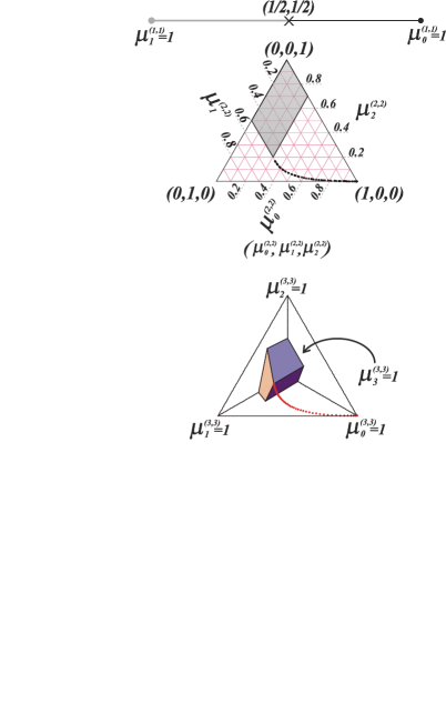
Figure 1: The simplices of symmetric states for the cases of $(\alpha,\beta)$, $\alpha=\beta=1,2,3$, respectively. The equilateral triangle has been marked with contour lines, on each of which one of the parameters is constant. The set of PPT states is indicated by the grey line segment in the top graph, the shaded area of the $(2,2)$ triangle and the filled polygon which obscures the $\mu^{(3,3)}_{3}=1$ vertex in the $(3,3)$ tetrahedral space. In all graphs only the projector of highest spin is within the PPT set. For all three cases, the set of all possible down-conversion states is a curve ending at the boundary of the PPT set, shown by the solid black line for the (1,1) space, and by the dotted curves for the (2,2) and (3,3) spaces. The position of the state on the curve is determined by the parameter $\xi=(1-\eta)\tanh(\kappa t)$.

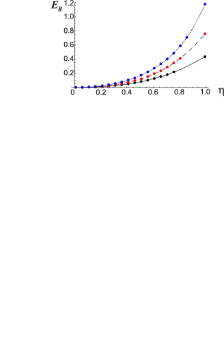
Figure 2: Lower bounds to the relative entropy of entanglement for down-conversion states with initial average photon numbers of $0.5$ (solid), $1$ (dashed), and $3$ (dotted line) subject to loss, evaluating the sum of Eq. (21) up to a truncation of $\alpha,\beta\leq 5$. This gives a good approximation to the total entanglement for average photon numbers before loss up to about $3$.

Fig. 1 also shows the curves traced by the down-conversion states when they are subject to loss. As discussed above, the position of the states on the curve is determined by the single parameter $\xi$. For perfect transmission corresponding to $\eta=1$ the quantum state in an $\alpha=\beta$ photon space has $\mu^{(\alpha,\beta)}_{0}=1$ for all values of $t$, corresponding to maximal entanglement. As losses are increased the state migrates towards the PPT boundary. It is an important immediate consequence of Eq. (18) that for all losses $\eta>0$, the number $\mu^{(\alpha,\alpha)}_{0}$ is always greater than $1/2$ for any finite $t$ and for all $\alpha$. For any finite $t$, $\mu^{(\alpha,\alpha)}_{0}\rightarrow 1/2$ as $\xi\rightarrow 1$ (which corresponds to a limit of zero transmission time and infinite interaction time). This holds true for $(\alpha,\alpha)=(1,1)$, but also for higher values of $\alpha$: the state remains outside the PPT set for any non-vanishing $t$ and for arbitrarily high losses. Therefore, the above results show that there is always some entanglement in the down-conversion state, as quantified in terms of the relative entropy of entanglement. As a corollary, which one can already infer from the lowest dimensional subspace, $(\alpha,\alpha)=(1,1)$, there is actually distillable entanglement in the down-conversion state, regardless of how lossy the transmission from the source to the detector.

We now proceed to quantify the entanglement in the states more explicitly. Since $E_{R}$ is convex and the set of symmetric PPT states is convex, finding the closest state $\sigma$ amounts to solving a convex optimisation problem. For different values of $\alpha,\beta$ the quantities $S(\rho^{(\alpha,\beta)}||\sigma^{(\alpha,\beta)})$ have been evaluated, where $\sigma^{(\alpha,\beta)}$ denotes the PPT state which is the unique global minimum in the convex optimization problem, i.e., the PPT state closest to the down-conversion state. For generic states, this optimization problem would still be convex, yet, the dimensionality of state space grows as $(\alpha+1)^{2}(\beta+1)^{2}-1$. The symmetry dramatically reduces the dimensionality of the constraint set to searched to $\text{min}(\alpha,\beta)$, and thus makes the quantification of the entanglement a feasible task. For instance, for a state with three photons on each side, one has to consider only three objective variables instead of 255. The total relative entropy of entanglement is given by the expression

$$E_{R}(\rho)=\sum_{\alpha,\beta=0}^{\infty}P{(\alpha,\beta)}E_{R}(\rho^{(\alpha,\beta)}).$$ (21)

The average photon number before loss $N$ is related to the interaction time $t$ as $N=2\sinh^{2}(\kappa t)$. The average photon number after loss is $n=\eta N$. Fig. 2 shows the relative entropy of entanglement calculated as described above for $N=0.5$, $N=1$ and $N=3$. One sees that significant entanglement remains even for substantial losses.

IV Conclusions

We have shown how symmetry considerations make possible the quantification of entanglement for states produced by parametric down-conversion and subject to losses. The resilience of the entanglement of these multi-photon states under photon loss makes them an excellent system for the experimental demonstration of entanglement of large photon numbers eisenberg and good candidates for quantum communication schemes durkin .

- (1) For recent reviews see A. Zeilinger, Rev. Mod. Phys. 71, S288 (1999); N. Gisin, G. Ribordy, W. Tittel, and H. Zbinden, Rev. Mod. Phys. 74, 145 (2002); D. Bouwmeester, A. Ekert, and A. Zeilinger, The Physics of Quantum Information (Springer, Heidelberg-Berlin-New York, 2000).
- (2) P.G. Kwiat, K. Mattle, H. Weinfurter, A. Zeilinger, A.V. Sergienko, and Y. Shih, Phys. Rev. Lett. 75, 4337 (1995).
- (3) A. Lamas-Linares, J.C. Howell, and D. Bouwmeester, Nature 412, 887 (2001); F. De Martini, G. Di Giuseppe, and S. Pádua, Phys. Rev. Lett. 87, 150401 (2001)
- (4) H.S. Eisenberg, G. Khoury, G.A. Durkin, C. Simon, and D. Bouwmeester, Phys. Rev. Lett. 93, 193901 (2004).
- (5) G.A. Durkin, C. Simon, and D. Bouwmeester, Phys. Rev. Lett. 88, 187902 (2002).
- (6) C. Simon and D. Bouwmeester, Phys. Rev. Lett. 91, 053601 (2003).
- (7) M.D. Reid, W.J. Munro, and F. De Martini, Phys. Rev. A 66, 033801 (2002); A.B. U’Ren, K. Banaszek, and I.A. Walmsley, Quant. Inf. Comp. 3, 480 (2003).
- (8) J.C. Howell, A. Lamas-Linares, and D. Bouwmeester, Phys. Rev. Lett. 88, 030401 (2002).
- (9) R.F. Werner, Phys. Rev. A 40, 4277 (1989).
- (10) E.M. Rains, Phys. Rev. A 60, 179 (1999).
- (11) J. Eisert, T. Felbinger, P. Papadopoulos, M.B. Plenio, and M. Wilkens, Phys. Rev. Lett. 84, 1611 (2000); B.M. Terhal and K.G.H. Vollbrecht, Phys. Rev. Lett. 85, 2625 (2000).
- (12) K. Audenaert, J. Eisert, E. Jané, M.B. Plenio, S. Virmani, and B. De Moor, Phys. Rev. Lett. 87, 217902 (2001); K. Audenaert, B. De Moor, K.G.H. Vollbrecht, and R.F. Werner, Phys. Rev. A 66, 032310 (2002).
- (13) K.G.H. Vollbrecht and R.F. Werner, Phys. Rev. A 64, 062307 (2001).
- (14) H.F. Jones, Groups, Representations and Physics, 2nd edition (Institute of Physics, London, 1998).
- (15) J. Schliemann, Phys. Rev. A 68, 012309 (2003).
- (16) The measures distillable entanglement and entanglement cost specify certain optimal conversion rates: these are the rates that can be achieved in an asymptotic extraction of and preparation procedure starting from maximally entangled qubit pairs. These procedures are thought to be implemented by employing local quantum operations and classical communication (LOCC) only Bennett ; Rains .
- (17) C.H. Bennett, D.P. DiVincenzo, J.A. Smolin, and W.K. Wootters, Phys. Rev. A 54, 3824 (1996).
- (18) V. Vedral, M.B. Plenio, M.A. Rippin, and P.L. Knight, Phys. Rev. Lett. 78, 2275 (1997); V. Vedral and M.B. Plenio, Phys. Rev. A 57, 1619 (1998); J. Eisert, C. Simon, and M.B. Plenio, J. Phys. A 35, 3911 (2002).
- (19) This is the transposition with respect to one part of a bi-partite quantum system. If the resulting partial transpose is a positive operator, then the original state is said to have a positive partial transpose. See A. Peres, Phys. Rev. Lett. 77, 1413 (1996).
- (20) M. Horodecki, P. Horodecki, and R. Horodecki, Phys. Rev. Lett. 80, 5239 (1998).
- (21) With the methods of Refs. Regul , the asymptotic versions would in principle also be accessible for this class of states.
- (22) The set of bi-partite PPT states with symmetry has been investigated independently by B. Hendriks (Diploma thesis, University of Braunschweig, 2002) under the supervision of R.F. Werner.