Dissipation in systems of linear and nonlinear quantum scissors

Abstract

We analyze truncation of coherent states up to a single-photon Fock state by applying linear quantum scissors, utilizing the projection synthesis in a linear optical system, and nonlinear quantum scissors, implemented by periodically driven cavity with a Kerr medium. Dissipation effects on optical truncation are studied in the Langevin and master equation approaches. Formulas for the fidelity of lossy quantum scissors are found.

Keywords: Quantum state engineering, Kerr effect, qubit generation, finite-dimensional coherent states

I Introduction

The breathtaking advances in quantum computation and quantum information processing in the last decade Nie00 have stimulated progress in quantum optical state generation and engineering JMO97 . Among various schemes, the proposal of Pegg, Phillips and Barnett Peg98 ; Bar99 of the optical state truncation via projection synthesis has attracted considerable interest Bab02 –Mir03 due to the simplicity of the scheme to generate and teleport ‘flying’ qubits defined as a running wave superpositions of zero- and single-photon states. The scheme is referred to as linear quantum scissors (LQS) since the coherent state entering the system is truncated in its Fock expansion to the first two terms using only linear optical elements and performing conditional photon counting. The optical state truncation can also be realized in systems comprising nonlinear elements including a Kerr medium Leo94 ; Dar00 . Such systems will be referred to as nonlinear quantum scissors (NQS). Both LQS Kon00 ; Vil01 and NQS Leo97 ; Mir96 can be generalized for the generation of a superposition of $N$ states. It is worth noting that there are fundamental differences between the states truncated by the LQS and NQS Mir01 .

In this paper we analyze the effects of dissipation on state truncation by quantum scissors. Various kinds of losses in quantum scissors have already been analyzed including: inefficiency and dark counts of photodetectors Bar99 ; Vil99 ; Par00 ; Ozd01 ; Ozd02a , non-ideal single-photon sources Ozd01 ; Ozd02a , mode mismatch Ozd02b , and losses in beam splitters Vil99 . Özdemir et al. Ozd01 ; Ozd02a ; Ozd02b demonstrated that the LQS exhibit surprisingly high fidelity in realistic setups even with conventional photon counters so long as the amplitude of the input coherent state is sufficiently small. LQS has recently been realized experimentally by Babichev et al. Bab02 and Resch et al. Res02 , although only in the low-intensity regime. The effect of losses on the optical truncation in NQS has been studied for zero-temperature reservoir Leo01 and imperfect photodetection Dar00 .

These studies of losses in LQS (with few exceptions, e.g., for Vil99 ) have been based on the quantum detection and estimation theory using the positive operator valued measures (POVM) Hel76 . In quantum-optics textbooks (see, e.g., Lou73 ; Per91 ), the quantum-statistical properties of dissipative systems are usually treated in three ways, by applying (i) the Langevin (Langevin-Heisenberg) equations of motion with stochastic forces, (ii) the master equation for the density matrix, and (iii) the classical Fokker-Planck equation for quasiprobability distribution. In the next section we will apply the Langevin approach to describe dissipative LQS, while in section 3 we shall use the master equation approach to study dissipative NQS.

II Lossy linear quantum scissors in the Langevin approach

The linear quantum scissors device of Pegg, Phillips and Barnett Peg98 ; Bar99 is a simple physical system for optical state truncation based only on linear optical elements (two beam splitters BS1 and BS2) and two photodetectors (D2 and D3) as depicted in figure 1. If the input modes $a_{1}$ and $a_{2}$ are in the single-photon and vacuum states, respectively, and one photon is detected at D2 but no photons at D3, then the lossless LQS device with 50/50 beam splitters truncates the input coherent state $|\alpha\rangle$ in mode $b_{3}$ to the following superposition of vacuum and single-photon states in mode $b_{1}$

$$|\alpha_{{\rm trunc}}{\rangle}_{b1}=N^{\prime}\ _{c2c3}\langle 10|\psi_{{\rm out}}{\rangle}_{b1c2c3}=\frac{|0\rangle_{b1}+\alpha|1\rangle_{b1}}{\sqrt{1+|\alpha|^{2}}}$$ (1)

where $\alpha$ is the complex amplitude and $N^{\prime}$ is a renormalization constant. The state (1) is referred to as the truncated two-dimensional (or two-level) coherent state since it is the normalized superposition of the first two terms of Fock expansion of the Glauber coherent state. By introducing a new variable $\bar{\alpha}$ such that $\cos(|\bar{\alpha}|)=1/\sqrt{1+|\alpha|^{2}}$ and $\sin(|\bar{\alpha}|)=|\alpha|/\sqrt{1+|\alpha|^{2}}$, and $\varphi={\rm Arg}\alpha$, state (1) can be rewritten as

$$|{\alpha}_{\rm trunc}\rangle=\cos(|\bar{\alpha}|)|0\rangle+e^{i\varphi}\sin(|\bar{\alpha}|)|1\rangle$$ (2)

where, for brevity, subscript $b_{1}$ is skipped. If the $j$th ($j=1,2$) beam splitter has an arbitrary but real transmission coefficient $t_{j}$ and an imaginary reflection coefficient $r_{j}$, then the LQS generates the state Ozd01

$$|\psi{\rangle}_{b1}=\frac{|r_{1}t_{2}||0\rangle_{b1}+\alpha|r_{2}t_{1}||1\rangle_{b1}}{\sqrt{|r_{1}t_{2}|^{2}+|\alpha|^{2}|r_{2}t_{1}|^{2}}}.$$ (3)

This state evolves into the truncated coherent state (1) by assuming identical BSs ($r_{1}=r_{2}$ and $t_{1}=t_{2}$).

In general, the transmission and reflection coefficients of a perfect BSs obey the conditions $\left|t\right|^{2}+\left|r\right|^{2}=1$ and $tr^{\ast}+t^{\ast}r=0$, implied by the unitarity of BS transformation. By including dissipation, these conditions can be violated. Thus, the main goal of this section is to analyze the deterioration of the truncation process due to the noise introduced by lossy beam splitters and also by inefficient photodetectors. In the simplest approach, one can model the BS losses and finite detector efficiency by adding to our system additional beam splitters, then all components of the system (including the new BSs) can be assumed perfect. Here, we apply another standard approach of the quantum theory of damping based on the Langevin noise operators Lou73 ; Per91 . We follow the analyses of Barnett et al. Bar96 ; Bar98 and Villas-Bôas et al. Vil99 . The lossy BS1 transforms the input annihilation operators $\hat{a}_{j}$ into the output $\hat{b}_{j}$ as follows Bar96 ; Bar98

$$\hat{a}_{1} = t_{1}^{\ast}\hat{b}_{1}+r_{1}^{\ast}\hat{b}_{2}+\hat{L}_{a1},$$

$$\hat{a}_{2} = r_{1}^{\ast}\hat{b}_{1}+t_{1}^{\ast}\hat{b}_{2}+\hat{L}_{a2}$$ (4)

where we use the notation of figure 1, and $\hat{L}_{a1}$ and $\hat{L}_{a2}$ are the Langevin noise (force) operators satisfying the following commutation relations

$$[\hat{L}_{a1},\hat{L}_{a1}^{{\dagger}}] = [\hat{L}_{a2},\hat{L}_{a2}^{{\dagger}}]=1-|t_{1}|^{2}-|r_{1}|^{2}\equiv\Gamma_{1},$$

$$[\hat{L}_{a1},\hat{L}_{a2}^{{\dagger}}] = [\hat{L}_{a2},\hat{L}_{a1}^{{\dagger}}]=-(t_{1}r_{1}^{\ast}+t_{1}^{\ast}r_{1})\equiv-\Omega_{1}.$$ (5)

The transformation between the input ($\hat{b}_{j}$) and output ($\hat{c}_{j}$) annihilation operators of the lossy BS2 together with effect of finite efficiency ($\eta\equiv\eta_{1}=\eta_{2}$) of detectors generalizes to Vil99

$$\hat{b}_{2} = \sqrt{\eta}t_{2}^{\ast}\hat{c}_{2}+\sqrt{\eta}r_{2}^{\ast}\hat{c}_{3}+\hat{L}_{b2},$$

$$\hat{b}_{3} = \sqrt{\eta}r_{2}^{\ast}\hat{c}_{2}+\sqrt{\eta}t_{2}^{\ast}\hat{c}_{3}+\hat{L}_{b3}$$ (6)

where the Langevin noise operators $\hat{L}_{b2}$ and $\hat{L}_{b3}$ obey

$$[\hat{L}_{b2},\hat{L}_{b2}^{{\dagger}}] = [\hat{L}_{b3},\hat{L}_{b3}^{{\dagger}}]=\eta\Gamma_{2}+(1-\eta)\equiv x,$$

$$[\hat{L}_{b2},\hat{L}_{b3}^{{\dagger}}] = [\hat{L}_{b3},\hat{L}_{b2}^{{\dagger}}]=-\eta\Omega_{2}.$$ (7)

In (5) and (7), $\Omega_{j}=t_{j}r_{j}^{\ast}+t_{j}^{\ast}r_{j}$ and $\Gamma_{j}=1-|t_{j}|^{2}-|r_{j}|^{2}$ are the $j$th beam splitter phase and amplitude dissipation coefficients, respectively, which vanish for perfect beam splitters. For simplicity, we assume that the BSs are identical ($r_{1}=r_{2}\equiv r,$ $t_{1}=t_{2}\equiv t$) and they cause only amplitude damping ($\Gamma\equiv\Gamma_{1}=\Gamma_{2}\neq 0)$ without introducing phase noise ($\Omega_{1}=\Omega_{2}=0$). By applying the transformations (4) and (6) for the input state $|\psi_{{\rm in}}{\rangle}_{a1a2b3}=|1\rangle_{a1}|0{\rangle}_{a2}|\alpha{\rangle}_{b3}$ and performing the conditional measurement (projection synthesis) on modes $c_{2}$ and $c_{3}$ (as shown in figure 1), one finds that the state of the output mode $b_{1}$ of the LQS is entangled with the environment as follows Vil99

$$|\psi{\rangle}_{b1E} = N^{\prime\prime}\ _{c2c3}\langle 10|\psi_{{\rm out}}{\rangle}_{b1c2c3E}$$ (8)

$$= N(|0{\rangle}_{b1}|\mathbf{\Lambda}_{0}\rangle_{E}+\alpha|1{\rangle}_{b1}|\mathbf{\Lambda}_{1}\rangle_{E})$$

where we write compactly the environmental states as

$$|\mathbf{\Lambda}_{0}\rangle_{E} = \sqrt{\eta}r(t+\alpha r\hat{L}_{a2}^{{\dagger}}+\alpha\hat{L}_{a1}^{{\dagger}})\exp(\alpha\hat{L}_{b3}^{{\dagger}})|\mathbf{0}{\rangle}_{E},$$

$$|\mathbf{\Lambda}_{1}\rangle_{E} = \sqrt{\eta}rt\exp(\alpha\hat{L}_{b3}^{{\dagger}})|\mathbf{0}{\rangle}_{E}$$ (9)

and the normalization $N$ is given by

$$N=\{\eta|r|^{2}\ |\alpha|^{2}e^{x|\alpha|^{2}}[|t|^{2}(|\alpha|^{-2}+1)+|r|^{2}x+\Gamma]\}^{-1/2}$$ (10)

and $N^{\prime\prime}$ is a renormalization constant. The fidelity of the output state (8) of the lossy LQS to a desired perfectly truncated state, given by (1), can be calculated from

$$F\equiv||_{b1}\langle\alpha_{{\rm trunc}}|\psi{\rangle}_{b1E}||^{2}$$ (11)

which leads us to the following relation

$$F = N^{2}\eta|r|^{2}\ \exp(x|\alpha|^{2})$$ (12)

$$\times\left(|t|^{2}(|\alpha|^{2}+1)+\frac{|\alpha|^{2}}{1+|\alpha|^{2}}(|r|^{2}x+\Gamma)\right)$$

where the normalization $N$ is given by (10). By defining $R=1/|\alpha|^{2}$, equation (12) can be simplified to

$$F=1-\frac{(\eta\Gamma+1-\eta)|r|^{2}+\Gamma}{(1+R)[(\eta\Gamma+1-\eta)|r|^{2}+\Gamma+|t|^{2}(1+R)]}$$ (13)

where $x=\eta\Gamma+(1-\eta)$. In a special case for 50/50 BSs, $|r|^{2}=|t|^{2}$, our solution simplifies to that of Villas-Bôas et al. (private , note that the corresponding fidelity in Vil99 is misprinted). By neglecting losses caused by beam splitters, solution (13) is further reduced to the well-known Pegg-Phillips-Barnett fidelity Peg98

$$F=1-\frac{|\alpha|^{4}(1-\eta)}{(1+|\alpha|^{2})[1+|\alpha|^{2}(2-\eta)]}.$$ (14)

By assuming also perfect detectors, the fidelity becomes unity, as expected.

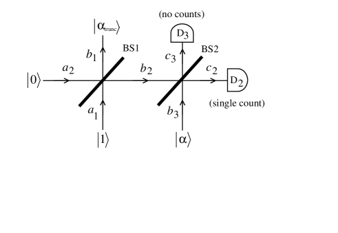
Figure 1: Scheme of linear quantum scissors: $|\alpha\rangle$ is the input coherent state, $|\alpha_{\rm trunc}\rangle$ is the output truncated coherent state, $|0\rangle$ and $|1\rangle$ are vacuum and single-photon states, respectively; BS1 and BS2 are beam splitters; D2 and D3 are photon detectors. For successful truncation process, one of the detectors should detect one photon, while the other – no photons.

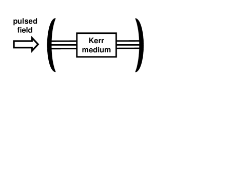
Figure 2: Scheme of nonlinear quantum scissors: cavity with a Kerr medium is pumped by external ultra-short pulses of laser light.

III Lossy nonlinear quantum scissors in the master equation approach

In nonlinear quantum scissors scheme, schematically depicted in figure 2, a cavity mode is pumped by an external classical pulsed laser field, described by Hamiltonian $\hat{H}_{K}$, and is interacting with a Kerr medium, described by Hamiltonian $\hat{H}_{NL}$. Thus, the whole system Hamiltonian is given by Leo94 ; Leo01

$$\hat{H}_{S}=\hat{H}_{0}+\hat{H}_{NL}+\hat{H}_{K}$$ (15)

where

$$\hat{H}_{NL} = \hbar\frac{\kappa}{2}(\hat{a}^{{\dagger}})^{2}\hat{a}^{2},$$ (16)

$$\hat{H}_{K} = \hbar\epsilon(\hat{a}^{{\dagger}}+\hat{a})\sum_{k=-\infty}^{\infty}\delta(t-kT_{K})$$ (17)

and the free Hamiltonian of the system is $\hat{H}_{0}=\hbar\omega\hat{a}^{{\dagger}}\hat{a}$. In Eq. (16), $\hat{a}$ is the annihilation operator for a cavity mode at frequency $\omega$, and $\kappa$ is the nonlinear coupling proportional to the third-order susceptibility of the Kerr medium. In (17), Dirac $\delta$ functions describe external ultra-short light pulses (kicks); real parameter $\epsilon$ is the strength of the interaction of the cavity mode with the external field; $T_{K}$ is the period of free evolution between the kicks. The truncation process in the system, given by (15), occurs if (i) $T_{K}\gg T_{\mathrm{round-trip}}\gg 2\pi/\omega$, where $\omega$ is the light frequency and $T_{\mathrm{round-trip}}$ is the round-trip time of the light in the cavity, and (ii) the kicks are much weaker than the Kerr nonlinear interaction, $\epsilon\ll\kappa$. As shown in Refs. Leo94 ; Leo97 , the state generated by the NQS is a two-dimensional coherent state Buz92 ; Mir94 of the form

$$|\bar{\alpha}_{\rm trunc}\rangle\approx\cos(|\bar{\alpha}|)|0\rangle-i\sin(|\bar{\alpha}|)|1\rangle$$ (18)

where $\bar{\alpha}=-ik\epsilon$. Dissipation of the NQS system is modelled by its coupling to a reservoir of oscillators (heat bath) described by the Hamiltonian

$$\hat{H} = \hat{H}_{S}+\hat{H}_{R}+\hat{H}_{SR},$$ (19)

$$\hat{H}_{SR} = \hbar\sum_{j}(g_{j}\hat{a}\hat{b}_{j}^{{\dagger}}+g_{j}^{\ast}\hat{a}^{{\dagger}}\hat{b}_{j})$$ (20)

where $\hat{H}_{S}$ is given by (15) and $\hat{H}_{R}=\hbar\sum_{j}\chi_{j}\hat{b}_{j}^{{\dagger}}\hat{b}_{j}$ is the free Hamiltonian of the reservoir, where $\hat{b}_{j}$ is the boson annihilation operator of the $j$th reservoir oscillator. By applying the standard methods of the quantum theory of damping Lou73 , one finds that the NQS evolution between the kicks is governed under the Markov approximation by the following master equation in the interaction picture

$$\frac{\partial}{\partial t}\hat{\rho}=-i\frac{\kappa}{2}[(\hat{a}^{{\dagger}})^{2}\hat{a}^{2},\hat{\rho}]-\frac{\gamma}{2}([\hat{a}^{{\dagger}},\hat{a}\hat{\rho}]+{\rm h.c.})+\gamma\bar{n}[\hat{a}^{{\dagger}},[\hat{\rho},\hat{a}]]$$ (21)

where $\gamma$ is the damping constant and $\bar{n}$ is the mean number of thermal photons, $\bar{n}=\{\exp[\hbar\omega/(k_{B}T)]-1\}^{-1}$, at the reservoir temperature $T$, where $k_{B}$ is the Boltzmann constant. Let the kick be applied at time $t_{K}$, then the solution of Eq. (21) for any time $t$ after $t_{K}$ but before moment $t_{K}+T_{K}$ is the same as the solution for the ordinary damped anharmonic oscillator Dan89 ; Per90 ; Gan91 with the initial state given at time $t_{K}$. We can write the solution compactly as $(\rho_{nm}\equiv\langle n|\hat{\rho}|m\rangle)$:

$$\rho_{nm}(t_{K}+t) = \exp[\frac{\gamma t}{2}+i(n-m)\kappa t]E_{n-m}^{n+m+1}(t)$$

$$\times\sum_{l=0}^{\infty}\rho_{n+l,m+l}(t_{K})\sqrt{C_{n}^{n+l}C_{m}^{m+l}}\bar{g}_{n-m}^{l}(t)$$

$$\times F[-n,-m,l+1;\frac{4\bar{n}(\bar{n}+1)}{\Delta_{n-m}^{2}}\sinh^{2}t_{n-m}]$$

where $F$ is the hypergeometric function, $C_{y}^{x}$ are binomial coefficients, $t_{x}=\gamma\Delta_{x}t/2$ and

$$\bar{g}_{x}(t) = \frac{2(\bar{n}+1)}{\Omega_{x}+\Delta_{x}\coth t_{x}},$$

$$E_{x}(t) = \frac{\Delta_{x}}{\Omega_{x}\sinh t_{x}+\Delta_{x}\cosh t_{x}}$$ (23)

with $\Delta_{x}=\sqrt{\Omega_{x}^{2}-4\bar{n}(\bar{n}+1)}$ and $\Omega_{x}=1+2\bar{n}+i\kappa x/\gamma.$ By assuming the reservoir to be at zero temperature, the solution (III) reduces to Mil86 ; Per88 ; Mil91

$$\rho_{nm}(\tau_{K}+\tau)=\exp[i(n-m)\frac{\tau}{2}]f_{n-m}^{(n+m)/2}(\tau)$$ (24)

$$\quad\times\sum_{l=0}^{\infty}\rho_{n+l,m+l}(\tau_{K})\sqrt{C_{n}^{n+l}C_{m}^{m+l}}\left(\frac{\lambda[1-f_{n-m}(\tau)]}{\lambda+i(n-m)}\right)^{l}$$

where $\tau$ is the scaled time given by $\tau=\kappa t$, so $\tau_{K}=\kappa t_{K}$. Moreover, $\lambda=\gamma/\kappa$, and $f_{x}(\tau)=\exp[-(\lambda+ix)\tau]$. For a lossless anharmonic oscillator, i.e. for $\lambda=0$, the solution (24) further simplifies to

$$\rho_{nm}(\tau_{K}+\tau)=\exp\{i[n(n-1)-m(m-1)]\frac{\tau}{2}\}\rho_{nm}(\tau_{K})$$ (25)

Solution (III) describes the evolution of the NQS between the kicks only. On the other hand, the evolution at each kick is given by

$$\lim_{\delta\rightarrow 0}\langle n|\hat{\rho}(t_{K}+\delta)|m\rangle$$ (26)

$$\quad\quad=\lim_{\delta\rightarrow 0}\sum_{n^{\prime},m^{\prime}=0}^{\infty}\!\!U_{nn^{\prime}}\langle n^{\prime}|\hat{\rho}(t_{K}-\delta)|m^{\prime}\rangle U_{mm^{\prime}}^{\ast}$$

where

$$U_{nm}=\langle n|\hat{U}|m\rangle=\langle n|\exp[-i\epsilon(\hat{a}^{{\dagger}}+\hat{a})]|m\rangle$$ (27)

in analogy to the Milburn-Holmes transformation for the pulsed parametric amplifier with a Kerr nonlinearity Mil91 . By observing that $\hat{U}$ is the displacement operator $\hat{U}=\exp[-i\epsilon(\hat{a}^{{\dagger}}+\hat{a})]=\hat{D}(-i\epsilon)$, we can use the well-known Cahill-Glauber Cah69 formulas leading for $n\geq m$ to

$$U_{nm}=e^{-\epsilon^{2}/2}\sqrt{\frac{m!}{n!}}(-i\epsilon)^{n-m}L_{m}^{n-m}(\epsilon^{2})$$ (28)

and for $n<m$ to

$$U_{nm}=e^{-\epsilon^{2}/2}\sqrt{\frac{n!}{m!}}(i\epsilon)^{m-n}L_{n}^{m-n}(\epsilon^{2})$$ (29)

where $L_{x}^{y}(z)$ is an associated Laguerre polynomial. Thus, we have a complete solution to describe the effects of dissipation on, in particular, the truncation fidelity after the $k$th kick, which is given by

$$\bar{F}(t) = \langle\bar{\alpha}_{\rm trunc}|\hat{\rho}(t)|\bar{\alpha}_{\rm trunc}\rangle$$

$$= \cos^{2}(k\epsilon)\rho_{00}(t)+\sin(2k\epsilon)\mathrm{Im}\rho_{01}(t)+\sin^{2}(k\epsilon)\rho_{11}(t)$$

where the perfectly truncated state $|\bar{\alpha}\rangle_{\mathrm{NQS}}$ was applied according to (18).

IV CONCLUSIONS

We studied dissipative quantum scissors systems for truncation of a Glauber (infinite-dimensional) coherent state to a superposition of vacuum and single-photon Fock states (two-dimensional coherent state). We have contrasted the Pegg-Phillips-Barnett quantum scissors based on linear optical elements and the Leoński-Tanaś quantum scissors comprising nonlinear Kerr medium. We analyzed the effects of dissipation on truncation fidelity in the linear scissors within the Langevin noise operator approach and in the nonlinear system in the master equation approach.

Acknowledgements. AM warmly thanks Şahin K. Özdemir, Masato Koashi, and Nobuyuki Imoto for long and stimulating collaboration on experimental realization of quantum scissors. The authors also thank Ryszard Tanaś for helpful discussions.

References

• (1) M A Nielsen and I L Chuang 2000 Quantum Computation and Quantum Information (Cambridge: University Press)
• (2) Special issue on Quantum State Preparation and Measurement, 1997 J. Mod. Opt. 44 No. 11/12
• (3) Pegg D T, Phillips L S and Barnett S M 1998 Phys. Rev. Lett. 81 1604
• (4) Barnett S M and Pegg D T 1999 Phys. Rev. A 60 4965
• (5) Babichev S A, Ries J, and Lvovsky A I 2003 Europhys. Lett. 64 1
• (6) Resch K J, Lundeen J S, and Steinberg A M 2002 Phys. Rev. Lett. 88 113601
• (7) Villas-Bôas C J, de Almeida N G, and Moussa M H Y 1999 Phys. Rev. A 60 2759
• (8) Paris M G A 2000 Phys. Rev. A 62 033813
• (9) Özdemir Ş K, Miranowicz A, Koashi M, and Imoto N 2001 Phys. Rev. A 64 063818
• (10) Özdemir Ş K, Miranowicz A, Koashi M, and Imoto N 2002 J. Mod. Opt. 49 977
• (11) Özdemir Ş K, Miranowicz A, Koashi M, and Imoto N 2002 Phys Rev A 66 053809
• (12) Koniorczyk M, Kurucz Z, Gabris A, and Janszky J 2000 Phys Rev A 62 013802
• (13) Villas-Bôas C J, Guimarǎes Y, Moussa M H Y, and Baseia B 2001 Phys. Rev. A 63 055801
• (14) Leoński W and Tanaś R 1994 Phys. Rev. A 49 R20
• (15) D’Ariano G M, Maccone L, Paris M G A, and Sacchi M F 2000 Phys. Rev. A 61 053817
• (16) Leoński W 1997 Phys. Rev. A 55 3874
• (17) Miranowicz A, Leoński W, Dyrting S, and Tanaś R 1996 Acta Phys. Slov. 46 451
• (18) Miranowicz A, Leoński W, and Imoto N 2001 Adv. Chem. Phys. (New York: Wiley) 119(I) 155
• (19) Leoński W and Miranowicz A 2001 Adv. Chem. Phys. (New York: Wiley) 119(I) 195
• (20) Miranowicz A, Özdemir Ş K, Leoński W, Koashi M, and Imoto N 2003 Proc. of SPIE 5259 47
• (21) Helstrom C W 1976 Quantum Detection and Estimation Theory, (New York: Academic Press)
• (22) Louisell W H 1973 Quantum Statistical Properties of Radiation (New York: Wiley)
• (23) Peřina J 1991 Quantum Statistics of Linear and Nonlinear Optical Phenomena (London: Kluwer)
• (24) Barnett S M, Gilson C R, Huttner B, and Imoto N 1996 Phys. Rev. Lett. 77 1739
• (25) Barnett S, Jeffers J, Gatti A, and Loudon R 1998 Phys. Rev. A 57 2134
• (26) Villas-Bôas C J, de Almeida N G, and Moussa M H Y, private communication.
• (27) Bužek V, Wilson-Gordon A D, Knight P L, and Lai W K 1992 Phys. Rev. A 45 8079
• (28) Miranowicz A, Pia̧tek K, and Tanaś R 1994 Phys. Rev. A 50 3423
• (29) Daniel D J and Milburn G J 1989 Phys. Rev. A 39 4628
• (30) Peřinová V and Lukš A 1988 J. Mod. Opt. 35 1513
• (31) Peřinová V and Lukš A 1990 Phys. Rev. A 41 414
• (32) Gantsog Ts and Tanaś R 1991 Phys. Rev. A 44 2086
• (33) Milburn G J and Holmes C A 1986 Phys. Rev. Lett. 56 2237
• (34) Milburn G J and Holmes C A 1991 Phys. Rev. A 44 4704
• (35) Cahill K E and Glauber R J 1969 Phys. Rev. 177 1857