Violation of Bell inequality and entanglement of decaying Werner states

Abstract

Bell-inequality violation and entanglement, measured by Wootters’ concurrence and negativity, of two qubits initially in Werner or Werner-like states coupled to thermal reservoirs are analyzed within the master equation approach. It is shown how this simple decoherence process leads to generation of states manifesting the relativity of two-qubit entanglement measures.

I Introduction

Quantum nonlocality, responsible for violation of Bell-type inequalities bell ; clauser , and entanglement (inseparability) are the fundamental resources of modern quantum-information theory and still the most surprising features of quantum mechanics (see, e.g., tittel ). It is therefore desirable to investigate the degrees of the Bell-inequality violation and of the entanglement of a quantum state not only in relation to efficiency of quantum-information processing, but also to understand better subtle aspects of the physical nature.

It is well-known that pure states gisin or a mixture of two Bell states violate Bell inequalities whenever they are entangled. So, one could naively think that the only mixed states that do not violate the Bell inequalities are separable states. However, Werner werner demonstrated the existence of entangled states which do not violate any Bell-type inequality. The standard two-qubit Werner state is defined by werner

$${\rho}_{Y}^{(p)}(0) = p|Y\rangle\langle Y|+\frac{1-p}{4}I\otimes{I}$$ (1)

being a mixture for $p\in\langle 0,1\rangle$ of the singlet state $|Y\rangle=(|01\rangle-|10\rangle)/\sqrt{2}$ and the separable maximally mixed state, given by $I\otimes I$, where $I$ is the identity operator of a single qubit. Definition (1) is often generalized to include mixtures of any maximally entangled state (MES) instead of the singlet state only. So, e.g., one can analyze the Werner-like state defined by munro ; ghosh ; wei1

$${\rho}_{X}^{(p)}(0) = p|X\rangle\langle X|+\frac{1-p}{4}I\otimes I,$$ (2)

as a convex combination of the Bell state $|X\rangle=(|00\rangle+|11\rangle)/\sqrt{2}$ and $I\otimes I$. The original Werner state (1), contrary to (2), is invariant if both qubits are subjected to same unitary transformation, say $U\otimes U$. Nevertheless, for a given $p$, both states (1) and (2) exhibit the same entanglement properties, thus (2) is also referred to as the Werner state munro ; ghosh ; wei1 . In addition to the fact that the Werner states can be entangled without violating any Bell inequality for some values of parameter $p$, they can still be used for quantum-information processing including teleportation popescu ; lee . Moreover, the Werner states, given by (1) and (2), can be considered maximally entangled mixed states of two qubits ishizaka ; munro in the sense that their degree of entanglement cannot be increased by any unitary operations, and they have the maximum degree of entanglement for a given linear entropy (and vice versa).

We will study the effects of a lossy environment, modelled by thermal reservoirs, on the Bell-inequality violation and on the entanglement of the initial Werner and Werner-like states in the quest for new states including those having different orderings induced by two entanglement measures: concurrence $C$ and negativity $N$ (defined in Sect. IV). The relativity of the entanglement measures was first observed by Eisert and Plenio eisert . They showed numerically, using Monte Carlo simulation, that the condition

$$C(\rho_{1})<C(\rho_{2})\Leftrightarrow N(\rho_{1})<N(\rho_{2})$$ (3)

can be violated by some two-qubit mixed states, although it is satisfied if $\rho_{1}$ and $\rho_{2}$ are the Werner states or pure states. Virmani and Plenio virmani demonstrated that all good asymptotic entanglement measures are either identical or impose different orderings of quantum states. The problem of relativity of the entanglement measures was also studied in Refs. zyczkowski99 ; verstraete ; zyczkowski02 ; wei1 ; wei2 . Here, in particular, we present analytical examples of different orderings imposed by the concurrence and negativity for two-qubit states, which violate the Bell inequality to the same degree.

The Letter is organized as follows. In Sect. II, we discuss a dissipative model and give a general solution for two decaying qubits initially in the Werner states. A comparative study of the Bell-inequality violation and entanglement of various decaying states are given is Sects. III and IV, respectively. A final comparison and conclusions are given in Sect. V.

II Model for loss mechanism

We analyze evolution of two initially correlated qubits subjected to dissipation modelled by their coupling to thermal reservoirs (phonon baths) as described by the following Hamiltonian

$${H}=H_{S}+\hbar\sum_{k,n}\Omega_{n}^{(k)}({b}_{n}^{(k)})^{{\dagger}}{b}_{n}^{(k)}+\hbar\sum_{k,n}[g_{n}^{(k)}{a}_{k}^{{\dagger}}{b}_{n}^{(k)}+\mathrm{h.c.}]$$ (4)

which is the sum of Hamiltonians for the system, $H_{S}$, reservoirs and the coupling between them, respectively. It is a prototype model, where qubits can be implemented in various ways, e.g., by single-cavity modes restricted in the Hilbert space spanned by the two lowest Fock states (see, e.g., giovannetti ). In (4), ${a}_{k}$ is the annihilation operator for the $k$th ($k=1,2$) qubit at the frequency $\omega_{k}$; ${b}_{n}^{(k)}$ is the annihilation operator for the $n$th oscillator in the $k$th reservoir at the frequency $\Omega_{n}^{(k)}$, and $g_{n}^{(k)}$ are the coupling constants of the reservoir oscillators. We assume no direct interaction between the qubits, thus the system Hamiltonian is simply given by $H_{S}=\hbar\sum_{k=1}^{2}\omega_{k}{a}_{k}^{{\dagger}}{a}_{k}$. The standard master equation for the model reads as

$$\frac{\partial}{\partial t}{\rho} = \frac{1}{i\hbar}[{H}_{S},{\rho}]+\sum_{k=1}^{2}\frac{\gamma_{k}}{2}\{\bar{n}_{k}(2{a}_{k}^{{\dagger}}{\rho}{a}_{k}-{a}_{k}{a}_{k}^{{\dagger}}{\rho}-{\rho}{a}_{k}{a}_{k}^{{\dagger}})$$ (5)

$$+(\bar{n}_{k}+1)(2{a}_{k}{\rho}{a}_{k}^{{\dagger}}-{a}_{k}^{{\dagger}}{a}_{k}{\rho}-{\rho}{a}_{k}^{{\dagger}}{a}_{k})\}$$

where ${\rho}$ is the reduced density operator for the qubits, $\gamma_{k}$ is the damping constant and $\bar{n}_{k}$ is the mean number of thermal photons of the $k$th reservoir. The exact solution of (5) for arbitrary initial conditions and arbitrary-dimensional systems is well known. By confining our analysis to the initial qubit states coupled to the quiet reservoirs ($\bar{n}_{1}=\bar{n}_{2}=0$), the solution in the computational basis $\{|00\rangle,|01\rangle,|10\rangle,|11\rangle\}$ in the interaction picture can compactly be given as

$$\rho(t)=\left[\begin{array}[]{cccc}{h}&f_{1}^{\ast}&f_{2}^{\ast}&\sqrt{g_{1}g_{2}}\rho_{03}\\ f_{1}&h_{1}&\sqrt{g_{1}g_{2}}\rho_{12}&\sqrt{g_{1}}g_{2}\rho_{13}\\ f_{2}&\sqrt{g_{1}g_{2}}\rho_{21}&h_{2}&g_{1}\sqrt{g_{2}}\rho_{23}\\ \sqrt{g_{1}g_{2}}\rho_{30}&\sqrt{g_{1}}g_{2}\rho_{31}&g_{1}\sqrt{g_{2}}\rho_{32}&g_{1}g_{2}\rho_{33}\end{array}\right]$$ (6)

where the elements of the initial density matrix $\rho(0)$ are denoted by $\rho_{2i+k,2j+l}\equiv\langle i,k|\rho(0)|j,l\rangle$; $g_{k}=\exp(-\gamma_{k}t)$ and

$$f_{k} = \sqrt{g_{3-k}}[(1-g_{k})\rho_{3,3-k}+\rho_{k0}],$$

$$h_{k} = g_{3-k}[(1-g_{k})\rho_{33}+\rho_{kk})],$$

$${h} = 1-(h_{1}+h_{2}+g_{1}g_{2}\rho_{33}).$$ (7)

We will apply solution (6) to analyze the effect of dissipation on the Bell-inequality violation and entanglement of the initial Werner states.

III Bell-inequality violation

We will study violation of the Bell inequality due to Clauser, Horne, Shimony and Holt (CHSH) clauser . In a special case of two qubits in an arbitrary mixed state $\rho$, one can apply an effective criterion for violating the Bell inequality:

$$|\mathrm{Tr}\,(\rho\,{\mathcal{B}}_{\mathrm{CHSH}})|\leq 2$$ (8)

where ${\mathcal{B}}_{\mathrm{CHSH}}$ is the Bell operator given by

$${\mathcal{B}}_{\mathrm{CHSH}}=\mathbf{a}\cdot{\boldsymbol{\sigma}}\otimes(\mathbf{b}+\mathbf{b}^{\prime})\cdot{\boldsymbol{\sigma}}+\mathbf{a}^{\prime}\cdot{\boldsymbol{\sigma}}\otimes(\mathbf{b}-\mathbf{b}^{\prime})\cdot{\boldsymbol{\sigma}}$$ (9)

with its mean value maximized over unit vectors $\mathbf{a},\,\mathbf{a}^{\prime},\,\mathbf{b},\,\mathbf{b}^{\prime}$ in $\Re^{3}$. Moreover, ${\boldsymbol{\sigma}}$ is the vector of the Pauli spin matrices $\sigma_{1},\sigma_{2},\sigma_{3}$, and scalar product $\mathbf{a}\cdot{\boldsymbol{\sigma}}$ stands for $\sum\limits_{j=1}^{3}a_{j}\sigma_{j}$. By noting that any $\rho$ can be represented in the Hilbert-Schmidt basis as

$$\rho=\tfrac{1}{4}\left(I\!\otimes I+\mathbf{r}\cdot{\boldsymbol{\sigma}}\otimes I+I\otimes\mathbf{s}\cdot{\boldsymbol{\sigma}}+\!\!\!\sum\limits_{n,m=1}^{3}t_{nm}\,\sigma_{n}\otimes\sigma_{m}\right)$$ (10)

where $\mathbf{r},\mathbf{s}$ are vectors in $\Re^{3}$, Horodecki et al. horodecki1 ; horodecki2 proved that the maximum possible average value of the Bell operator in the state $\rho$ is given by

$$\max_{{\mathcal{B}}_{\mathrm{CHSH}}}\,\mathrm{Tr}\,(\rho\,{\mathcal{B}}_{\mathrm{CHSH}})=2\,\sqrt{M(\rho)}$$ (11)

in terms of $M(\rho)=\max_{j<k}\;\{u_{j}+u_{k}\}$, where $u_{j}$ $(\,j=1,2,3)$ are the eigenvalues of the real symmetric matrix $U_{\rho}=T_{\rho}^{T}\,T_{\rho}$; $T_{\rho}$ is the real matrix formed by the coefficients $t_{nm}=\mathrm{Tr}\,(\rho\,\sigma_{n}\otimes\sigma_{m})$, and $T_{\rho}^{T}$ is the transposition of $T_{\rho}$. Thus, the necessary and sufficient condition for violation of inequality (8) by the density matrix (10) and Bell operator (9) for some choice of $\mathbf{a},\mathbf{a}^{\prime},\mathbf{b},\mathbf{b}^{\prime}$ reads as $M(\rho)>1$ horodecki1 ; horodecki2 . To quantify the degree of the Bell-inequality violation one can use $M(\rho)$, $2\,\sqrt{M(\rho)}$ (see, e.g., ghosh ; jakob ), or $\max\,\{0,\,M(\rho)-1\,\}$ (see, e.g., jakobczyk ). But we propose to use the following quantity

$$B(\rho)\equiv\sqrt{\max\,\{0,\,M(\rho)-1\,\}}$$ (12)

which has a useful property that for any two-qubit pure state it is equal to the entanglement measures such as concurrence and negativity, defined in the next section. As $M(\rho)\leq 2$, it holds $B(\rho)\in\langle 0,1\rangle$, where $B(\rho)=1$ corresponds to the maximal violation of inequality (8) and $B(\rho)=0$ for states admitting the local hidden variable model. The larger value of $B(\rho)>0$ the greater violation of the Bell inequality. Thus, $B(\rho)$ can be used to quantify the degree of the Bell-inequality violation (BIV), and for short it will be referred to as the BIV degree.

The BIV degrees for the initial Werner states ${\rho}_{X}^{(p)}(0)$ and ${\rho}_{Y}^{(p)}(0)$ are the same and equal to

$$B_{X}^{(p)}(0)=B_{Y}^{(p)}(0)=\max\{0,2p^{2}-1\}^{1/2}$$ (13)

implying that the states violate the Bell inequality iff $1/\sqrt{2}<p\leq 1$. By changing the parameter $p$ into $\phi=(1-3p)/2$, (13) goes into another well-known form (see, e.g., horodecki1 ; horodecki2 ). The BIV degree of the maximally entangled states ($p=1$) is also maximal and equal to one as shown in the left panels of Figs. 1, 2 and 4 at $t=0$.

By applying the solution (6) one observes that the initial Werner state ${\rho}_{X}^{(p)}(0)$ decays as follows

$${\rho}_{X}^{(p)}(t)=\tfrac{1}{4}\left[\begin{array}[]{cccc}h^{(+)}&0&0&2p\sqrt{g_{1}g_{2}}\\ 0&h_{1}^{(+)}&0&0\\ 0&0&h_{2}^{(+)}&0\\ 2p\sqrt{g_{1}g_{2}}&0&0&(1+p)g_{1}g_{2}\end{array}\right]$$ (14)

where ${h}^{(+)}=(2-g_{1})(2-g_{2})+pg_{1}g_{2}$ and $h_{k}^{(+)}=g_{3-k}[2-(1+p)g_{k}]$. By applying the Horodecki criterion one finds the eigenvalues of $U$ to be $u_{1,2}=p^{2}g_{1}g_{2}$ and $u_{1,2}\geq u_{3}=[(1-g_{1})(1-g_{2})+pg_{1}g_{2}]^{2}$, which implies that the BIV degree evolves as

$$B_{X}^{(p)}(t)=\max\{0,2p^{2}g_{1}g_{2}-1\}^{1/2}.$$ (15)

Examples of decays of $B_{X}^{(p)}(t)$ for $p=1$ and $0.8$ are presented graphically by assuming that the damping constants are the same, for $\gamma_{1}=\gamma_{2}=0.1$ in Figs. 1(a,b) and 2(a,b), or different, for $\gamma_{1}=0.1$ and $\gamma_{2}=0$, in Fig. 4. If the qubits are initially in the Werner state ${\rho}_{Y}^{(p)}(0)$ then the evolution of the density matrix is described by

$${\rho}_{Y}^{(p)}(t)=\frac{1}{4}\left[\begin{array}[]{cccc}h^{(-)}&0&0&0\\ 0&h_{1}^{(-)}&-2p\sqrt{g_{1}g_{2}}&0\\ 0&-2p\sqrt{g_{1}g_{2}}&h_{2}^{(-)}&0\\ 0&0&0&(1-p)g_{1}g_{2}\end{array}\right]$$ (16)

where $h^{(-)}=(2-g_{1})(2-g_{2})-pg_{1}g_{2}$ and $h_{k}^{(-)}=g_{3-k}[2-(1-p)g_{k}]$. Applying the same procedure as for the state ${\rho}_{X}(t),$ one can find the following eigenvalues of $U$: $u_{1,2}=p^{2}g_{1}g_{2}$ and $u_{1,2}\geq u_{3}=[1-(g_{1}+g_{2})+(1-p)g_{1}g_{2}]^{2}\}$. Although the third eigenvalue differs from that for ${\rho}_{X}(t),$ the BIV degrees $B_{X}(t)$ and $B_{Y}(t)$ decay in the same manner:

$$B_{Y}^{(p)}(t)=\max\{0,2p^{2}g_{1}g_{2}-1\}^{1/2}=B_{X}^{(p)}(t)$$ (17)

as shown, e.g., by solid curves in Figs. 2(a,b) and 4. Obviously, by changing the sign in the definitions of the Bell states $|X\rangle$ and $|Y\rangle$, one finds the same decay of the BIV degree. Thus, one could conjuncture that all MESs decay in the same way. We will show that this is not true by analyzing the following initial state

$$|Z\rangle=\frac{1}{2}(|00\rangle+|01\rangle+|10\rangle-|11\rangle)\equiv\frac{1}{\sqrt{2}}(|0,+\rangle+|1,-\rangle)$$ (18)

where $|\pm\rangle=(|0\rangle\pm|1\rangle)/\sqrt{2}$. State $|Z\rangle$ is another MES, which has the BIV degree (and also the concurrence and negativity) equal to one, and can be obtained from $|X\rangle$ by applying locally the Hadamard transformation to the second qubit. One can also define another Werner-like state as a mixture of the MES $|Z\rangle$ and the maximally mixed state given by ${I}\otimes{I}$ as follows ($0\leq p\leq 1$):

$${\rho}_{Z}^{(p)}(0)=p|Z\rangle\langle Z|+\frac{1-p}{4}{I}\otimes{I}$$ (19)

for which the BIV degree is given by (13) as for the standard Werner state. For this and other reasons concerning the entanglement properties (see Sect. IV) being the same as for the state (1), we shall simply refer to (19) as the Werner state despite the fact that (19) is not $U\otimes U$ invariant. The thermal reservoirs cause the decay of ${\rho}_{Z}^{(p)}(0)$ as follows

$${\rho}_{Z}^{(p)}\!(t)=\tfrac{1}{4}\!\!\left[\begin{array}[]{cccc}{h^{\prime}}&pg_{1}\sqrt{g_{2}}&p\sqrt{g_{1}}g_{2}&-p\sqrt{g_{1}g_{2}}\\ pg_{1}\sqrt{g_{2}}&g_{2}(2-g_{1})&p\sqrt{g_{1}g_{2}}&-p\sqrt{g_{1}}g_{2}\\ p\sqrt{g_{1}}g_{2}&p\sqrt{g_{1}g_{2}}&g_{1}(2-g_{2})&-pg_{1}\sqrt{g_{2}}\\ -p\sqrt{g_{1}g_{2}}&-p\sqrt{g_{1}}g_{2}&-pg_{1}\sqrt{g_{2}}&g_{1}g_{2}\end{array}\right]$$ (20)

where ${h^{\prime}}=4+g_{1}g_{2}-2(g_{1}+g_{2}).$ The eigenvalues $u_{k}$ are $\{p^{2}g_{1}g_{2},\frac{1}{2}(v\pm\sqrt{v^{2}-4p^{4}g_{1}^{3}g_{2}^{3}})\}$ implying the following decay of the BIV degree

$$B_{Z}^{(p)}(t)=\max\{0,p^{2}g_{1}g_{2}+\frac{1}{2}(v+\sqrt{v^{2}-4p^{4}g_{1}^{3}g_{2}^{3}})-1\}^{1/2}$$ (21)

where $v=(1-g_{1})^{2}(1-g_{2})^{2}+p^{2}g_{1}g_{2}(g_{1}+g_{2})$. For more explicit comparison of expressions for $B_{X,Y}^{(p)}(t)$ and $B_{Z}^{(p)}(t)$, we find their short-time approximations up to linear terms in time for $p>1/\sqrt{2}$ as follows:

$$B_{X}^{(p)}(t)=B_{Y}^{(p)}(t)=\max\{0,Q-(\gamma_{1}+\gamma_{2})\frac{p^{2}}{Q}t+{\mathcal{O}}(t^{2})\},$$ (22)

$$B_{Z}^{(p)}(t)=\max\{0,Q-[5(\gamma_{1}+\gamma_{2})-|\gamma_{1}-\gamma_{2}|]\frac{p^{2}t}{4Q}+{\mathcal{O}}(t^{2})\}$$ (23)

where $Q=\sqrt{2p^{2}-1}$. By attentively comparing (17) and (21), we find that it holds

$$B_{X}^{(p)}(t)=B_{Y}^{(p)}(t)\geq B_{Z}^{(p)}(t)$$ (24)

for any evolution times. In a special case of short times, this result immediately follows from (22) and (23). So, for both the qubits coupled to the reservoir(s) ($\gamma_{1},\gamma_{2}>0$), the evolution of $B_{Z}^{(p)}(t)>0$ differs from that of $B_{X,Y}^{(p)}(t)$ as shown, e.g., by solid and broken curves in Fig. 2 (a,b). However, by assuming that only one of the qubits is coupled to the reservoir, say $\gamma_{1}\neq 0$ and $\gamma_{2}=0$, the BIV degree of ${\rho}_{Z}^{(p)}(t)$ decreases at the same rate as that of ${\rho}_{X}^{(p)}(t)$ and ${\rho}_{Y}^{(p)}(t)$ and all the three the BIV degrees are given by

$$B_{X}^{(p)}(\gamma_{2} = 0,t)=B_{Y}^{(p)}(\gamma_{2}=0,t)=B_{Z}^{(p)}(\gamma_{2}=0,t)$$ (25)

$$= \max\{0,2p^{2}g_{1}-1\}^{1/2}$$

which is a special case of (17) and (21). Clearly for $\gamma_{2}=0$, (23) goes over into (22) as expected. The decays of the BIV degrees for one of the damping constants equal to zero are presented graphically by solid curves in Fig. 4.

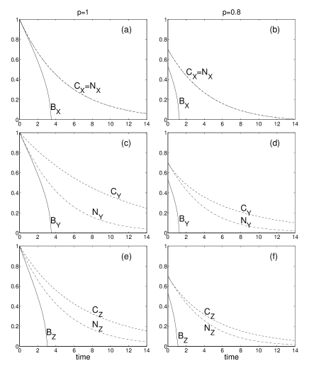
Figure 1: Decays of different measures for a given initial state in each sub-figure: The Bell-inequality violation degree $B_{\psi}^{(p)}(t)$, concurrence $C_{\psi}^{(p)}(t)$ and negativity $N_{\psi}^{(p)}(t)$ for qubits initially in the Werner states $\rho_{\psi}^{(p)}(0)$, where $\psi=X,Y,Z$ and $p=1$ (left panel) or $p=0.8$ (right panel), coupled to the same reservoir with the damping constant $\gamma_{1}=\gamma_{2}=0.1$.

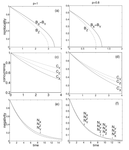
Figure 2: Decays of a given measure for different states in each sub-figure. Notation and parameters are the same as in figure 1.

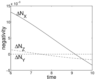
Figure 3: Negativities $\Delta N_{\psi}^{(p)}(t)=N_{\psi}^{(p)}(t)-N_{Y}^{(p)}(t)$ ($\psi=X,Y,Z$) corresponding to those presented in Fig. 2(f) and Table I for the same $\gamma_{1}=\gamma_{2}=0.1$ and $p=0.8$.

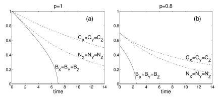
Figure 4: Same as in figure 1 but for one qubit coupled to the reservoir with the damping constant $\gamma_{1}=0.1$, and the second qubit undamped ($\gamma_{2}=0$).

IV Entanglement

To study the entanglement, we apply the concurrence and negativity being related to the entanglement of formation and entanglement cost, respectively.

The entanglement of formation of a mixed state $\rho$ is the minimum mean entanglement of an ensemble of pure states $|\psi_{i}\rangle$ that represents $\rho$ bennett2 :

$$E_{F}({\rho})=\min_{\{p_{i},|\psi_{i}\rangle\}}\sum_{i}p_{i}E(|\psi_{i}\rangle\langle\psi_{i}|)$$ (26)

where $\rho=\sum_{i}p_{i}|\psi_{i}\rangle\langle\psi_{i}|$ and $E(|\psi_{i}\rangle\langle\psi_{i}|)$ is the entropy of entanglement of pure state $|\psi_{i}\rangle$ defined by the von Neumann entropy. As shown by Wootters wootters , the entanglement of formation for two qubits in an arbitrary mixed state ${\rho}$ can explicitly be given as

$$E_{F}({\rho})=H\left(\textstyle{\frac{1}{2}}[1+\sqrt{1-C({\rho})^{2}}]\right)$$ (27)

where $H(x)$ is the binary entropy and $C({\rho})$ is the Wootters concurrence defined by

$$C({\rho})=\max\{0,2\max_{i}\lambda_{i}-\sum_{i=1}^{4}\lambda_{i}\}$$ (28)

where $\lambda_{i}$ are the square roots of the eigenvalues of the matrix ${\rho}({\sigma}_{y}\otimes{\sigma}_{y}){\rho}^{\ast}({\sigma}_{y}\otimes{\sigma}_{y})$, where ${\sigma}_{y}$ is the Pauli spin matrix and the asterisk denotes complex conjugation. $E_{F}(\rho)$ and $C(\rho)$ are monotonic functions of one another and both range from 0 (for a separable state) to 1 (for a maximally entangled state), so that “one can take the concurrence as a measure of entanglement in its own right” wootters .

The negativity is another measure of bipartite entanglement being related to the Peres-Horodecki criterion peres ; horodecki and defined by zyczkowski ; eisert ; vidal

$${N}({\rho})=\max\{0,-2\sum_{j}\mu_{j}\}$$ (29)

where ${\rho\equiv\rho}_{AB}$ is the density matrix of two subsystems (say, $A$ and $B$ with $d_{A}$ and $d_{B}$ levels, respectively), and the sum is taken over the negative eigenvalues $\mu_{j}$ of the partial transpose ${\rho}^{T_{A}}$ of ${\rho}$ with respect to one of subsystems (say $A$) in the basis $\{|0\rangle,|1\rangle,...,|d_{A}\rangle\}$:

$${\rho}^{T_{A}}=\sum_{i,j=0}^{d_{A}-1}\sum_{k,l=0}^{d_{B}-1}\langle i,k|\rho|j,l\rangle|j,k\rangle\langle i,l|.$$ (30)

For two-qubit ($d_{A}=d_{B}=2$) states, the sum in (29) can be skipped as ${\rho}^{T_{A}}$ has at most one negative eigenvalue sanpera . The negativity, especially in low-dimensional systems ($2\otimes 2$ and $2\otimes 3$), is a useful measure of entanglement satisfying the standard conditions eisert1 ; vidal . The negativity (29) ranges from 0 (for a separable state) to 1 (for a MES) similarly to the concurrence and the BIV degree. It is worth noting that the logarithmic negativity, $\log_{2}[{N}({\rho})+1]$, has a simple operational interpretation as a measure of the entanglement cost for the exact preparation of a two-qubit state $\rho$ under quantum operations preserving the positivity of the partial transpose (PPT) audenaert ; ishizaka04 .

The concurrences and negativities for all the three initial Werner states ${\rho}_{\psi}^{(p)}(0)$ ($\psi=X,Y,Z$) are the same and equal to

$$C_{\psi}^{(p)}(0)={N}_{\psi}^{(p)}(0)=\max\{0,\tfrac{1}{2}(3p-1)\}$$ (31)

but different from their BIV degree $B_{\psi}^{(p)}(0)$, given by (13). For the Bell states, all the entanglement measures and the BIV degree are equal to one. However, by decreasing parameter $p$, the BIV degree of the Werner states decreases faster than their entanglement. For example of $p=0.8$, the initial values of the concurrences and negativities are equal to 0.7 while the BIV degree is 0.529 as shown in the right panels of Figs. 1, 2, and 4. By comparing (13) and (31) it is seen that the Werner states are entangled iff $1/3<p\leq 1$. Thus, the Werner states for $p\in(1/3,1/\sqrt{2}\rangle$ are entangled although admitting a local hidden model, i.e., satisfying the Bell inequality werner .

Qubits initially in the Werner state ${\rho}_{X}^{(p)}(0)$ coupled to the thermal reservoirs exhibit dissipation described by (14). We find with the help of the Wootters formula that the concurrence for ${\rho}_{X}^{(p)}(t)$ exhibits the following decay

$$C_{X}^{(p)}(t)=\max\{0,\frac{\sqrt{g_{1}g_{2}}}{2}\left(2p-\sqrt{(2-qg_{1})(2-qg_{2})}\right)\}$$ (32)

with $q=1+p$. While the negativity, according to Peres-Horodecki criterion applied for ${\rho}_{X}^{(p)}(t)$, decays as

$$N_{X}^{(p)}(t) = \max\{0,\frac{1}{2}[-g_{1}-g_{2}+(1+p)g_{1}g_{2}$$ (33)

$$\qquad\qquad+\sqrt{(g_{1}-g_{2})^{2}+4p^{2}g_{1}g_{2}}]\}.$$

By assuming that both qubits are coupled to the same reservoir described the damping constant $\gamma\equiv\gamma_{1}=\gamma_{2}$, we observe that the concurrence and negativity are the same for all evolution times as described by

$$C_{X}^{(p)}(t)={N}_{X}^{(p)}(t)=\max\{0,\frac{g}{2}[(1+p)g-2(1-p)]\},$$ (34)

where $g=\exp(-\gamma t)$, as clearly depicted in Fig. 1(a,b). In another special case, for the initial Bell states ($p=1)$, the solutions for the concurrence and negativity simplify to

$$C_{X}^{(1)}(t) = \sqrt{g_{1}g_{2}}\left(1-\sqrt{(1-g_{1})(1-g_{2})}\right),$$

$${N}_{X}^{(1)}(t) = g_{1}g_{2},$$ (35)

respectively.

On the other hand, for qubits decaying from the initial Werner state ${\rho}_{Y}^{(p)}(0)$, as described by (16), the concurrence decays in time as

$$C_{Y}^{(p)}(t) = \max\{0,\frac{1}{2}\sqrt{g_{1}g_{2}}(2p-\sqrt{1-p}$$ (36)

$$\qquad\times\sqrt{(2-g_{1})(2-g_{2})-pg_{1}g_{2}})\}$$

while the negativity vanishes as follows

$$N_{Y}^{(p)}(t) = \max\{0,\frac{1}{2}(-2+g_{1}+g_{2}-(1-p)g_{1}g_{2}$$ (37)

$$+\sqrt{(2-g_{1}-g_{2})^{2}+4p^{2}g_{1}g_{2}})\}.$$

Note that decays of all the entanglement measures, similarly to the BIV degree, are independent of the sign in definitions of $|X\rangle$ and $|Y\rangle$. In a special case for qubits coupled to the same reservoir ($\gamma_{1}=\gamma_{2}$), (36) and (37) simplify, respectively, to

$$C_{Y}^{(p)}(t) = \max\{0,g\left(p-\sqrt{r(1-g)+\tfrac{1}{4}r^{2}g^{2}}\right)\},$$ (38)

$$N_{Y}^{(p)}(t) = \max\{0,\sqrt{(1-g)^{2}+p^{2}g^{2}}-\tfrac{1}{2}rg^{2}-(1-g)\}$$

with $r=1-p$. In another special case for the initial Bell state ($p=1$), the entanglement measures (36) and (37) reduce to

$$C_{Y}^{(1)}(t) = \sqrt{g_{1}g_{2}},$$ (39)

$$N_{Y}^{(1)}(t) = \frac{1}{2}\left(\sqrt{(2-g_{1}-g_{2})^{2}+4g_{1}g_{2}}+g_{1}+g_{2}-2\right),$$

respectively. It is worth mentioning that, in contrast to $C_{X}^{(p)}(t)={N}_{X}^{(p)}(t)$ for $\gamma_{1}=\gamma_{2},$ the evolutions $C_{Y}^{(p)}(t)$ and ${N}_{Y}^{(p)}(t)$ are different. Finally, let us briefly discuss the effect of dissipation of the initial Werner state ${\rho}_{Z}^{(p)}(0)$, described by (20), on the entangled measures. The general analytical formulas for the $p$-dependent concurrence and negativity are quite lengthy thus are not presented here explicitly although were used for plotting the corresponding curves in Figs. 1(e,f), 2(e,f) and 3. However, in a special case for the initial Bell-like state ($p=1$) the decays of the entanglement measures are simply given by:

$$C_{Z}^{(1)}(t) = \sqrt{g_{1}g_{2}}\left(1-\tfrac{1}{2}\sqrt{(1-g_{1})(1-g_{2})}\right),$$ (40)

$${N}_{Z}^{(1)}(t) = \tfrac{1}{2}\sqrt{g_{1}g_{2}(5+g_{1}g_{2}-2G)+4(1-G)^{2}}+G-1$$

with $G=(g_{1}+g_{2})/2$. By assuming the same damping constants $\gamma_{1}=\gamma_{2}$, e.g., the concurrence formula reduces to $C_{Z}^{(1)}(t)=g(1+g)/2$. A graphical comparison of the decays of all the measures is shown in Fig. 2 and of the negativities in Fig. 3 and Table I for $\gamma_{1}=\gamma_{2}=0.1$. Since the differences between the negativities $N_{\psi}^{(p)}(t)$ are not clear enough in Fig. 2(f), the curves were redrawn in Fig. 3 for the rescaled negativities $\Delta N_{\psi}^{(p)}(t)\equiv N_{\psi}^{(p)}(t)-N_{Y}^{(p)}(t)$ with $\psi=X,Y,Z$.

For clear analysis of the entanglement measures we will now focus on the special case for $p=1$. A comparison of Eqs. (35), (39), and (40) implies that the following inequalities are satisfied

$$C_{Y}^{(1)}(t)\geq C_{Z}^{(1)}(t)\geq C_{X}^{(1)}(t)$$ (41)

for any evolution times. In the short time approximation, we find that the concurrences for $\rho^{(1)}_{\psi}$ ($\psi=X,Y,Z$) decay up to linear terms in time as follows

$$C_{\psi}^{(1)}(t) = 1-\frac{1}{2}(\gamma_{1}+\gamma_{2}+f_{\psi}\sqrt{\gamma_{1}\gamma_{2}})t+{\mathcal{O}}(t^{2})$$ (42)

where $f_{X}=2$, $f_{Y}=0$, and $f_{Z}=1$, which confirms the validity of (41). Contrary to the concurrences, the negativities in the short-time limit decay as follows

$$N_{\psi}^{(1)}(t)=1-(\gamma_{1}+\gamma_{2})t+\frac{1}{2}(\gamma_{1}^{2}+f^{\prime}_{\psi}\gamma_{1}\gamma_{2}+\gamma_{2}^{2})t^{2}+{\mathcal{O}}(t^{3})$$ (43)

where $f^{\prime}_{X}=2$, $f^{\prime}_{Y}=1$, and $f^{\prime}_{Z}=5/4$, which implies that at short evolution times the inequalities hold

$$N_{X}^{(1)}(t)\geq N_{Z}^{(1)}(t)\geq N_{Y}^{(1)}(t).$$ (44)

A closer look at the inequalities (24), (41) and (44) enables us to conclude that there exist states of two qubits (e.g., $\rho_{X}^{(1)}(t)$ and $\rho_{Y}^{(1)}(t)$ at some short evolution time t) exhibiting the same BIV degree, $B_{X}^{(1)}(t)=B_{Y}^{(1)}(t)$, but different entanglement measures in such a way that the concurrence $C_{X}^{(1)}(t)$ is smaller than $C_{Y}^{(1)}(t)$, while the negativity $N_{X}^{(1)}(t)$ is greater than $N_{Y}^{(1)}(t)$. Obviously, the inequalities (41) for the concurrences correspond to those for the entanglement of formation, while the inequalities (44) for the negativities correspond to those for the PPT-entanglement cost. We stress that for longer times inequalities different from (44) are satisfied for $p<1$ as presented in Table I. By analyzing this Table, other states differently ordered by the entanglement measures are readily recognized, including those at time $t=t_{2}$, for which $B_{X}^{(.8)}(t)=B_{Y}^{(.8)}(t)$, $N_{X}^{(.8)}(t)=N_{Y}^{(.8)}(t)$ but $C_{X}^{(.8)}(t)<C_{Y}^{(.8)}(t)$.

By comparing the series expansions (42) and (43) for $\gamma_{1},\gamma_{2}>0$, we can conclude that all the three negativities evolve in a more similar way (precisely they are the same up to linear terms in time) in comparison to more distinct evolutions of the corresponding concurrences. Also by analyzing (22) and (43) for $p=1$, one observes that the negativities $N_{X,Y,Z}^{(1)}(t)$ and the BIV degrees $B_{X,Y}^{(1)}(t)$ decay in the same manner up to linear terms in time for arbitrary values of $\gamma_{1}$ and $\gamma_{2}$. Other similarities of the decays of the entanglement and/or the BIV degree can be found for some special choices of the damping constants. In particular, (34) is valid for $\gamma_{1}=\gamma_{2}$. In another special case of only one of the qubits coupled to the reservoir, e.g. $\gamma_{1}\neq 0$ and $\gamma_{2}=0$, the BIV degrees of all the three states decrease, as given by (25), but also the entanglement measures decrease at the same rate as expressed by their concurrence

$$C_{X}^{(p)}(\gamma_{2}=0,t)=C_{Y}^{(p)}(\gamma_{2}=0,t)=C_{Z}^{(p)}(\gamma_{2}=0,t)$$

$$=\max\{0,\frac{1}{2}\sqrt{g_{1}}\left(2p-\sqrt{(1-p)[2-(1+p)g_{1}]}\right)\}$$ (45)

and negativity

$$N_{X}^{(p)}(\gamma_{2}=0,t)=N_{Y}^{(p)}(\gamma_{2}=0,t)=N_{Z}^{(p)}(\gamma_{2}=0,t)$$

$$=\max\{0,\frac{1}{2}\left(pg_{1}+\sqrt{(1-g_{1})^{2}+4p^{2}g_{1}}-1\right)\}.$$ (46)

By restricting to the case of the initial MESs ($p=1$), the above equations reduce to ($\psi=X,Y,Z$):

$$C_{\psi}^{(1)}(\gamma_{2}=0,t)=\sqrt{g_{1}},$$

$$N_{\psi}^{(1)}(\gamma_{2}=0,t)=g_{1}.$$ (47)

These conclusions are confirmed numerically on the examples of $\gamma_{1}=0.1$, $p=0.8$ and $p=1$ as shown in Fig. 4.

Table 1: Comparison of the negativities for the three initial Werner states for $p=0.8$, $\gamma_{1}=\gamma_{2}=0.1$ as in Figs. 2(f) and 3. The characteristic evolution times are $t_{1}\approx 7.4745$, $t_{2}\approx 9.1613$, $t_{3}\approx 9.5209$. The corresponding inequalities for the BIV degrees are $B_{X}^{(p)}(t)=B_{Y}^{(p)}(t)\geq B_{Z}^{(p)}(t)$, and for the concurrences are $C_{Y}^{(p)}(t)\geq C_{Z}^{(p)}(t)\geq C_{X}^{(p)}(t)$.

time	negativities
$t\in(0,t_{1})$	$N_{X}^{(p)}(t)>N_{Z}^{(p)}(t)>N_{Y}^{(p)}(t)$
$t=t_{1}$	$N_{X}^{(p)}(t)>N_{Y}^{(p)}(t)=N_{Z}^{(p)}(t)$
$t\in(t_{1},t_{2})$	$N_{X}^{(p)}(t)>N_{Y}^{(p)}(t)>N_{Z}^{(p)}(t)$
$t=t_{2}$	$N_{X}^{(p)}(t)=N_{Y}^{(p)}(t)>N_{Z}^{(p)}(t)$
$t\in(t_{2},t_{3})$	$N_{Y}^{(p)}(t)>N_{X}^{(p)}(t)>N_{Z}^{(p)}(t)$
$t=t_{3}$	$N_{Y}^{(p)}(t)>N_{X}^{(p)}(t)=N_{Z}^{(p)}(t)$
$t\in(t_{3},100)$	$N_{Y}^{(p)}(t)>N_{Z}^{(p)}(t)>N_{X}^{(p)}(t)$

V Conclusions

We have analyzed quantum-information properties of two decaying optical qubits prepared initially in Werner or Werner-like states and coupled to thermal reservoirs within the master equation approach. We have studied in detail a degree of violation of the Bell inequality due to Clauser, Horne, Shimony and Holt clauser by applying a parameter $B$ related to the maximum possible mean value of the Bell operator in a given state according to the Horodecki criterion horodecki1 . On the other hand, the degree of the entanglement was expressed by the Wootters concurrence $C$ wootters , as a measure of the entanglement of formation, and by the negativity $N$ based on the Peres-Horodecki criterion peres ; horodecki and related to the PPT-entanglement cost audenaert . We have observed, as manifestations of the symmetry of our particular decoherence mechanism, the following properties of the decaying Werner states in relation to the Bell-inequality violation degree $B$ and the entanglement measures $C$ and $N$: If only one qubit is coupled to the thermal reservoir than those decays are independent of the initial Werner or Werner-like state for a given $p$. However, if both qubits are coupled to the reservoir(s) then the decays of $C$ and $N$, and in some cases $B$, depend on the initial Werner or Werner-like state. By analyzing these decays, we have found states (say $\rho$ and $\sigma$) of two qubits exhibiting the same degree the Bell-inequality violation, $B_{\rho}=B_{\sigma}$, but different entanglement measures in such a way that the concurrence $C_{\rho}$ is smaller than $C_{\sigma}$, while the negativity $N_{\rho}$ is greater than $N_{\sigma}$. We have also found other states $\rho$ and $\sigma$, for which either (i) $B_{\rho}=B_{\sigma}$, $C_{\rho}<C_{\sigma}$ and $N_{\rho}<N_{\sigma}$, or (ii) $B_{\rho}=B_{\sigma}$, $N_{\rho}=N_{\sigma}$ and $C_{\rho}<C_{\sigma}$. Thus, the analysis of the decaying Werner states shows clearly the relativity of two-qubit entanglement measures.

References

- (1) J. S. Bell, Physics (Lon Island City, N.Y.) 1, 195 (1964).
- (2) J. F. Clauser, M. A. Horne, A. Shimony, R. A. Holt, Phys. Rev. Lett. 23, 880 (1969).
- (3) W. Tittel, G. Weihs, Quantum Inform. Comp. 1, 3 (2001).
- (4) N. Gisin, Phys. Lett. A 154, 201 (1991).
- (5) R. F. Werner, Phys. Rev. A 40, 4277 (1989).
- (6) W. J. Munro, D. F. V. James, A. G. White, P. G. Kwiat, Phys. Rev. A 64, 030302(R) (2001).
- (7) S. Ghosh, G. Kar, A. Sen De, U. Sen, Phys. Rev. A 64, 044301 (2001).
- (8) T. C. Wei, K. Nemoto, P. M. Goldbart, P. G. Kwiat, W. J. Munro, F. Verstraete, Phys. Rev. A 67, 022110 (2003).
- (9) S. Popescu, Phys. Rev. Lett. 72, 797 (1994).
- (10) J. Lee, M. S. Kim, Phys. Rev. Lett. 84, 4236 (2000).
- (11) S. Ishizaka, T. Hiroshima, Phys. Rev. A 62, 022310 (2000).
- (12) J. Eisert, M. Plenio, J. Mod. Opt. 46, 145 (1999).
- (13) S. Virmani, M. B. Plenio, Phys. Lett. A 268, 31 (2000).
- (14) K. Życzkowski, Phys. Rev. A 60, 3496 (1999).
- (15) F. Verstraete, K. M. R. Audenaert, J. Dehaene, B. De Moor, J. Phys. A 34, 10327 (2001).
- (16) K. Życzkowski, I. Bengtsson, Ann. Phys. (N.Y.) 295, 115 (2002).
- (17) T. C. Wei, P. M. Goldbart, Phys. Rev. A 68, 042307 (2003).
- (18) V. Giovannetti, D. Vitali, P. Tombesi, A. K. Ekert, Phys. Rev. A 62, 032306 (2000).
- (19) R. Horodecki, P. Horodecki, M. Horodecki, Phys. Lett. A 200, 340 (1995)
- (20) R. Horodecki, Phys. Lett. A 210, 223 (1996).
- (21) M. Jakob, Y. Abranyos, J. A. Bergou, Phys. Rev. A 66, 022113 (2002).
- (22) L. Jakóbczyk, A. Jamróz, Phys. Lett. A 318, 318 (203).
- (23) C. H. Bennett, D. P. DiVincenzo, J. A. Smolin, W. K. Wootters, Phys. Rev. A 54, 3824 (1996).
- (24) W. K. Wootters, Phys. Rev. Lett. 80, 2245 (1998).
- (25) A. Peres, Phys. Rev. Lett. 77, 1413 (1996).
- (26) M. Horodecki, P. Horodecki, R. Horodecki, Phys. Lett. A 223, 1 (1996).
- (27) K. Życzkowski, P. Horodecki, A. Sanpera, M. Lewenstein, Phys. Rev. A 58 883 (1998).
- (28) J. Eisert, Ph.D. Thesis (University of Potsdam) (2001).
- (29) G. Vidal, R. F Werner, Phys. Rev. A 65, 032314 (2002).
- (30) A. Sanpera, R. Tarrach, G. Vidal, Phys. Rev. A 58, 826 (1998).
- (31) K. Audenaert, M. B. Plenio, J. Eisert, Phys. Rev. Lett. 90, 27901 (2003).
- (32) S. Ishizaka, Phys. Rev. A 69, 020301 (2004).