Post-processing with linear optics for improving the quality of single-photon sources

Abstract

Triggered single-photon sources produce the vacuum state with non-negligible probability, but produce a much smaller multiphoton component. It is therefore reasonable to approximate the output of these photon sources as a mixture of the vacuum and single-photon states. We show that it is impossible to increase the probability for a single photon using linear optics and photodetection on fewer than four modes. This impossibility is due to the incoherence of the inputs; if the inputs were pure-state superpositions, it would be possible to obtain a perfect single-photon output. In the more general case, a chain of beam splitters can be used to increase the probability for a single photon, but at the expense of adding an additional multiphoton component. This improvement is robust against detector inefficiencies, but is degraded by dark counts or multiphoton components in the input.

I Introduction

One of the most promising methods for quantum information processing is linear optics and photodetection. Linear optics and photodetection may be used for provably secure quantum communication BB84 , as well as quantum computation LOQC . An important requirement for these schemes is the ability to produce a single photon on demand key ; LOQC , yet generating high-fidelity single-photon states is challenging. The traditional method for generating single photons involves photodetection on one output mode from a non-degenerate parametric down-conversion process to post-select a single photon in the correlated mode down ; fid . This method has the drawback that the time of the photon emission is not controlled. More recently, triggered photon sources have been developed, including molecules mol , quantum wells well , colour centers col , ions ion and quantum dots dot . These sources have a significant vacuum contribution, but the multiphoton contribution may be made very small twophot .

For the majority of this study, we approximate these sources by taking the multiphoton probability to be zero. That is, we consider an idealised single-mode single-photon source, which may be represented by the density operator

$$\hat{\rho}_{p}=(1-p)|{0}\rangle\langle{0}|+p|{1}\rangle\langle{1}|.$$ (1)

Here $p$ is the probability for a single photon, and is also called the efficiency. Increasing the efficiency is important because many quantum optics experiments, especially those concerned with linear optical quantum computation, require high efficiency sources. We also derive results for states with a coherent superposition of the vacuum and a single photon; however, this form of state is not produced by single-photon sources.

Much effort is directed towards improving sources, but here we pose the question as to whether it is possible to perform post-processing to obtain higher efficiency. Ideally this post-processing should also maintain a zero multiphoton contribution (though a very small multiphoton contribution would also be acceptable). A promising method of post-processing is linear optics and photodetection. As mentioned above, linear optics and photodetection can be used to perform quantum computation LOQC , and optical controlled-NOT gates have recently been demonstrated CNOT ; however, there are also no-go theorems for linear optics nogo .

In a recent publication BSSK we investigated the possibility of improving the single-photon efficiency $p$ with linear optical elements and photodetection. Here we present a number of new results that clarify the limitations inherent in this method, as well as reviewing the results presented in BSSK . In particular, we analyse the effects of various experimental limitations, present a scheme that gives perfect results for inputs with a coherent superposition of zero and one photon, and show connections between some difficult unsolved problems.

We begin by showing that it is not possible to obtain an improvement for the simple case of a beam splitter in Sec. II. In Sec. III we show that, if we allow a coherent superposition of zero and one photon, rather than an incoherent mixture, it is possible to obtain a perfect single-photon state. We then proceed to the case of a multimode interferometer with incoherent inputs in Sec. IV. In Secs. V and VI we give an expanded discussion of the limit on the improvement that it is possible to obtain, and the method to obtain an improvement. Sec. VII gives a detailed discussion of the impact of various experimental problems on this method. We give further discussion of no-go theorems for post-processing in Sec. VIII. Then, in Sec. IX, we show that there are deep connections between the unsolved problems for post-processing. Lastly we give a discussion of how the theory is changed by allowing multiphoton contributions in the inputs in Sec. X, and we conclude in Sec. XI.

II Beam splitter

To begin, we consider the simplest case of two copies of the quantum state (1) combined on a single beam splitter. The initial state can be written in the form

$$\hat{\rho}_{\text{in}}^{(2)}=(1-p_{1})(1-p_{2})|{00}\rangle\langle{00}|+p_{1}(1-p_{2})|{10}\rangle\langle{10}|+p_{2}(1-p_{1})|{01}\rangle\langle{01}|+p_{1}p_{2}|{11}\rangle\langle{11}|.$$ (2)

Each photonic mode operator gets transformed by the beam splitter in the following way:

$$\hat{a}_{1}^{\dagger}\mapsto\Lambda_{11}\hat{a}_{1}^{\dagger}+\Lambda_{21}\hat{a}_{2}^{\dagger},\qquad\hat{a}_{2}^{\dagger}\mapsto\Lambda_{12}\hat{a}_{1}^{\dagger}+\Lambda_{22}\hat{a}_{2}^{\dagger},$$ (3)

where $\bm{\Lambda}$ is a $2\times 2$ unitary matrix VogelWelsch . We have two options, to project onto the vacuum or onto the single-photon Fock state (projecting onto two photons results in vacuum output in the unmeasured mode). After vacuum projection in mode 2, we end up with an unnormalised state of the form

$$\hat{\rho}_{\text{out}}^{(2)}\propto|{0}\rangle\langle{0}|+\left(\frac{p_{1}}{1-p_{1}}|\Lambda_{11}|^{2}+\frac{p_{2}}{1-p_{2}}|\Lambda_{12}|^{2}\right)|{1}\rangle\langle{1}|+\text{2-photon term}.$$ (4)

Thus the ratio between the probabilities for one and zero photons is just a weighted average of $p_{1}/(1-p_{1})$ and $p_{2}/(1-p_{2})$, and cannot exceed either of these. That is, it is not possible to improve the ratio between the probabilities for obtaining one and zero photons. This automatically implies that it is not possible to improve the absolute probability of obtaining one photon.

In the case of a single-photon detection, the resulting unnormalised state is

$$\hat{\rho}_{\text{out}}^{(2)}\propto\left(\frac{1-p_{1}}{p_{1}}|\Lambda_{22}|^{2}+\frac{1-p_{2}}{p_{2}}|\Lambda_{21}|^{2}\right)|{0}\rangle\langle{0}|+|\text{per}\bm{\Lambda}|^{2}|{1}\rangle\langle{1}|,$$ (5)

where $\text{per}\bm{\Lambda}$ is the permanent perm of the beam splitter matrix $\bm{\Lambda}$. Since the absolute value of the permanent of a unitary matrix is bounded from above by unity, and the term in brackets is a weighted sum of terms $(1-p_{i})/p_{i}$, we do not find any improvement for this case either. Hence there is no improvement in the probability for a single photon if zero, one or two photons are detected. These results demonstrate that for mixed-state inputs it is impossible to obtain an improvement in the single-photon probability using a beam splitter.

III Pure-state inputs

It is possible to obtain an improvement using a beam splitter if the inputs are in pure-state superpositions of zero and one photon, instead of incoherent mixtures. Consider two input modes that are each in the state $\alpha|{0}\rangle+\beta|{1}\rangle$. The initial state may be written as

$$|{\psi}\rangle_{\text{in}}^{(2)}=\left[\alpha^{2}+\alpha\beta(a_{1}^{\dagger}+a_{2}^{\dagger})+\beta^{2}a_{1}^{\dagger}a_{2}^{\dagger}\right]|{00}\rangle.$$ (6)

Applying the beam splitter transformation (3) gives

$$|{\psi}\rangle_{\text{trans}}^{(2)}=\left\{\alpha^{2}+\alpha\beta\left[(\Lambda_{11}+\Lambda_{12})a_{1}^{\dagger}+(\Lambda_{21}+\Lambda_{22})a_{2}^{\dagger}\right]+\beta^{2}\left[\Lambda_{11}\Lambda_{12}(a_{1}^{\dagger})^{2}+\Lambda_{21}\Lambda_{22}(a_{2}^{\dagger})^{2}+(\text{per}\bm{\Lambda})a_{1}^{\dagger}a_{2}^{\dagger}\right]\right\}|{00}\rangle.$$ (7)

Conditioning on detection of zero photons in mode 2 gives the output state

$$|{\psi}\rangle_{\text{out}}^{(2)}\propto\alpha^{2}|{0}\rangle+\alpha\beta(\Lambda_{11}+\Lambda_{12})|{1}\rangle+\sqrt{2}\beta^{2}\Lambda_{11}\Lambda_{12}|{2}\rangle.$$ (8)

It is easily seen that this output state may have a higher probability for a single photon. For example, if the initial state is close to the vacuum state (i.e. $\alpha\gg\beta$), then an improvement by a factor of two may be obtained by using $\Lambda_{11}=\Lambda_{12}=1/\sqrt{2}$.

In fact, it is possible to further process this output state to obtain a perfect single-photon state. If we combine this state with mode 3, which is also assumed to be prepared in state $\alpha|{0}\rangle+\beta|{1}\rangle$, then the total state may be represented as

$$|{\psi}\rangle_{\text{in}}^{(3)}\propto\left[\alpha^{2}+\alpha\beta(\Lambda_{11}+\Lambda_{12})a_{1}^{\dagger}+\beta^{2}\Lambda_{11}\Lambda_{12}(a_{1}^{\dagger})^{2}\right]\left(\alpha+\beta a_{3}^{\dagger}\right)|{00}\rangle.$$ (9)

Applying the beam splitter transformation (3) (except using a prime to distinguish this beam splitter from the previous one) gives

$$|{\psi}\rangle_{\text{trans}}^{(3)}\propto\left[\alpha^{2}+\alpha\beta(\Lambda_{11}+\Lambda_{12})(\Lambda^{\prime}_{11}\hat{a}_{1}^{\dagger}+\Lambda^{\prime}_{31}\hat{a}_{3}^{\dagger})+\beta^{2}\Lambda_{11}\Lambda_{12}(\Lambda^{\prime}_{11}\hat{a}_{1}^{\dagger}+\Lambda^{\prime}_{31}\hat{a}_{3}^{\dagger})^{2}\right]\left[\alpha+\beta(\Lambda^{\prime}_{13}\hat{a}_{1}^{\dagger}+\Lambda^{\prime}_{33}\hat{a}_{3}^{\dagger})\right]|{00}\rangle.$$ (10)

Conditioning on detection of two photons gives

$$|{\psi}\rangle_{\text{out}}^{(3)}\propto\sqrt{2}\beta^{2}\Lambda^{\prime}_{31}\left\{\alpha\left[(\Lambda_{11}+\Lambda_{12})\Lambda^{\prime}_{33}+\Lambda_{11}\Lambda_{12}\Lambda^{\prime}_{31}\right]|{0}\rangle+\beta\Lambda_{11}\Lambda_{12}\left(2\Lambda^{\prime}_{11}\Lambda^{\prime}_{33}+\Lambda^{\prime}_{31}\Lambda^{\prime}_{13}\right)|{1}\rangle\right\}$$ (11)

To make this equation more clear, we use

$$\bm{\Lambda}=\left[\begin{array}[]{*{20}c}e^{i\phi}\cos{\theta}&-\sin{\theta}\\ \sin\theta&e^{-i\phi}\cos\theta\\ \end{array}\right],\qquad\bm{\Lambda}^{\prime}=\left[\begin{array}[]{*{20}c}e^{i\phi^{\prime}}\cos\theta^{\prime}&-\sin\theta^{\prime}\\ \sin\theta^{\prime}&e^{-i\phi^{\prime}}\cos\theta^{\prime}\\ \end{array}\right].$$ (12)

The condition that the output state is a pure single-photon state then becomes

$$(\cos\theta-e^{-i\phi}\sin\theta)e^{-i\phi^{\prime}}\cos\theta^{\prime}-\sin\theta\cos\theta\sin\theta^{\prime}=0.$$ (13)

This equation may be satisfied by taking $\theta^{\prime}$ and $\phi^{\prime}$ to be

$$\theta^{\prime}=\arctan\left(\frac{|\cos\theta-e^{-i\phi}\sin\theta|}{\sin\theta\cos\theta}\right),\qquad\phi^{\prime}=\arg(\cos\theta-e^{-i\phi}\sin\theta).$$ (14)

That is, regardless of the characteristics of the initial beam splitter (provided $\sin\theta$ and $\cos\theta$ are nonzero), it is possible to obtain a perfect single-photon output.

Another issue is the probability for obtaining the desired pattern of detection results. Using the unnormalised expression for $|{\psi}\rangle_{\text{out}}^{(3)}$ above, this probability is given by

$$P =2|\beta|^{6}\sin^{2}\theta\cos^{2}\theta\sin^{2}\theta^{\prime}(2\cos^{2}\theta^{\prime}-\sin^{2}\theta^{\prime})^{2}$$

$$=|\beta|^{6}\frac{\frac{1}{2}\sin^{2}2\theta(1-\cos\phi\sin 2\theta)\left(\frac{1}{2}\sin^{2}2\theta-1+\cos\phi\sin 2\theta\right)^{2}}{\left(\frac{1}{4}\sin^{2}2\theta+1-\cos\phi\sin 2\theta\right)^{3}}.$$ (15)

In the second line we have used the expression (14) for $\theta^{\prime}$. This probability is plotted in Fig. 1 for the range $0$ to $\pi$ in $\theta$ and $\phi$ ($P$ is periodic with period $\pi$ in these variables). There are four maxima in this range, for $(\theta,\phi)=(\pi/4,\pi)$, $(\pi/4,\text{acos}(13/14))$, $(3\pi/4,0)$ and $(3\pi/4,\text{acos}(-13/14))$. The exact values of $\phi$ of $\text{acos}(13/14)$ and $\text{acos}(-13/14)$ are not obvious from the plot but are straightforward to obtain analytically. The two maxima $(\pi/4,\pi)$ and $(3\pi/4,0)$ correspond to the same beam splitter, so there are only three maxima that correspond to distinct beam splitters. Each of these maxima is exactly the same height,

$$P_{\text{max}}=16|\beta|^{6}/81.$$ (16)

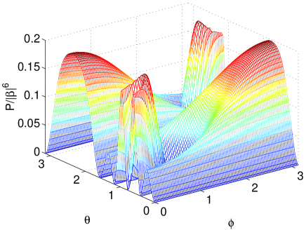
Figure 1: The probability of obtaining the desired detection results as a function of the beam splitter parameters $\theta$ and $\phi$ for the first beam splitter.

One factor that distinguishes the maxima is the sensitivity to the parameters. Clearly the maxima at $(\pi/4,\text{acos}(13/14))$ and $(3\pi/4,\text{acos}(-13/14))$ are far more sensitive to the values of $\theta$ and $\phi$, and it is therefore better to use the beam splitter corresponding to $(\pi/4,\pi)$ and $(3\pi/4,0)$. For the second beam splitter, the appropriate parameters are $\theta^{\prime}=\text{acos}(1/3)$ and $\phi^{\prime}=0$. That is, the best result is obtained by using a $50/50$ beam splitter followed by a beam splitter with a reflectivity of $1/9$.

Thus we see that, if the inputs to an interferometer are in pure superposition states, it is possible to obtain a perfect single-photon output for three modes. In contrast, if the inputs to the interferometer are incoherent superpositions of Fock states, it is impossible to obtain an improvement in the single-photon probability for three modes BSSK . These results imply that it is the incoherence in the inputs that prevents an improvement in the single photon probability. It would be interesting to determine the degree of decoherence that is sufficient to prevent an improvement in the single-photon efficiency. However, this is a difficult problem, which we leave to further investigation.

IV Multimode incoherent inputs

Although it is possible to obtain perfect single-photon states from pure superposition states, this method can not be applied to current experiments, as single-photon sources do not produce pure superposition states. Real single-photon sources produce an incoherent combination of Fock states; therefore we consider input states of this form for the remainder of this paper. In the multimode case we start with a supply of $N$ mixed states of the form (1). For additional generality we allow the different inputs to have different probabilities for a single photon, $p_{i}$, and we denote the maximum of these probabilities by $p_{\rm max}$. The initial input state may be described by

$$\hat{\rho}_{\text{in}}^{(N)} =\bigotimes_{i=1}^{N}\big{[}(1-p_{i})|{0}\rangle\langle{0}|+p_{i}|{1}\rangle\langle{1}|\big{]}$$

$$=\sum_{\bm{s}}P_{\bm{s}}\left(\prod_{i}(\hat{a}_{i}^{\dagger})^{s_{i}}|{0}\rangle\langle{0}|\prod_{i}(\hat{a}_{i})^{s_{i}}\right),$$ (17)

where $P_{\bm{s}}=\prod_{i}p_{i}^{s_{i}}(1-p_{i})^{1-s_{i}}$, and the vector $\bm{s}$ $\!=$ $\!(s_{1},\cdots,s_{N})^{T}$, ($s_{i}=0,1$), gives the photon numbers in the inputs. The quantity $P_{\bm{s}}$ is the probability of obtaining this combination of input photon numbers.

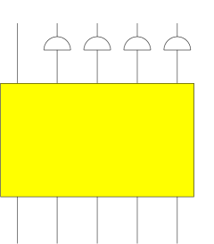
Figure 2: Schematic setup of the network. We assume $N$ incoming modes prepared in the state (IV) with different $p_{i}$. The photon number is measured in output modes 2 to $N$, and we wish to improve the probability for a single photon in mode 1.

This input is then passed through a passive interferometer which consists of beam splitters, mirrors, and phase shifters. Each of these elements preserves total photon number from input to output under ideal conditions. No energy is required to operate these optical elements, hence the term passive (also known as linear optical elements). More generally, polarisation transforming elements can be included, but here we are concerned only with a scalar field treatment; in fact polarisation effects could be included by doubling the number of channels and treating the two polarisations in a mode as two separate channels.

Classically the field amplitude of channel $i$ would be represented by the complex number $a_{i}$. The set of all field amplitudes for the $N$-channel interferometer is given by the vector $\bm{a}=(a_{1},\cdots,a_{N})^{\text{T}}$. The passive interferometer transforms the input amplitudes to the output amplitudes via the matrix transformation $\bm{a}\mapsto\bm{\Lambda}^{\dagger}\bm{a}$ with $\Lambda\in\text{U}(N)$, where U$(N)$ is the set of all $N\times N$ unitary matrices. Quantisation of the field is obtained by the replacement of $\bm{a}$ by the vector annihilation operator $\hat{\bm{a}}$, and the interferometer transforms the operators according to $\hat{\bm{a}}^{\dagger}\mapsto\bm{\Lambda}^{\rm T}\hat{\bm{a}}^{\dagger}$ VogelWelsch . This transformation of the operators yields

$$\hat{\rho}_{\rm trans}^{(N)}=\sum_{\bm{s}}P_{\bm{s}}\left[\prod_{i}\left(\sum_{k}\Lambda_{ki}\hat{a}_{k}^{\dagger}\right)^{s_{i}}|{0}\rangle\langle{0}|\prod_{i}\left(\sum_{k}\Lambda_{ki}^{*}\hat{a}_{k}\right)^{s_{i}}\right].$$ (18)

In the completely general case, we could perform photodetections on $N-N_{1}$ of the modes, and use the remaining $N_{1}$ modes as single-photon sources if the desired combination of detection results is obtained. However, this generality is not needed here because we are concerned with the maximum improvement in the photon statistics in a single mode. In order to fix notation, we denote as mode 1 that mode for which we want to improve the statistics, and label the other modes where photodetections have not been performed as modes 2 to $N_{1}$. The reduced density matrix in mode 1 is then identical to what would be obtained if photodetections were performed on modes 2 to $N_{1}$ (as well as $N_{1}+1$ to $N$), and the results of these photodetections discarded. Therefore, the probability for a single photon will be a weighted average of the single-photon probabilities for the different combinations of detections in modes 2 to $N_{1}$. Hence the maximum single-photon probability in mode 1 will be obtained for some combination of detections in modes 2 to $N_{1}$. For this reason we consider the state in mode 1 conditioned on photodetections in the other $N-1$ modes. As our aim is to determine the best results possible using linear optics and photodetection, we also assume that the photodetectors perform perfect photon counting measurements (imperfect detection is discussed later).

Before determining the conditional output state, we introduce some additional notation. The total number of photons detected is $D$, and the maximum possible number of photons input to the interferometer is $M$. As some of the $p_{i}$ may be equal to zero, $M$ may be less than $N$; $M$ is equal to the number of nonzero values of $p_{i}$. For $j>1$, $n_{j}$ is the number of photons detected in mode $j$, and $n_{1}$ is the photon number in mode 1 (the output mode). We use the notation $\Sigma_{n}=\sum_{i}n_{i}$ (so $\Sigma_{n}=D+n_{1}$) and $\Sigma_{s}=\sum_{i}s_{i}$. In addition, we define the set $\Phi_{\bm{s}}=\{i|s_{i}=1\}$, and let ${\rm Y}_{\bm{s}}$ be the set that consists of all vectors comprised of the elements of $\Phi_{\bm{s}}$.

The conditional state in mode 1 after photodetection in modes 2 to $N$ is

$$\hat{\rho}_{\rm out}^{(N)}=\sum_{n_{1}=0}^{N}c_{n_{1}}|{n_{1}}\rangle\langle{n_{1}}|.$$ (19)

Each coefficient $c_{n_{1}}$ is given by

$$c_{n_{1}}=K\langle{\bm{n}}|\hat{\rho}_{\rm trans}^{(N)}|{\bm{n}}\rangle,$$ (20)

where $|{\bm{n}}\rangle$ is a tensor product of number states in each of the output modes and the normalisation constant $K$ is equal to

$$K=\left[\sum_{n_{1}=0}^{N}\langle{\bm{n}}|\hat{\rho}_{\rm trans}^{(N)}|{\bm{n}}\rangle\right]^{-1}.$$ (21)

Evaluating $c_{n_{1}}$ gives

$$c_{n_{1}}=\frac{K^{\prime}}{n_{1}!}\sum_{\bm{s};\Sigma_{\bm{s}}=\Sigma_{\bm{n}}}P_{\bm{s}}\left|S_{\bm{s},\bm{n}}\right|^{2},$$ (22)

where $K^{\prime}=K/\prod_{j=2}^{N}n_{j}!$, and

$$S_{\bm{s},\bm{n}}=\sum_{\bm{\sigma}\in{\rm Y}_{\bm{s}}}\left(\Lambda_{1,\sigma_{1}}\cdots\Lambda_{1,\sigma_{n_{1}}}\right)\cdots\left(\Lambda_{N,\sigma_{\Sigma_{\bm{s}}-n_{N}+1}}\cdots\Lambda_{N,\sigma_{\Sigma_{\bm{s}}}}\right).$$ (23)

This quantity may alternatively be expressed using permanents as

$$S_{\bm{s},\bm{n}}=\text{per}(\bm{\Lambda}[\bm{n},\bm{s}]).$$ (24)

Here the notation $\bm{\Lambda}[\bm{n},\bm{s}]$ is used to indicate that the $i$’th column of $\bm{\Lambda}$ is repeated $s_{i}$ times, and the $j$’th row is repeated $n_{j}$ times.

Two figures of merit for an arbitrary single mode field $\sum_{i}q_{i}|{i}\rangle\langle{i}|$ are

$$R=\frac{q_{1}}{q_{0}},\qquad G=\frac{q_{2}/q_{1}}{q_{1}/q_{0}}.$$ (25)

We use the subscript “out” to indicate the output field, and “in” to indicate the input field. For the output field we simply have $q_{i}=c_{i}$. For the input field, we have $G_{\rm in}=0$, as the two-photon component is assumed be negligible. For simplicity we define $R_{\rm in}$ to be the maximum input ratio $p_{\rm max}/(1-p_{\rm max})$.

The figure of merit $G$ characterises the two-photon contribution, and is equal to $1/2$ for Poisson photon statistics. If the multiphoton component in the output is zero, then comparing $R_{\rm in}$ and $R_{\rm out}$ immediately tells us if there is an improvement in the probability for a single photon. Even if the multiphoton component is nonzero, using $R_{\rm out}$ has the advantages:
1. The common constant $K^{\prime}$ cancels, so it is possible to evaluate $R_{\rm out}$ analytically.
2. If $R_{\rm out}\leq R_{\rm in}$, then it is clear that $c_{1}\leq p_{\rm max}$. Thus we can determine those cases where there is no improvement.
3. For $p_{\rm max}\ll 1$, $c_{0}\approx 1$ and $R_{\rm in}\approx p_{\rm max}$. Therefore the improvement in $R$ is approximately the same as the improvement in the single-photon probability over $p_{\rm max}$.

An alternative measure of the multiphoton contributions is given by how sub-Poissonian the field is. That is, we may define the measure

$$\Pi=\frac{\langle\hat{n}^{2}\rangle-\langle\hat{n}\rangle^{2}}{\langle\hat{n}\rangle}.$$ (26)

For a sub-Poissonian field, $\Pi<1$. States of the form (1) are sub-Poissonian, with $\Pi=1-p$. We take $\Pi_{\rm in}$ to be the minimum value in the inputs, $1-p_{\rm max}$, and $\Pi_{\rm out}$ is simply the value for the output mode. If an output $c_{1}$ greater than $p_{\rm max}$ is obtained, while maintaining a multiphoton contribution that is zero or very small, then it is clear that $\Pi_{\rm out}$ will be smaller than $\Pi_{\rm in}$. On the other hand, if the output has multiphoton contributions similar to those for a Poisson distribution, $\Pi_{\rm out}$ will be closer to 1.

V Limit on improvement

Ideally we wish to obtain an improvement in the figure of merit $R$, while maintaining a value of $G$ that is zero, or at least small with respect to $1/2$ (the value for a Poisson distribution). This is a difficult task, so for simplicity we begin by focusing on improving $R$. As was shown in Ref. BSSK , there is an upper limit on how far $R$ can be increased. Here we show this result in more detail.

First we consider the expression for $c_{0}$:

$$c_{0}=K^{\prime}\sum_{\bm{s};\Sigma_{\bm{s}}=D}P_{\bm{s}}\left|S_{\bm{s},\bm{n}^{0}}\right|^{2}.$$ (27)

Here $n_{1}^{0}=0$ and $n_{j}^{0}$ is the combination of detection results for $j>1$. A simple way of re-expressing this summation is

$$c_{0}=\frac{K^{\prime}}{N-D}\sum_{\bm{s};\Sigma_{\bm{s}}=D+1}\sum_{k;s_{k}=1}P_{\bm{s}^{k}}\left|S_{\bm{s}^{k},\bm{n}^{0}}\right|^{2},$$ (28)

where $s^{k}_{i}=s_{i}$ except for $s^{k}_{k}=0$. That is, we consider combinations of input photons $\bm{s}$ with one too many photons, then remove one of these photons to obtain the correct number of input photons. This expression for the sum gives each term $N-D$ times, so it is necessary to divide by $N-D$ to obtain the correct result. Specifically, each alternative $\bm{s}^{k}$ may be obtained from an $\bm{s}$ which is identical, except one of the zeros of $\bm{s}^{k}$ is replaced with a one. As each $\bm{s}^{k}$ has $N-D$ zeros, there are $N-D$ possible alternative $\bm{s}$ that give the same $\bm{s}^{k}$.

If some of the inputs to the interferometer are simply vacuum states (i.e. some of the $p_{i}$ are zero), it is possible to express the summation in a more efficient way. First note that those terms in the sum in Eq. (27) with $P_{\bm{s}}=0$ do not contribute to the sum; therefore we may restrict to terms with $P_{\bm{s}}\neq 0$.

$$c_{0}=K^{\prime}\sum_{\begin{subarray}{c}\bm{s};P_{\bm{s}}\neq 0\\ \Sigma_{\bm{s}}=D\end{subarray}}P_{\bm{s}}\left|S_{\bm{s},\bm{n}^{0}}\right|^{2}.$$ (29)

We may re-express this equation as

$$c_{0}=\frac{K^{\prime}}{M-D}\sum_{\begin{subarray}{c}\bm{s};P_{\bm{s}}\neq 0\\ \Sigma_{\bm{s}}=D+1\end{subarray}}\sum_{k;s_{k}=1}P_{\bm{s}^{k}}\left|S_{k}\right|^{2},$$ (30)

where $S_{k}=S_{\bm{s}^{k},\bm{n}^{0}}$. Here the dividing factor required is only $M-D$.

Recall that the maximum total number of photons is $M$, so there are $N-M$ inputs with $p_{i}=0$. Each alternative $\bm{s}^{k}$ still has $N-D$ zeros, but some of these zeros will correspond to inputs with $p_{i}=0$. Because we are restricting to terms with $P_{\bm{s}}\neq 0$, for all $i$ with $p_{i}=0$, $s_{i}=0$ and therefore $s_{i}^{k}$ must be equal to zero. Thus all $N-M$ of the inputs with $p_{i}=0$ must correspond to zeros of $\bm{s}^{k}$, and so there will only be $M-D$ zeros of $\bm{s}^{k}$ that correspond to nonzero $p_{i}$. As in the previous case, each $\bm{s}^{k}$ may be obtained from an $\bm{s}$ which is identical, except one of the zeros of $\bm{s}^{k}$ is replaced with a one. However, because we have restricted to terms with $P_{\bm{s}}\neq 0$, the zero that is replaced with a one must be for an $i$ with nonzero $p_{i}$. Hence there are only $M-D$ alternative $\bm{s}$ that lead to the same $\bm{s}^{k}$, and the redundancy in this case is only $M-D$. That is why a dividing factor of $M-D$ is required in this case.

Simplifying Eq. (30), we obtain

$$c_{0} =\frac{K^{\prime}}{M-D}\sum_{\begin{subarray}{c}\bm{s};P_{\bm{s}}\neq 0\\ \Sigma_{\bm{s}}=D+1\end{subarray}}P_{\bm{s}}\sum_{k;s_{k}=1}\frac{1-p_{k}}{p_{k}}\left|S_{k}\right|^{2}.$$ (31)

Because the sum is limited to terms where $P_{\bm{s}}\neq 0$, $p_{k}$ is nonzero, and therefore the ratio $(1-p_{k})/p_{k}$ does not diverge. Using $p_{k}\leq p_{\rm max}$, we obtain the inequality

$$c_{0}\geq\frac{K^{\prime}/R_{\rm in}}{M-D}\sum_{\bm{s};\Sigma_{\bm{s}}=D+1}P_{\bm{s}}\sum_{k;s_{k}=1}\left|S_{k}\right|^{2}.$$ (32)

We now allow terms with $P_{\bm{s}}=0$, because they do not contribute to the sum.

It is also possible to obtain an inequality for $c_{1}$. The probability $c_{1}$ is given by

$$c_{1}=K^{\prime}\sum_{\bm{s};\Sigma_{\bm{s}}=D+1}P_{\bm{s}}\left|S_{\bm{s},\bm{n}^{1}}\right|^{2}.$$ (33)

In this case the notation $\bm{n}^{1}$ means $n_{1}^{1}=1$, and $n_{j}^{1}$ is the combination of detection results for $j>1$. We may express $S_{\bm{s},\bm{n}^{1}}$ as

$$S_{\bm{s},\bm{n}^{1}} =\sum_{\bm{\sigma}\in{\rm Y}_{\bm{s}}}\Lambda_{1,\sigma_{1}}\left(\Lambda_{2,\sigma_{2}}\cdots\Lambda_{2,\sigma_{n_{2}+1}}\right)\cdots\left(\Lambda_{N,\sigma_{\Sigma_{\bm{s}}-n_{N}+1}}\cdots\Lambda_{N,\sigma_{\Sigma_{\bm{s}}}}\right)$$

$$=\sum_{k;s_{k}=1}\Lambda_{1k}\sum_{\bm{\sigma}\in{\rm Y}_{\bm{s}^{k}}}\left(\Lambda_{2,\sigma_{1}}\cdots\Lambda_{2,\sigma_{n_{2}}}\right)\cdots\left(\Lambda_{N,\sigma_{\Sigma_{\bm{s}^{k}}-n_{N}+1}}\cdots\Lambda_{N,\sigma_{\Sigma_{\bm{s}^{k}}}}\right)$$

$$=\sum_{k;s_{k}=1}\Lambda_{1k}S_{\bm{s}^{k},\bm{n}^{0}}$$

$$=\sum_{k;s_{k}=1}\Lambda_{1k}S_{k}.$$ (34)

Therefore, we may re-express the equation for $c_{1}$ as

$$c_{1}=K^{\prime}\sum_{\bm{s};\Sigma_{\bm{s}}=D+1}P_{\bm{s}}\left|\sum_{k;s_{k}=1}\Lambda_{1k}S_{k}\right|^{2}.$$ (35)

This then gives the inequality

$$c_{1}\leq K^{\prime}\sum_{\bm{s};\Sigma_{\bm{s}}=D+1}P_{\bm{s}}\sum_{k;s_{k}=1}\left|S_{k}\right|^{2}.$$ (36)

Combining Eqs. (32) and (36), we can see that

$$R_{\rm out}=\frac{c_{1}}{c_{0}}\leq R_{\rm in}(M-D).$$ (37)

This yields an upper limit on the ratio between the probabilities for one and zero photons. This result allows one to draw three main conclusions:
1. As $M\leq N$ and $D\geq 0$, the improvement in $R$ can never be greater than $N$. There is no known scheme that saturates this upper bound, but there is a scheme known that achieves an improvement of approximately $N/4$ BSSK .
2. If the number of photons detected is one less than the maximum input number, then $M-D=1$, and there can not be an improvement. This case is important because it is the most straightforward way of eliminating the possibility of two or more photons in the output mode. We have not proven that it is impossible to obtain an improvement while eliminating the multiphoton component, but if such a scheme is possible it can not eliminate the multiphoton component by detecting one less than the maximum input number of photons.
3. It is impossible to obtain a single photon with unit probability if $p_{\rm max}<1$. If $c_{1}=1$ were obtained, then $R_{\rm out}$ would be infinite; from Eq. (37), this is clearly not possible unless $R_{\rm in}$ is infinite (which would correspond to $p_{\rm max}=1$).

VI Method for improvement

We have previously shown that it is possible to obtain an improvement in the probability for a single photon BSSK . Here we review this method, giving more motivation for this scheme and propose a simple realisation using a line of beam splitters. In order to obtain a value for the ratio $R_{\rm out}$ that is close to the upper limit, we require the two inequalities (32) and (36) to be as close to equality as possible. We may achieve equality in the first case (32) by taking all nonzero $p_{i}$ equal to $p_{\rm max}$.

To obtain equality in Eq. (36), we would require $s_{k}=1$ whenever $\Lambda_{1k}$ is nonzero, and $S_{k}$ to be proportional to $\Lambda_{1k}^{*}$ for those values of $k$ where $s_{k}=1$. These conditions would need to be satisfied for all $\bm{s}$ that give nonzero $P_{\bm{s}}$. The first condition is a problem, because it can not be satisfied unless $D=M-1$. To see this, note that this condition is equivalent to requiring that $s_{k}=0$ implies $\Lambda_{1k}=0$, for all $\bm{s}$ that give $P_{\bm{s}}>0$. If $P_{\bm{s}}>0$, then $s_{k}=0$ for all $k$ such that $p_{k}=0$. Therefore, $p_{k}=0$ implies $\Lambda_{1k}=0$. Now if $D+1<M$, then it must be the case that $s_{k}=0$ for some $k$ such that $p_{k}>0$. In addition, for arbitrary $k$, there will be an $\bm{s}$ with $P_{\bm{s}}>0$ such that $s_{k}=0$ and $p_{k}>0$. Therefore, for the first condition to be satisfied, it would be necessary for $\Lambda_{1k}$ to be equal to zero for all $k$. This is clearly not possible, because $\bm{\Lambda}$ is a unitary matrix.

On the other hand, if $D+1=M$, then the only $\bm{s}$ giving $P_{\bm{s}}>0$ is that with $s_{k}=1$ for $p_{k}>0$, and $s_{k}=0$ for $p_{k}=0$. Therefore, it is possible for the first condition to be satisfied, by choosing a $\bm{\Lambda}$ with $\Lambda_{1k}=0$ for all $k$ such that $p_{k}=0$. However, the case with $D=M-1$ is unimportant, because it is not possible to obtain an improvement in $R$. Hence we see that, in any case where it is possible to obtain an improvement, it is not possible to obtain equality in Eq. (37).

On the other hand, we can determine a scheme that gives $S_{k}\propto\Lambda_{1k}^{*}$. This condition can be satisfied using the interferometer with matrix elements

$$\Lambda_{11}=-\epsilon, \qquad\Lambda_{21}=\sqrt{1-\epsilon^{2}},$$

$$\Lambda_{1i}=\sqrt{(1-\epsilon^{2})/(N-1)}, \qquad\Lambda_{2i}=\epsilon/\sqrt{N-1},$$ (38)

for $i>1$ (the values of $\Lambda_{ij}$ for $i>2$ do not enter into the analysis). Here $\epsilon$ is a small number, and we ignore terms of order $\epsilon$ or higher. Now let $p_{i}=p_{\rm max}$, and consider the measurement record where zero photons are detected in modes 3 to $N$, so the number of photons detected in mode 2 is $D$.

This scheme is the same as in Ref. BSSK , except input modes 1 and 2 have been swapped. Expressing the scheme in this form allows us to determine a simple realisation using beam splitters. This scheme may be performed using the chain of beam splitters shown in Fig. 3. The first $N-2$ beam splitters (those on the right) result in an output beam with equal contributions from $N-1$ of the inputs. This equal combination is achieved by decreasing the reflectivities from $1/2$ for the first beam splitter to $1/(N-1)$ for beam splitter $N-2$. The last beam splitter has the low reflectivity $\epsilon^{2}$. With appropriate phase shifts, these beam splitters give the overall interferometer described by $\bm{\Lambda}$ in Eq. (VI).

Figure 3: A realisation of the interferometer specified in Eq. (VI) using beam splitters. The reflectivities of the beam splitters are specified in the labels on the beam splitters. This example is for $N=6$.

To determine $c_{n_{1}}$, note first that $\Lambda_{21}\gg\Lambda_{2i}$ for $i>1$, so we may ignore those terms in the sum for $S_{\bm{s},\bm{n}}$ where $\Lambda_{21}$ does not appear. Each term has magnitude $\Lambda_{12}^{n_{1}}\Lambda_{21}\Lambda_{22}^{D-1}$ , and there are $D(D+n_{1}-1)!$ such terms. Therefore, provided $s_{1}=1$,

$$S_{\bm{s},\bm{n}}\approx D(D+n_{1}-1)!\Lambda_{12}^{n_{1}}\Lambda_{21}\Lambda_{22}^{D-1}.$$ (39)

If $s_{1}=0$, then $S_{\bm{s},\bm{n}}$ is of order $\epsilon$.

Recall that $S_{k}=S_{\bm{s}^{k},\bm{n}^{0}}$, where $\bm{s}^{k}$ is equal to $\bm{s}$, except for $s_{k}^{k}=0$, and $n_{1}^{0}=0$. (We do not consider $k$ where $s_{k}=0$.) The result for $k>1$ may be obtained by replacing $n_{1}$ with 0 and $D$ with $\Sigma_{\bm{s}}-1$ in Eq. (39), giving

$$S_{k}\approx(\Sigma_{\bm{s}}-1)(\Sigma_{\bm{s}}-2)!\Lambda_{21}\Lambda_{22}^{\Sigma_{\bm{s}}-2}.$$ (40)

For $k=1$, we simply obtain $S_{1}$ of order $\epsilon$. Similarly, $\Lambda_{1k}$ is constant for $k>1$, and of order $\epsilon$ for $k=1$. Thus this scheme gives $S_{k}\propto\Lambda_{1k}^{*}$, as claimed above.

In order to determine $c_{n_{1}}$, note that there are $\binom{N-1}{D+n_{1}-1}$ different combinations of inputs such that $\Sigma_{\bm{s}}=D+n_{1}$ and $s_{1}=1$. Combining this expression with Eq. (39), we have

$$c_{n_{1}} \approx\frac{K^{\prime}}{n_{1}!}p_{\rm max}^{D+n_{1}}(1-p_{\rm max})^{N-D-n_{1}}\frac{(N-1)!D^{2}(D+n_{1}-1)!}{(N-D-n_{1})!}\Lambda_{12}^{2n_{1}}\Lambda_{21}^{2}\Lambda_{22}^{2D-2}$$

$$=K^{\prime\prime}\left(\frac{R_{\rm in}}{N-1}\right)^{n_{1}}\frac{(D+n_{1}-1)!}{n_{1}!(N-D-n_{1})!}.$$ (41)

We have combined those factors that do not depend on $n_{1}$ into a new constant $K^{\prime\prime}$, and used $\Lambda_{12}\approx 1/\sqrt{N-1}$. Using Eq. (VI) gives

$$R_{\rm out}\approx R_{\rm in}\frac{D(N-D)}{N-1}.$$ (42)

The maximum improvement in $R$ is obtained for $D=\lceil N/2\rceil$, where $R_{\rm out}\approx R_{\rm in}\lfloor N^{2}/4\rfloor/(N-1)$. The multiplicative factor $\lfloor N^{2}/4\rfloor/(N-1)$ is larger than 1 for all $N\geq 4$. Thus we find that, provided there are at least 4 modes, we may obtain an improvement in $R_{\rm out}$. For $p_{\rm max}\ll 1$, $c_{1}\approx p_{\rm max}\lfloor N^{2}/4\rfloor/(N-1)$. For large $N$, the probability of a single photon increases approximately as $N/4$, but does not achieve the upper bound of $N$.

Although we find an improvement in the measure $R$, the two-photon contribution is not negligible. Using the measure $G$, we find

$$G_{\rm out}=\frac{c_{2}/c_{1}}{c_{1}/c_{0}}\approx\frac{(D+1)(N-D-1)}{2D(N-D)}.$$ (43)

For $D=\lceil N/2\rceil$, this measure is close to $1/2$, so the two-photon component is similar to that for a Poisson distribution. By taking $D=N-2$, it is possible to obtain an improvement in $R$ of about a factor of two, with a value of $G_{\rm out}$ about half that for a Poisson distribution. However, this two-photon contribution is still much greater than for good single-photon sources twophot .

The multiphoton contributions are especially important for larger $p_{\rm max}$. Although the improvement in $R$ is independent of $p_{\rm max}$, the multiphoton component means that improvements in $c_{1}$ are obtained only for values of $p_{\rm max}$ below $1/2$. That is, this method can only be used to obtain improvements in the probability of a single photon up to $1/2$, but not to make the probability of a single photon arbitrarily close to 1.

This scheme also performs poorly when evaluated via the measure $\Pi$. It is more difficult to evaluate this scheme using this measure, and we do not have a simple solution for $\Pi$. However, numerically we find that $\Pi_{\rm out}$ is close to 1 for $D=\lceil N/2\rceil$, again indicating that the output state is close to Poissonian. For $D=N-2$, $\Pi_{\rm out}$ is closer to $\Pi_{\rm in}$ ($=1-p_{\rm max}$), but for no $D$ is a value of $\Pi_{\rm out}$ less than $\Pi_{\rm in}$ obtained.

Nevertheless, this scheme does give an improvement in $R$. It can be expected that this improvement is close to the maximum possible, because this scheme satisfies $S_{k}\propto\Lambda_{1k}^{*}$. However, note that it satisfies the other condition for optimality, i.e. that $\Lambda_{1k}\neq 0$ implies $s_{k}=1$, fairly poorly. As shown above, this condition can not be satisfied completely (unless there is no improvement in $R$), and there does not appear to be any method of satisfying it better than the method we have described above. Extensive numerical searches have failed to find any scheme that gives a better improvement in $R$ than the above scheme, strongly indicating that it is optimal for increasing $R$.

VII Experimental limitations

In practice, there will be a number of limitations to using this method for improving the probability of a single photon. The main ones are:
1. Real photodetectors do not give perfect photon counting measurements. Most photodetectors can only distinguish between the vacuum state and a state with one or more photons.
2. Real photodetectors have limited efficiency and dark counts.
3. The desired combination of detection results will occur with low probability.
4. Real sources will have a finite multiphoton component.

For $N-2$ of the detectors, point 1 will not be a problem. The reason for this is that we are conditioning on detection of zero photons at these detectors. It is only the detector on mode 2 that is required to perform a photon counting measurement. Even for this detector, it is not necessary to determine the exact photon number. That is because the probability of a single photon will be increased for any number of photons detected from 2 to $N-2$. Therefore, if the detector can register that the photon number is in this range, rather than the exact photon number, it will be sufficient to produce an improvement in the single-photon probability.

Alternatively, an improvement can also be achieved using detection that simply verifies that there is more than one photon. For example, the Visible Light Photon Counter VLPC can do this task with high efficiency. Even though the possibilities of $N-1$ or $N$ photons have not been eliminated, they have lower probability, and will not contribute significantly to the photon probabilities.

Limited efficiency is not a severe problem for small $p_{\rm max}$, because the probability for the vacuum is relatively large. Dark counts will not be a problem for the first $N-2$ detectors, because we are conditioning on vacuum detection at these detectors. Dark counts will merely slightly reduce the probability of obtaining the desired combination of detection results. On the other hand, dark counts will be a problem for detector 2, as we are conditioning on detection of more than one photon at this detector.

Point 3 will always be a problem, because the above scheme is only effective for small $\epsilon$. The probability for this combination of detection results becomes very small in the limit of small $\epsilon$. If larger values of $\epsilon$ are used, then the final probability for a single photon becomes smaller. Thus there is a trade-off involved. Point 4 is more complicated, and it is not clear how important this problem is without performing direct calculations.

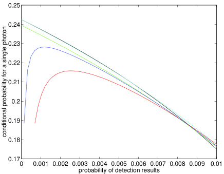
Figure 4: The final probability for a single photon versus the probability for obtaining the appropriate detection results for a four mode interferometer and $p_{\rm max}=0.2$. The black line is the ideal case, the light blue line is that for the case where detection results of $D=3$ and $D=4$ are also allowed, the green line is that if, in addition, the photodetectors have 90% efficiency. The dark blue line is that including all of these experimental limitations, plus 0.1% chance of dark counts at detector 2, and the red line is that taking into account these experimental limitations, as well as allowing 0.1% probability for two photons in the inputs (without dark counts).

To estimate the relative importance of each of the above problems, we have calculated the final conditional probability for a single photon successively taking each of the above issues into account. In Fig. 4, we have plotted the conditional probability for a single photon versus the probability for obtaining the desired combination of detection results. These curves are parametrised by $\epsilon$; that is, both probabilities were calculated for a range of values of $\epsilon$. In general, as $\epsilon$ is decreased, the probability for obtaining the desired detection results decreases, and the final conditional probability for a single photon increases. The particular example we have shown is of a 4 mode interferometer where $p_{\rm max}=0.2$ for the inputs.

To perform these calculations, the density matrix was left unnormalised. The trace of the density matrix at the end of the calculation then gives the probability for that combination of detection results. For those cases where two, three and four photons were not distinguished, the density matrices for these three cases were simply added. To take account of finite efficiency detectors and dark counts, the density matrices for the other detection results were multiplied by constant factors, and added to the density matrix for the desired detection result. It was assumed that the inefficient detectors register single-photon, two-photon and three-photon states as vacuum with probabilities of 10%, 1% and 0.1%, respectively. For the detector on mode 2 it was assumed that a single-photon state is registered as two or more photons with 0.1% probability, and the vacuum state is registered as two or more photons with 0.0001% probability (due to the lower probability of simultaneous dark counts). The appropriate equations to use for the case with multiphoton inputs are derived in Sec. X.

For perfect sources and detectors, the final probability for a single photon is above the initial probability of 20% when the probability for obtaining the detection results is below about 0.7%. Thus, in order to obtain the desired detection results, the experiment needs to be repeated roughly 200 times, which is not unreasonable. If we consider a final detector that can not distinguish between two, three or four photons, the results are almost identical, so this problem is relatively trivial.

Even photodetectors with finite efficiency do not greatly affect the results. If the first two photodetectors have 90% efficiency, the final probability for a single photon is reduced by about 0.3%. The greatest problems are dark counts at detector 2, and multiphoton components at the inputs. If a dark count rate of 0.1% is allowed, then the maximum single-photon probability is reduced below 0.23%. For small values of $\epsilon$ the single-photon probability drops dramatically, rather than approaching the maximum value. The results are similar if a two-photon probability of 0.1% is allowed in the inputs (while the vacuum probability is decreased by 0.1%). The single-photon probability again drops for small values of $\epsilon$, and the maximum single-photon probability is less than 0.22%. For two-photon probabilities of 0.4% or more it is not possible to obtain any increase in the single-photon probability . Thus we see that the main problems with experimental realisations will be two-photon components in the input and dark counts at detector 2.

VIII No-go theorems

In this section, we prove a number of no-go theorems for post-processing via linear optics and photodetection. Note that one limitation of the scheme given in Sec. VI is that it only gives improvements in $R$ for four or modes. In fact, it is impossible to obtain improvements for fewer than four modes BSSK . This result may be shown in the following way. First consider the case $D=0$. Then there is only one term in the sum for $c_{0}$, and $c_{0}=K^{\prime}P_{\bm{0}}$. The expression for $c_{1}$ becomes

$$c_{1} =K^{\prime}\sum_{k=1}^{N}\frac{p_{k}}{1-p_{k}}P_{\bm{0}}\left|\Lambda_{1k}\right|^{2}$$

$$\leq K^{\prime}R_{\rm in}\sum_{k=1}^{N}P_{\bm{0}}\left|\Lambda_{1k}\right|^{2}$$

$$=K^{\prime}R_{\rm in}P_{\bm{0}}$$

$$=c_{0}R_{\rm in}.$$ (44)

Thus we have shown that $R_{\rm out}\leq R_{\rm in}$, so $c_{1}\leq p_{\rm max}$. Hence there can be no improvement in the photon statistics if zero photons are detected.

Figure 5: A U($N$) interferometer can be represented by a U($N-1$) interferometer preceded by $N-1$ beam splitters. This figure shows the example for $N=5$.

This result can also be shown in a more intuitive way as follows. First note that an arbitrary U($N$) interferometer can be obtained using a line of $N-1$ beam splitters followed by a U($N-1$) interferometer (Fig. 5). This is an immediate consequence of the algorithmic construction of arbitrary U($N$) interferometers from beam splitters Reck94 . If the $N-1$ modes upon which the U($N-1$) interferometer acts are those that are measured, then we may omit the U($N-1$) interferometer entirely (because detecting zero photons at the output of this interferometer is identical to detecting zero photons at the input). Thus this case may be reduced to the case of a line of beam splitters where zero photons are detected at each stage.

The case of a line of beam splitters with vacuum detection may be deduced from the case for a single beam splitter. As was shown above, with a single beam splitter there is no improvement in the ratio between the probabilities for detecting one and zero photons. It is easily seen that the same result holds if there are nonzero probabilities for photon numbers larger than 1 in the inputs (corresponding to photon numbers larger than one in the output).

Thus, if we have a line of beam splitters, the ratio between the probabilities for one and zero photons in the output can not be increased above the maximum of that for the inputs. This result implies that the probability of one photon in the output can never exceed $p_{\rm max}$. This result holds for a line of beam splitters, and therefore for an arbitrary U($N$) interferometer.

We can also obtain a similar result for the case $D=1$, provided all the input $p_{i}$ are equal. If the single photon is detected in mode $m$, then

$$c_{0}=K^{\prime}\sum_{k}\frac{p_{\rm max}}{1-p_{\rm max}}P_{\bm{0}}\left|\Lambda_{mk}\right|^{2}=K^{\prime}R_{\rm in}P_{\bm{0}}.$$ (45)

The value of $c_{1}$ is given by

$$c_{1} =\frac{1}{2}K^{\prime}\sum_{k}\sum_{l;l\neq k}R_{\rm in}^{2}P_{\bm{0}}\left|\Lambda_{1l}\Lambda_{mk}+\Lambda_{1k}\Lambda_{ml}\right|^{2}$$

$$\leq\frac{1}{2}K^{\prime}R_{\rm in}^{2}P_{\bm{0}}\sum_{k,l}\left|\Lambda_{1l}\Lambda_{mk}+\Lambda_{1k}\Lambda_{ml}\right|^{2}$$

$$=\frac{1}{2}K^{\prime}R_{\rm in}^{2}P_{\bm{0}}\sum_{k,l}\left[|\Lambda_{1l}|^{2}|\Lambda_{mk}|^{2}+|\Lambda_{1k}|^{2}|\Lambda_{ml}|^{2}+\Lambda_{1l}\Lambda_{mk}\Lambda_{1k}^{*}\Lambda_{ml}^{*}+\Lambda_{1l}^{*}\Lambda_{mk}^{*}\Lambda_{1k}\Lambda_{ml}\right]$$

$$=\frac{1}{2}K^{\prime}R_{\rm in}^{2}P_{\bm{0}}\left[\sum_{l}|\Lambda_{1l}|^{2}\sum_{k}|\Lambda_{mk}|^{2}+\sum_{k}|\Lambda_{1k}|^{2}\sum_{l}|\Lambda_{ml}|^{2}+\sum_{l}\Lambda_{1l}\Lambda_{ml}^{*}\sum_{k}\Lambda_{mk}\Lambda_{1k}^{*}+\sum_{l}\Lambda_{1l}^{*}\Lambda_{ml}\sum_{k}\Lambda_{mk}^{*}\Lambda_{1k}\right]$$

$$=K^{\prime}R_{\rm in}^{2}P_{\bm{0}}.$$ (46)

In the last line we have used the fact that $\Lambda_{1k}$ and $\Lambda_{mk}$ are orthonormal. Thus we again find $R_{\rm out}\leq R_{\rm in}$, so $c_{1}\leq p_{\rm max}$.

These results can be used for an alternative proof that no improvement is possible for the case of a single beam splitter. We have shown that detecting zero photons does not give an improvement, and if one photon is detected, then we must have $M-D=1$ or 0, so there again can be no improvement.

We can also eliminate the case of a three-mode interferometer, though the reasoning is not as straightforward. First note that an input with probability $p_{i}$ of a photon can be obtained by randomly selecting between a source with efficiency $p_{\rm max}$ and the vacuum. That is, with probability $q=p_{i}/p_{\rm max}$ we use the source with efficiency $p_{\rm max}$, and with probability $1-q$ we use the vacuum state. If we discard the information about which source was used, this is obviously equivalent to a source with efficiency $p_{i}$. Hence the value of $c_{1}$ for the source with efficiency $p_{i}$ is the weighted average of the values of $c_{1}$ for the cases where the efficiency is $p_{\rm max}$ and zero. Thus the maximum $c_{1}$ must be obtained with all of the nonzero $p_{i}$ equal to $p_{\rm max}$.

Therefore, in considering the three-mode interferometer, we can let all the nonzero $p_{i}$ be equal to $p_{\rm max}$. If all the $p_{i}$ are nonzero, then we can use the result showing that there is no improvement with one photon detected and all $p_{i}$ equal. The other alternatives for detection have $D=0$ or $M-D\leq 1$, so there can be no improvements in these cases either. If one or more of the $p_{i}$ are zero, then the only detection alternatives are with $D=0$ or $M-D\leq 1$. Thus we have shown that there can never be an increase in the probability of a single photon if less than four modes are used.

IX Unsolved problems

Although it seems that we were able to answer most of the relevant questions concerning the possibility of improving the efficiency of single-photon sources, there are, in fact, still a number of open questions we would now like to address. The two main unsolved problems for this post-processing are:
1. Is it possible to increase the probability for a single photon, regardless of the value of $p_{\rm max}$?
2. Can the single-photon probability be increased without adding a multiphoton component?

At this time the indications are that the answer to both these questions is no. We have performed numerical searches for interferometers that give improvements for $p\geq 1/2$. These searches have been unsuccessful, indicating that it is not possible to obtain an improvement for $p\geq 1/2$. We have not been able to prove this assertion; however, we can show that there are various implications if there is any value of $p_{\rm max}$ such that it is impossible to obtain an improvement.

First note that it is sufficient to use $p_{i}=p_{\rm max}$ in the input modes. As discussed above, for a given interferometer the maximum improvement will always be obtained with all of the nonzero $p_{i}$ equal to $p_{\rm max}$. It is possible to obtain a vacuum state from inputs with efficiency $p_{\rm max}$, simply by using a beam splitter and conditioning on detection of two photons at one of the outputs. Therefore, if there is an interferometer that achieves a certain result using inputs with $p_{i}=0$ or $p_{\rm max}$, there will always be another (expanded) interferometer that achieves the same result with $p_{i}=p_{\rm max}$.

Using this simplification, the expression for $c_{n_{1}}$ simplifies to $c_{n_{1}}=K^{\prime\prime}d_{n_{1}}R_{\rm in}^{n_{1}}/{n_{1}!}$, where

$$d_{n_{1}}=\sum_{\bm{s};\Sigma_{\bm{s}}=\Sigma_{\bm{n}}}\left|S_{\bm{s},\bm{n}}\right|^{2}.$$ (47)

The values of $d_{n_{1}}$ are independent of $p_{\rm max}$, and depend only on the interferometer and combination of detection results. There is an improvement in the probability of a single photon if

$$d_{1}>d_{0}+\sum_{n_{1}=2}^{N}d_{n_{1}}R_{\rm in}^{n_{1}}/{n_{1}!}\,.$$ (48)

Let $p_{0}$ be a value of $p_{\rm max}$ such that there is an improvement in the probability of a single photon, and let the corresponding value of $R_{\rm in}$ be $R_{0}$. Then there exists an interferometer and combination of detection results such that

$$d_{1}>d_{0}+\sum_{n_{1}=2}^{N}d_{n_{1}}R_{0}^{n_{1}}/{n_{1}!}\,.$$ (49)

Since each of the $d_{n}$ are positive, and the right-hand side is increasing as a function of $R_{\rm in}$, we find that (48) is satisfied for all $0<p_{\rm max}\leq p_{0}$. Thus we find that, for any value of $p_{\rm max}$ such that there is an improvement, there is an improvement for all smaller values of $p_{\rm max}$. In turn this result implies that, if there is no improvement for $p_{\rm max}=p_{0}$, then there can be no improvement for larger values of $p_{\rm max}$.

It is also possible to show that, if it were possible to obtain an improvement with no multiphoton contribution, there would be no value of $p_{\rm max}$ for which we can not obtain an improvement. To show this, note that zero multiphoton contribution implies that $d_{n_{1}}=0$ for $n_{1}\geq 2$. Therefore, if this improvement is possible for $p_{\rm max}=p_{0}$, then Eq. (49) becomes simply

$$d_{1}>d_{0}.$$ (50)

Similarly, the condition to obtain an improvement for any other value of $p_{\rm max}$ is simply $d_{1}>d_{0}$, which is automatically satisfied. In addition, because $d_{n_{1}}=0$ for $n_{1}\geq 2$, $c_{n_{1}}=0$ for $n_{1}\geq 2$, for any $p_{\rm max}$.

Thus, if it is possible to obtain an improvement for some value of $p_{\rm max}$ while maintaining zero multiphoton contribution, then it will be possible to obtain an improvement for all values of $p_{\rm max}$. In addition, the relative improvement in $R$ is independent of $p_{\rm max}$. To see this, note that

$$\frac{R_{\rm out}}{R_{\rm in}}=\frac{c_{1}/c_{0}}{R_{\rm in}}=\frac{d_{1}}{d_{0}}.$$ (51)

A further implication is that it would be possible to obtain an output state that is arbitrarily close to the pure single-photon state. As the output from the interferometer has no multiphoton contribution, outputs from $N$ of these interferometers may be used as the input to another, thus increasing $R$ by a factor of $(d_{1}/d_{0})^{2}$. Further iterations may be used to increase $R$ by a factor of $d_{1}/d_{0}$ to any arbitrary power, thus obtaining a final probability for a single photon that is arbitrarily close to 1.

At this stage there is no known scheme that can give an improvement in the probability for a single photon while maintaining zero multiphoton contribution. As shown above, if this were possible for any value of $p_{\rm max}$, then it would be possible for all values $p_{\rm max}$. As increasing the single-photon probability without maintaining zero multiphoton component is a less difficult problem, if it were possible to obtain an improvement while maintaining zero multiphoton component, for all values $p_{\rm max}$ there would be an enormous range of schemes that give improvements without the constraint on the multiphoton component. Such a wide range of schemes would be relatively easy to find numerically; the fact that numerical searches have failed to find any scheme that gives an improvement in the single-photon probability for $p_{\rm max}\geq 1/2$ therefore implies that it is extremely unlikely that there is any scheme that gives an improvement while maintaining zero multiphoton contribution. Nevertheless, these numerical results are not sufficient to rule out this possibility.

X Multiphoton inputs

The majority of this study is based upon inputs from photon sources that have zero multiphoton contribution. It is also possible to derive results for inputs with nonzero probabilities for two or more photons, but this case is more difficult. The simplest case is for a beam splitter with multiphoton inputs. Let us denote the probability for $m$ photons in input mode $i$ by $p_{im}$. Then the input state may be written as

$$\hat{\rho}_{\text{in}}^{(N)} =\sum_{k,l}p_{1k}p_{2l}|{kl}\rangle\langle{kl}|$$

$$=\sum_{k,l}\frac{p_{1k}p_{2l}}{k!l!}(a_{1}^{\dagger})^{k}(a_{2}^{\dagger})^{l}|{00}\rangle\langle{00}|(a_{1})^{k}(a_{2})^{l}.$$ (52)

The beam splitter transformation (3) gives

$$\hat{\rho}_{\rm trans}^{(N)}=\sum_{k,l}\frac{p_{1k}p_{2l}}{k!l!}(\Lambda_{11}a_{1}^{\dagger}+\Lambda_{21}a_{2}^{\dagger})^{k}(\Lambda_{12}a_{1}^{\dagger}+\Lambda_{22}a_{2}^{\dagger})^{l}|{00}\rangle\langle{00}|(\Lambda_{11}^{*}a_{1}+\Lambda_{21}^{*}a_{2})^{k}(\Lambda_{12}^{*}a_{1}+\Lambda_{22}^{*}a_{2})^{l}.$$ (53)

Expanding in a series and conditioning upon detection of $D$ photons gives

$$\hat{\rho}_{\rm out}^{(N)} =K\sum_{k,l}p_{1k}p_{2l}k!l!D!(k+l-D)!\left|\sum_{m=\max(D-k,0)}^{\min(D,l)}\frac{\Lambda_{11}^{D-m}\Lambda_{12}^{m}\Lambda_{21}^{k-D+m}\Lambda_{22}^{l-m}}{(D-m)!m!(k-D+m)!(l-m)!}\right|^{2}$$

$$=KD!\frac{|\Lambda_{22}|^{2D}}{|\Lambda_{12}|^{2D}}\sum_{k,l}p_{1k}p_{2l}k!l!(k+l-D)!|\Lambda_{12}|^{2k}|\Lambda_{22}|^{2l}\left|\sum_{m=\max(D-k,0)}^{\min(D,l)}\frac{(-1)^{m}|\Lambda_{12}/\Lambda_{22}|^{2m}}{(D-m)!m!(k-D+m)!(l-m)!}\right|^{2},$$ (54)

where $K$ is a normalisation constant. If $K$ is omitted, the trace gives the probability for this detection result. This is the expression used to calculate the numerical results in Sec. VII.

The transformation for a multimode interferometer is also straightforward to determine. For this case the input state may be written as

$$\hat{\rho}_{\text{in}}^{(N)} =\bigotimes_{i=1}^{N}\big{[}\sum_{m}p_{im}|{m}\rangle\langle{m}|\big{]}$$

$$=\sum_{\bm{s}}\frac{P_{\bm{s}}}{\prod_{i}s_{i}!}\left(\prod_{i}(\hat{a}_{i}^{\dagger})^{s_{i}}|{0}\rangle\langle{0}|\prod_{i}(\hat{a}_{i})^{s_{i}}\right),$$ (55)

where $P_{\bm{s}}=\prod_{i}(p_{i,s_{i}})^{s_{i}}$. From this point on we use the abbreviated notation $P^{\prime}_{\bm{s}}=P_{\bm{s}}/\prod_{i}s_{i}!$. Note that $s_{i}$ may take any value $\geq 0$, rather than simply 0 and 1. Now applying the interferometer transformation $\hat{\bm{a}}^{\dagger}\mapsto\bm{\Lambda}^{\rm T}\hat{\bm{a}}^{\dagger}$ gives

$$\hat{\rho}_{\rm trans}^{(N)}=\sum_{\bm{s}}P^{\prime}_{\bm{s}}\left[\prod_{i}\left(\sum_{k}\Lambda_{ki}\hat{a}_{k}^{\dagger}\right)^{s_{i}}|{0}\rangle\langle{0}|\prod_{i}\left(\sum_{k}\Lambda_{ki}^{*}\hat{a}_{k}\right)^{s_{i}}\right].$$ (56)

After detection on modes 2 to $N$, the final state obtained is

$$\hat{\rho}_{\rm out}^{(N)}=\sum_{n_{1}=0}^{N}c_{n_{1}}|{n_{1}}\rangle\langle{n_{1}}|.$$ (57)

with

$$c_{n_{1}}=\frac{K^{\prime}}{n_{1}!}\sum_{\bm{s};\Sigma_{\bm{s}}=\Sigma_{\bm{n}}}P^{\prime}_{\bm{s}}\left|S_{\bm{s},\bm{n}}\right|^{2},$$ (58)

where $S_{\bm{s},\bm{n}}=\text{per}(\bm{\Lambda}[\bm{n},\bm{s}])$ and $K^{\prime}$ is a normalisation constant. This result is very similar to the case for inputs with no multiphoton contribution. The only difference is that values of $s_{i}$ larger than 1 are now permitted, and there is the additional dividing factor of $\prod_{i}s_{i}!$. We do not use this result in this paper, but it is a useful general form.

Only one of the no-go theorems still applies for the case where multiphoton inputs are allowed. For the case of a beam splitter, the multiphoton contributions in the input give multiphoton contributions in the output. Therefore, if zero photons are detected, there can be no improvement in the ratio between the probability for one photon to the probability for zero photons. In the multimode case where zero photons are detected, it is possible to decompose the interferometer as in Fig. 5, then omit the U$(N-1)$ interferometer. At each beam splitter in the chain the ratio between the probabilities for one and zero photons is not increased, so the final ratio can not be above the maximum for the inputs. Nevertheless, the result in this case is not as strong as in the case where the inputs have no multiphoton contribution. Proving that the ratio between the probabilities for one and zero photons has not increased does not prove that the absolute probability for a single photon has not increased. The problem is that it is possible, in principle, for the multiphoton component to be decreased sufficiently that the probability for a single photon is increased.

If the inputs have multiphoton contributions, it is not impossible to obtain a perfect single-photon output state. In particular, consider a state $\rho_{0}=\sum_{i}q_{i}|{i}\rangle\langle{i}|$, such that $q_{D}=0$, $q_{D+1}>0$, and $q_{i}=0$ for $i>D+1$. If this state is combined with the vacuum at a beam splitter, and $D$ photons are detected, then the output state will be a pure single-photon state. This result also demonstrates that there is no initial value for the single-photon probability that can not be improved upon.

The drawback to these results is that states such as $\rho_{0}$ would be very difficult to produce in the laboratory. It is likely that there is some measure of the quality of the state that can not be improved upon using linear optics and photodetection. However, it is difficult to determine what measure this would be. For example, it is clear that $\Pi$ can be improved, because $\rho_{0}$ can be heavily super-Poissonian. The same considerations rule out other simple possibilities such as the entropy. Finding a measure that is non-increasing under linear optics and photodetection is a promising direction for future research.

XI Conclusions

Triggered single-photon sources produce an incoherent mixture of zero and one photons, with much smaller probabilities for two or more photons. Provided the multiphoton contributions in the inputs may be ignored, we have shown that it is possible to significantly increase the probability for a single photon by using post-processing via linear optics and photodetection. This method has the drawback that it produces a significant multiphoton component that is comparable to that for the Poisson distribution.

We have shown that there are severe limitations on what post-processing can be performed. In particular, there is an upper limit on the increase in the probability for a single photon. This upper limit can not be achieved, but the method we have found for increasing the probability for a single photon gives the same scaling with the number of modes. It is likely that this method achieves the maximum increase in the probability for a single photon. This result is indicated numerically, but has not been proven.

In addition, it is impossible to obtain an increase in the probability for a single photon using a single beam splitter. Alternatively, if zero photons, or one less than the maximum input photon number are detected, it is again impossible to obtain an improvement in the probability for a single photon. In the restricted case that all the inputs are identical, it is impossible to obtain an improvement in the probability for a single photon if one photon is detected. These no-go theorems are sufficient to prove that at least a four-mode interferometer is required to obtain an improvement.

Another important no-go theorem is that it is impossible to obtain a perfect single-photon output with imperfect inputs. It must be emphasised that this no-go theorem is only for mixed states with no multiphoton components. If we relax these constraints, by considering pure superposition states of zero and one photon, then it is possible to obtain a pure single-photon output. Alternatively, some multiphoton states can be processed to yield a perfect single-photon output. However, it must be emphasised that it is not likely that pure input states, or the appropriate multiphoton states, can be produced experimentally.

There are also a number of important unsolved problems. It is currently unknown whether there is an upper limit (less than 1) to the initial probability for a single photon such that it is possible to obtain an improvement. It is also unknown if it is possible to obtain an improvement in the probability for a single photon while maintaining zero multiphoton contribution. If such a scheme were possible it would be very significant, because it would be possible to obtain a state arbitrarily close to a single photon state from arbitrarily poor input states.