A Practical Scheme for Error Control using Feedback

Abstract

We describe a scheme for quantum error correction that employs feedback and weak measurement rather than the standard tools of projective measurement and fast controlled unitary gates. The advantage of this scheme over previous protocols (for example Ahn et. al, PRA, 65, 042301 (2001)), is that it requires little side processing while remaining robust to measurement inefficiency, and is therefore considerably more practical. We evaluate the performance of our scheme by simulating the correction of bit-flips. We also consider implementation in a solid-state quantum computation architecture and estimate the maximal error rate which could be corrected with current technology.

I Introduction

In the mere space of a decade, quantum information theory has blossomed into a burgeoning field of of experimental and applied research. The initial push for this rapid development was provided by Peter Shor’s discovery of an algorithm that enables quantum computers to find the period of a periodic function much more efficiently than any (known) classical computer algorithm Shor . However, even after Shor’s discovery there was much doubt about the practicality of quantum computing devices due to their fragile nature. The coherencies between systems carrying the quantum information that are crucial to quantum computing algorithms are extremely vulnerable and easily destroyed by unavoidable interactions with the surrounding environment. Furthermore, aside from this decoherence, another concern was the accumulation of errors introduced by imperfect operations performed on the encoded information.

Both these concerns were largely put to rest by the key development of quantum fault tolerance. The error accumulation was shown to be tolerable as long as the systematic error introduced by each operational element was below a critical threshold valueKnill et al. (1998). This threshold result relies heavily upon the development of quantum error correction codes. These codes, the first of which were discovered by Shor Shor (1995) and Steane Steane (1996), redundantly encode information in a manner that allows one to correct errors while preserving coherencies and thus the encoded information.

The main ingredients in the implementation of these error control codes are projective von Neumann measurements that discretize the errors into a finite set, and fast controlled unitary gates that provide the ability to correct any corrupted data. Of course, instantaneous projective measurements and unitary gates are not perfectly implementable in any system; here we will be concerned with the details of how one would actually implement error correction practically on a system where the physical tools available are necessarily physically limited.

We extend previous work Ahn et al. (2002) and describe an implementation of error control that utilizes stabilizer error-correcting codes and employs weak measurement and Hamiltonian feedback to effectively protect an unknown quantum state. This scheme has similarities to the one described previously in Ahn et al. (2002); however, whereas that protocol uses a full state estimation technique that is computationally intensive, this one uses a simple filtering technique that is easily implementable. This protocol is therefore a reasonable one for many of today’s quantum computing architectures.

This paper is organized as follows. Section II reviews the key ideas we use: weak measurement, feedback, and stabilizer codes. Section III describes our error control scheme and two specific instances of it. Section IV describes the simulations performed to analyze the performance of our scheme, presents the results, and considers the effect of measurement inefficiency. Section V examines an actual quantum computer architecture and how this error control protocol could be implemented on this architecture. Section VI concludes.

II Review of concepts

II.1 Quantum feedback control

In order to describe the behavior of a quantum system with feedback, we must first examine the description of an open quantum system undergoing continuous weak measurement; later we will add feedback conditioned on the measurement results. Continuous measurement is modelled by considering the system of interest $\mathcal{S}$ to be weakly coupled to a reservoir $\mathcal{R}$. In order to utilize the Born-Markov approximation, we assume that the self-correlation time of the reservoir is small compared to the time-scales of the system-reservoir coupling and the system dynamics. This essentially says that $\mathcal{R}$ measures $\mathcal{S}$ continuously but quickly forgets, or dissipates away, the result of the measurement. This allows us to write the unconditional dynamics of $\mathcal{S}$ as the following master equation Wiseman (1994a):

$$\dot{\rho}(t)=-i[H,\rho(t)]+\sum_{\mu=1}^{m}\kappa_{\mu}\mathcal{D}[c_{\mu}]\rho(t).$$ (1)

Here $\rho$ is the reduced density matrix of $\mathcal{S}$, $H$ is the system Hamiltonian, $\{c_{\mu}\}$ are the collection of system-reservoir interactions (in our case, where we are considering these interactions to be weak measurements, these are the Hermitian operators corresponding to the observables), $\kappa_{\mu}$ is a parameterization of the coupling strength of $c_{\mu}$, and $\mathcal{D}$ is the decoherence superoperator given by

$$\mathcal{D}[A]\rho=A\rho A^{\dagger}-\frac{1}{2}(A^{\dagger}A\rho+\rho A^{\dagger}A)$$ (2)

for any operator $A$. Note that we set $\hbar=1$ throughout this paper, except for section V.

This equation describes the unconditional dynamics of $\mathcal{S}$ because we are assuming that the measurement records are ignored. That is, ignoring the measurement records corresponding to the observables $\{c_{\mu}\}$ means that the best description of $\mathcal{S}$ we have is one where we average over all possible measurement records, and hence all possible quantum trajectories that the system could have traversed Wiseman (1994a, b).

If we choose not to ignore the measurement records, we instead get a conditional evolution equation for the system Wiseman (1994a, b):

$$d\rho_{c}(t)=-i[H,\rho_{c}(t)]dt+\sum_{\mu=1}^{m}\kappa_{\mu}\mathcal{D}[c_{\mu}]\rho_{c}(t)dt$$

$$+\sum_{\mu=1}^{m}\sqrt{\kappa_{\mu}}\mathcal{H}[c_{\mu}]\rho_{c}(t)dW_{\mu}(t)$$ (3)

where $\rho_{c}$ is the system density operator conditioned on the measurement records of $\{c_{\mu}\}$, $dW_{\mu}(t)$ are Weiner increments (Gaussian distributed random variables with mean zero and autocorrelation $\langle dW(s)dW(t)\rangle=\delta(s-t)dt$) Gardiner (1985), and $\mathcal{H}$ is the superoperator

$$\mathcal{H}[A]\rho=A\rho+\rho A^{\dagger}-\rho~{}\text{tr}[A\rho+\rho A^{\dagger}]$$ (4)

for any operator $A$. The measurement record from the measurement of $c_{\mu}$ is:

$$dQ_{\mu}(t)=\kappa_{\mu}\langle c_{\mu}+c_{\mu}^{\dagger}\rangle_{c}dt+\sqrt{\kappa_{\mu}}dW_{\mu}(t)$$ (5)

where $\langle a\rangle_{c}=\text{tr}(\rho_{c}a)$. In terms of quantum trajectories, this equation corresponds to a diffusive unravelling of the master equation given in Eq. (1). From here onwards, for simplicity we will specialize to the case of $m=1$ in equations (1) and (II.1) (i.e. only one $c_{\mu}$).

Given this model, we can now consider adding feedback to the system. In general, the feedback will be a function of the entire measurement record history. And if we use Hamiltonian feedback, the conditional stochastic master equation (SME) with feedback becomes

$$d\rho_{c}(t) = -i[H,\rho_{c}(t)]dt$$ (6)

$$+\kappa\mathcal{D}[c]\rho_{c}(t)dt+\sqrt{\kappa}\mathcal{H}[c]\rho_{c}(t)dW(t)$$

$$-iR_{Q}(t)[F,\rho_{c}(t)]dt$$

where $R_{Q}(t)$ is some arbitrary function of the entire measurement history $Q(t)$, and $F$ is the feedback Hamiltonian. Note that all we have done is to add a Hamiltonian evolution term whose strength is conditioned by a function of the measurement record.

As shown in Wiseman (1994a), in the restricted case that $R_{Q}(t)$ is a linear function of the measurement value at time $t$ only (i.e. $R_{Q}(t_{0})=f_{linear}[Q(t_{0})]$), we can simplify equation (6) further, and derive a master equation for the unconditional dynamics of the system. This restricted case is often referred to as Markovian feedback, and is considered in connection with quantum error control in Ahn et al. (2003). However, in general, when the feedback is conditioned by a current that is some arbitrary function of the measurement history, it is not possible to treat the evolution analytically, and numerical simulation is the only recourse for solving (6). An important special case of this general feedback is one in which the function $R_{Q}(t)$ is designed to compute an estimate of the state $\rho_{c}(t)$ and output an appropriate feedback strength Doherty and Jacobs (1999); Doherty et al. (2000). We will refer to this as Bayesian feedback, following reference Wiseman et al. (2002). In Ahn et al. (2002) an almost full state estimation is done en route to error control, and here we will consider a simpler and more practical version of that scheme that performs only a partial state estimation.

II.2 Stabilizer codes

In making continuous weak measurements on our system, we would like to choose the measurements in such a manner that we gather as much information about the errors as possible while disturbing the logical qubits as little as possible. These are exactly the conditions satisfiable by encoding the information using a quantum error correcting code; and the powerful stabilizer formalism Gottesman (1997); Nielsen and Chuang (2000) provides a way to easily characterize many of these codes. We will restrict our attention to these stabilizer codes and in this section provide a brief description of the main result of the formalism and give an example. For more detailed discussions, the reader is referred to Gottesman (1997) and Nielsen and Chuang (2000).

We begin by introducing the Pauli group

$$P_{n}=\{\pm 1,\pm i\}\otimes\{I,X,Y,Z\}^{\otimes n}$$ (7)

where $X,Y$, and $Z$ denote the Pauli operators $\sigma_{x},\sigma_{y}$, and $\sigma_{z}$ respectively. To simplify notation, we will omit the tensor product symbol when notating members of $P_{n}$ (e.g. $ZZI\equiv Z\otimes Z\otimes I$).

Now, if we encode $k$ logical qubits in $n$ physical qubits ($n\geq k$), then we can think of errors on our physical system as the action of some subset $\{E_{j}\}\subset P_{n}$ Nielsen and Chuang (2000). Thus, we would like to choose our encoding in a manner that allows us to detect and correct the action of those group elements in $\{E_{j}\}$. The main result from the theory of stabilizer codes tells us about the possibility of choosing such an encoding. It says that provided the elements of $\{E_{j}\}$ satisfy a certain condition, it is always possible to choose a codespace, C, that can be used to detect and correct these error elements Gottesman (1997). Furthermore, this codespace has some special properties:

1. There exist a set of operators in $P_{n}$, called the stabilizer generators and denoted by $g_{1},g_{2},...,g_{r}$, such that every state in C is an eigenstate with eigenvalue +1 of all the stabilizer generators. That is, $g_{i}|{\psi}\rangle=|{\psi}\rangle$ for all $i$ and for all states $|{\psi}\rangle$ in C. Moreover, these stabilizer generators are all mutually commuting.

2. The stabilizer code error correction procedure involves simultaneously measuring all the stabilizer generators and then inferring what correction to apply from the measurement results. The formalism states that the stabilizer measurement results indicate a unique correction operation.

This result tells us that once we identify a set of one qubit errors in $P_{1}$ that we are concerned about, it is possible to choose a stabilizer codespace that can be used to protect the encoded information against such errors. The error detection-correction procedure involves measuring each of the stabilizer generators and then applying a correction corresponding to the results obtained from the stabilizer measurements.

II.3 Example: Three qubit bit-flip code

A common error encountered in quantum computing implementations is the bit flip. This type of error has the effect of reversing the encoded qubit’s value at random times. That is, $|{\psi}\rangle\rightarrow X|{\psi}\rangle$ with probability $p$, and $|{\psi}\rangle\rightarrow|{\psi}\rangle$ with probability $1-p$ (where again, $X\equiv\sigma_{x}$, and $|{\psi}\rangle$ is a one qubit state).

One encoding that protects against this type of error is

$$|{0}\rangle_{L}\equiv|{000}\rangle_{P}$$

$$|{1}\rangle_{L}\equiv|{111}\rangle_{P}$$ (8)

where the right hand side shows the physical encoding in three qubits of the logical qubit value on the left hand side. That is, C $=\textrm{span}\{|{000}\rangle,|{111}\rangle\}$. The stabilizer generators for this codespace are the operators $ZZI$ and $IZZ$. The code can be used to detect and correct any of the errors $XII,IXI$, and $IIX$. The correction procedure involves measuring the two stabilizer generators and then applying the appropriate correcting unitary according to the rules of table 1, which corrects for the bit-flip errors.

ZZI	IZZ	Error	Correcting unitary
+1	+1	None	None
-1	+1	on qubit 1	XII
+1	-1	on qubit 3	IIX
-1	-1	on qubit 2	IXI

Table 1: The three qubit bit-flip code. Note that each error results in a different sequence of stabilizer generator measurement results.

III The error correction scheme

III.1 The general scheme

Once information is encoded using a quantum error-correcting code, conventional error control proposals use projective measurements to measure the stabilizer generators and fast unitary gates to apply the corrections if necessary. In such schemes the detection-correction operation, which is initiated by the projective measurement, happens at discrete time intervals, and these intervals are chosen so that the average number of errors within an interval is correctable. We will refer to such implementations as discrete error correction schemes because of the discrete nature of the detection-correction operation.

In this section we present a protocol that combines weak measurements of the stabilizer generators with feedback to perform continuous error correction. Because of the encoding, these measurements will be unobtrusive when the system is in the codespace and will give error specific information when it is not. However, the requirement of weak measurements makes the measurement currents described by (5) noisy, and therefore ineffective for feedback conditioning. In order to use the information from these measurements to condition the feedback, we must smooth out some of the noise in the currents. The smoothing can be easily done using a low-pass filter; however, such a filtering process introduces its own complications. Specifically, such filtering makes it impossible to derive a master equation describing the evolution because the noise in the feedback signal at time $t$ is not independent of the system state at time $t$. In essence, our smoothing procedure makes Markovian feedback impossible, and leaves the alternative of Bayesian feedback.

Now, full state estimation is a computationally expensive procedure – it most often involves solving an SME in real-time. In fact, as shown in Ahn et al. (2002), the resources needed to apply a full state estimation feedback procedure to quantum error control scale exponentially with the number of qubits in the stabilizer code. Fortunately, we do not need to do a full state estimation. Instead, the coarse-grained state estimate that the stabilizer measurements provide — whether the state is in the codespace or not, and if not, how to correct back into the codespace — is precisely the information needed for error control. That is, instead of estimating $\rho_{c}(t)$, we simply need to reliably identify the stabilizer generator measurement results (in the presence of noise) in order to place $\rho_{c}(t)$ inside or outside the codespace. Furthermore, as seen in the example of section II.3, this information is contained in the signatures of the stabilizer generator measurements (whether they are plus or minus one), a quantity that is fairly robust under the influence of noise. These observations suggest that weak measurement and feedback can be used to continuously detect and correct errors.

The general form of the error correcting scheme we propose is similar to discrete error control, but with a few modifications to deal with the incomplete information gained from the weak measurements. The scheme can be stated in four steps:

1. Encode information in a stabilizer code suited to the errors of concern.

2. Continuously perform weak measurements of the stabilizer generators, and smooth the measurement currents.

3. Depending on the signatures of the smoothed measurement currents, form conditioning signals for feedback operators on each physical qubit. These conditioning currents will be highly non-linear functions of the measurement currents because the conditional switching based on signatures is a non-linear operation.

4. Apply feedback Hamiltonians to each physical qubit, where the strength of the Hamiltonians is given by the conditioning signals formed in the previous step.

Given $m$ stabilizer generators and $d$ errors possible on our system, the SME describing the evolution of a system under this error control scheme is

$$d\rho_{c}(t) = \sum_{k=1}^{d}\gamma_{k}\mathcal{D}[E_{k}]\rho_{c}(t)dt$$ (9)

$$+ \sum_{l=1}^{m}\kappa\mathcal{D}[M_{l}]\rho_{c}(t)dt+\sqrt{\kappa}\mathcal{H}[M_{l}]\rho_{c}(t)dW_{l}(t)$$

$$+ \sum_{k=1}^{d}-iG_{k}(t)[F_{k},\rho_{c}(t)]dt$$

where $\gamma_{k}$ is the error rate for error $E_{k}$, $\kappa$ is the measurement strength (assumed for simplicity to be the same for all measurements $M_{l}$), $F_{k}$ is the feedback Hamiltonian correcting for error $E_{k}$, and $G_{k}$ is the feedback conditioning signal for $F_{k}$. Each $G_{k}$ is a conditional function of the signatures of all the smoothed stabilizer measurements, $\{M_{l}\}$.

Equation (9) has three parts to it: the first line describes the effects of the error operators, the second line describes the effects of the weak stabilizer generator measurements, and the third line describes the effect of the feedback. [Also note that we have set the system Hamiltonian, $H$ in (6), to zero.]

This general scheme is illustrated by the following examples. The systems described by these examples are also the ones simulated in section IV.

III.2 Example: A toy model

This first example is somewhat artificial, but serves as a good illustration of our protocol. The ‘codespace’ we want to protect is simply the state $|{0}\rangle$, the errors are random applications of $X$, and the protocol gathers information by measuring the stabilizer generator $Z$. Obviously this ‘code’ cannot be used for any information processing, but it is useful for investigating the behaviour of our feedback scheme.

The dynamics of this system before the application of feedback are described by the following SME:

$$d\rho_{c}(t) = \gamma\mathcal{D}[X]\rho_{c}(t)dt+\kappa\mathcal{D}[Z]\rho_{c}(t)dt$$ (10)

$$+\sqrt{\kappa}\mathcal{H}[Z]\rho_{c}(t)dW(t),$$

where $\gamma$ is the error rate and $\kappa$ is the measurement rate. The measurement current has the form

$$dQ(t)=2\kappa\langle Z\rangle_{c}(t)dt+\sqrt{\kappa}dW(t),$$ (11)

Now, the measurement of $Z$ reveals whether the systems is in the ‘codespace’ or not because

$$Z|{0}\rangle=+1|{0}\rangle$$

$$Z|{1}\rangle=-1|{1}\rangle.$$ (12)

However, we do not have direct access to $\langle Z\rangle_{c}$, but rather only to the noisy measurement current (11). Therefore we must smooth out the noise on it to obtain error information, and we will choose the following simple filter to do so:

$$R(t)=\frac{1}{\mathcal{N}}\int_{t-T}^{t}e^{-r(t-t^{\prime})}dQ(t^{\prime})$$ (13)

This integral is a convolution in time between the measurement signal and an exponentially decaying signal. In frequency space, this acts as a low pass filter, and thus the output of this operation is a smoothed version of the measurement current with high frequency oscillations removed . The filter parameters $r$ and $T$ determine the decay rate and length of the filter, respectively, and $\mathcal{N}=\frac{2\kappa}{r}(1-e^{-rT})$ serves to normalize $R(t)$ such that it is centred around $\pm 1$.

We will use the signature of this smoothed measurement signal to infer the state of the system and thus to condition the feedback. Explicitly, the form of the feedback conditioning current is

$$G(t)=\left\{\begin{array}[]{ll}R(t)&\textrm{if $R(t)<0$}\\ 0&\textrm{otherwise}\end{array}\right.$$ (14)

Thus, we describe the behaviour of the system with feedback using

$$d\rho_{c}(t) = \gamma\mathcal{D}[X]\rho_{c}(t)dt+\kappa\mathcal{D}[Z]\rho_{c}(t)dt$$ (15)

$$+\sqrt{\kappa}\mathcal{H}[Z]\rho_{c}(t)dW(t)$$

$$-i\lambda G(t)[X,\rho_{c}(t)]dt$$

where $\lambda$ is the maximum feedback strength.

Clearly this feedback conditioning current is non-Markovian (and non-linear). As mentioned above, this makes the Markovian simplification impossible, and therefore the most direct route to evaluating this error correction protocol is numerical simulation. This is done in section IV.

We note at this point that there are several open parameters in the SME (15). These parameters are the following:

1. $\gamma$ - This is the error rate and is largely out of the experimenter’s control.

2. $r$ - The decay rate of the smoothing filter. Large values of $r$ yield responsive measurement currents, while small values of $r$ introduce more delay but make the processed measurement current smoother. We expect there to be some optimal value of $r$ that achieves a trade-off between responsiveness and smoothing ability.

   $r$ is intimately connected to the other filter parameter appearing in (13): $T$, the size of the filter’s memory, which determines how many measurements from the past the filter uses in its calculations. We will choose $T$ to be large enough so that the decaying exponential filter is not truncated prematurely. A $T$ that is some large enough multiple of the filter’s time constant, $1/r$, would be ideal. Since these parameters are dependent on each other, we will only consider one of them ($r$) to be free.

3. $\lambda$ - The maximum strength of the feedback Hamiltonian. The value of this parameter is determined by the physical apparatus and the method of feedback. We expect the performance of the protocol to improve with $\lambda$, because increasing $\lambda$ increases the range of feedback strengths available.

4. $\kappa$ - A parametrization of the measurement strength used in measuring the stabilizer generators. The larger $\kappa$ is the more information we gain from these measurements, and thus we expect the performance to improve with increasing $\kappa$.

In summary, we have three parameters to control - one filter parameter, one feedback parameter, and one measurement parameter. We expect there to be a region in this parameter space where this error control scheme will perform optimally. We will investigate this issue using simulations.

III.3 Example: Bit flip correction

This example is similar to the toy model above but looks at a more realistic error control situation. We will describe the dynamics of a continuous error correction scheme designed to protect against bit flips using the three qubit bit flip code of section II.3.

The measurement currents and SME of the system before the application of feedback are

$$d\rho_{c}(t) = \gamma(\mathcal{D}[XII]+\mathcal{D}[IXI]+\mathcal{D}[IIX])\rho_{c}(t)dt$$ (16)

$$+\kappa(\mathcal{D}[ZZI]+\mathcal{D}[IZZ])\rho_{c}(t)dt$$

$$+\sqrt{\kappa}(\mathcal{H}[ZZI]dW_{1}(t)$$

$$~{}~{}~{}~{}+\mathcal{H}[IZZ]dW_{2}(t))\rho_{c}(t)$$

$$dQ_{1}(t) = 2\kappa\langle ZZI\rangle_{c}(t)dt+\sqrt{\kappa}dW_{1}(t)$$ (17)

$$dQ_{2}(t) = 2\kappa\langle IZZ\rangle_{c}(t)dt+\sqrt{\kappa}dW_{2}(t),$$ (18)

where $\gamma$ is the error rate for each qubit, and $\kappa$ is the measurement strength. We will assume that the errors on different qubits are independent and occur at the same error rate, and also that the measurement strength is the same for both stabilizer generators. (The assumption of identical rates is made for simplicity and can be removed.)

Now, as detailed in table 1, the measurements of $ZZI$ and $IZZ$ reveal everything about the errors. However, as in the toy model, we must smooth the measurement currents in order to gain reliable error information. Therefore, the steps involved in the error correction scheme are the following:

1. Smooth the measurement currents using the following filter:

   $$R_{i}(t)=\frac{1}{\mathcal{N}}\int_{t-T}^{t}e^{-r(t-t^{\prime})}dQ_{i}(t^{\prime})~{}~{}~{}~{}~{}i=1,2$$ (19)

   The definition of this filter is analogous to (13).

2. Depending on the signatures of $R_{1}(t)$ and $R_{2}(t)$ apply the appropriate feedback Hamiltonian. That is,

   1. If $R_{1}(t)<0$ and $R_{2}(t)>0$, apply $XII$.

   2. If $R_{1}(t)>0$ and $R_{2}(t)<0$, apply $IIX$.

   3. If $R_{1}(t)<0$ and $R_{2}(t)<0$, apply $IXI$.

   4. If $R_{1}(t)>0$ and $R_{2}(t)>0$, do not apply any feedback.

   These conditions translate into the following feedback conditioning currents:

   $$G_{1}(t)=\left\{\begin{array}[]{ll}R_{1}(t)&\textrm{if $R_{1}(t)<0$ and $R_{2}(t)>0$}\\ 0&\textrm{otherwise}\end{array}\right.$$ (22)

   $$G_{3}(t)=\left\{\begin{array}[]{ll}R_{2}(t)&\textrm{if $R_{1}(t)>0$ and $R_{2}(t)<0$}\\ 0&\textrm{otherwise}\end{array}\right.$$ (25)

   $$G_{2}(t)=\left\{\begin{array}[]{ll}R_{1}(t)&\textrm{if $R_{1}(t)<0$ and $R_{2}(t)<0$}\\ 0&\textrm{otherwise}\end{array}\right.$$ (28)

Under this scheme, the SME describing the system dynamics with feedback becomes

$$d\rho_{c}(t) = \gamma(\mathcal{D}[XII]+\mathcal{D}[IXI]+\mathcal{D}[IIX])\rho_{c}(t)dt$$ (29)

$$+\kappa(\mathcal{D}[ZZI]+\mathcal{D}[IZZ])\rho_{c}(t)dt$$

$$+\sqrt{\kappa}(\mathcal{H}[ZZI]dW_{1}(t)+\mathcal{H}[IZZ]dW_{2}(t))\rho_{c}(t)$$

$$-i\lambda(G_{1}(t)[XII,\rho_{c}(t)]+G_{2}(t)[IXI,\rho_{c}(t)]$$

$$~{}~{}~{}+G_{3}(t)[IIX,\rho_{c}(t)])dt$$

where $\lambda$ is the maximum feedback strength, which is assumed for simplicity to be the same for all the feedback Hamiltonians.

Again, the non-Markovian feedback signals make numerical simulation the most direct method of solution of this SME.

Also, it is worth noting that even though we gain error information from the signatures of the stabilizer generators, we do not have to wait until the smoothed measurement signals, for example (19), fall below zero before turning on feedback. The feedback conditioning signals, $G_{i}(t)$, can be made non zero as soon as we recognize that the smoothed measurement signals are changing sign. That is, the feedback mechanism can be turned on as soon as we see a significant shift in the stabilizer generator measurements from their error free value: one. We can state this ‘significant’ shift more precisely as a change of more than $n$ standard deviations from the mean value of one, for $n$ sufficiently large. Thus the choice of $n$ depends on the signal-to-noise ratio of the smoothed measurement currents, and therefore on the parameters $r$ and $\kappa$.

IV Simulation Results

As a way of evaluating the performance of the general error control scheme using weak measurements and feedback, we numerically solved the SMEs described in the two examples of section III. A comparison of the SMEs (15) and (29) shows that the one qubit toy model has all the free parameters of the full three qubit code, and therefore is a good model on which to explore the parameter space formed by $r,\lambda,$ and $\kappa$. This is useful because the smaller state space of the toy model makes simulating it far more computationally tractable than simulating the bit-flip correction example.

IV.1 The toy model

We chose to simulate the dynamics of (15) by way of an associated stochastic Schrödinger equation (SSE) for two reasons: (i) it is less computationally intensive, (ii) it allows us to look at individual trajectories of the system if desired. The form of this associated SSE is as follows:

$$d|{\psi_{c}(t)}\rangle=dN(t)(X|{\psi_{c}(t)}\rangle-|{\psi_{c}(t)}\rangle)~{}+~{}\sqrt{\kappa}~{}dW(t)(Z-\langle Z\rangle(t))~{}|{\psi_{c}(t)}\rangle~{}-~{}\frac{\kappa}{2}(1-\langle Z\rangle(t)Z)^{2}~{}|{\psi_{c}(t)}\rangle dt~{}-~{}i\lambda G(t)X~{}|{\psi_{c}(t)}\rangle dt$$ (30)

where $dN(t)$ is a point process increment (in the number of errors) described by

$$dN(t)^{2} = dN(t)$$ (31)

$$E[dN(t)] = \gamma dt.$$ (32)

That is, $dN$ is a random variable that is either 0 or 1 at each time step, and is distributed according to the error rate $\gamma$. A graph of the process $dN(t)$ would be a sequence of Poisson distributed (with parameter $\gamma$) spikes. In the language of quantum trajectories, this SSE is simply one possible unravelling of the SME (15).

The SSE was solved using Euler numerical integration with time steps $dt=10^{-4}$. When ensemble averages were required — that is, when we were interested in the behaviour of $\rho_{c}(t)$ — 600 trajectories were averaged over. To evaluate the performance of the protocol, we used the codeword fidelity: $F(t)=\langle{\psi(0)}|\rho(t)|{\psi(0)}\rangle$. Here, $|{\psi(0)}\rangle$ is the initial state of the system, which is taken to be $|{0}\rangle$ unless otherwise specified.

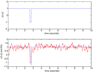
Figure 1: A sample trajectory of the one qubit ”code” with feedback. The top graph just shows the expectation value of $Z$, and the bottom graph shows expectation value of $Z$ and the filtered signal $R(t)$.

Figure 1 shows a sample trajectory from the one qubit simulation. The figure shows the expectation value of the $Z$ measurement as a function of time and also the superimposed filtered measurement signal, $R(t)$. The transitions (of expectation value of $Z$) to $-1$ are due to errors, and the transitions back to $+1$ are due to feedback correction.

We used this toy model primarily to gain insight into the choice of parameters that lead to optimal error correction. The conclusions drawn from exploring the parameter space using this one qubit simulation are the following:

1. The decay rate of the filter, $r$, should be determined by the strength of the feedback, $\lambda$. That is, given a strong feedback Hamiltonian, it is necessary to have a responsive conditioning current; one with little memory.

2. As expected, the larger the measurement strength $\kappa$, the better the protocol performs.

3. Performance also improves as $\lambda$, the feedback strength, is increased. This is to be expected because as $\lambda$ is increased, the range of the strength of the feedback Hamiltonian increases leading to a greater degree of control.

4. The interplay between the two processes – measurement and feedback – must be considered. In particular, larger values of $\kappa$ will yield better performance only if these values are not too much larger than the value of $\lambda$. That is, if the measurement strength is much stronger than the feedback strength, the measurement process disrupts the feedback correction process and makes it ineffective. Therefore the magnitude of the measurement strength should be less than, or of the same order of magnitude, as the feedback Hamiltonian strength.

Given the strong dependence between parameters that these one qubit simulations identify, there are really only three free parameters in the system: $\kappa,\lambda$ and $\gamma$. Since the last is out of the experimenter’s control, there remain two controllable parameters. In practice, neither of these parameters, the measurement strength or the feedback strength, are completely configurable. The physical implementation scheme typically limits the range of these parameters, and in section V we shall see whether the practical ranges for one particular implementation allows for error control via this feedback scheme.

It is instructive to note that the free parameters of the protocol are all physical parameters. That is, the optimal operating regime of the protocol is defined by the system’s physical features rather than the introduced filter. Therefore, it is possible to design a filter that allows the protocol to perform optimally for a given set of physical parameters ($\kappa$ and $\lambda$).

IV.2 Three qubit code simulation

Now we move on to the simulation of the three qubit bit flip code. This simulation behaves in much the same way as the one qubit version, but with one key difference: for the one qubit ‘code’, a double error event – where an error occurs on the qubit before we have corrected the last error – is not too damaging: in this case, the error correcting feedback mechanism detects a traversal back into the ‘codespace’ and thus stops correcting. In the three qubit code, this situation is a little more complicated. Let us consider the situation in which a second error happens while a previous error is being corrected. If this second error happens to be on the same qubit as the one being corrected, then in consonance with the one qubit ‘code’, it is not too damaging. However, if the second error is on one of the two qubits not being corrected, an irrecoverably damaging event occurs, because in this case the stabilizer measurements cease to provide accurate information about the error location, and the protocol’s ‘corrections’ actually introduce errors.

This identifies a key consideration in any continuous, feedback based error correction scheme. The finite duration of the detection and correction window means that we must choose our parameters with this finite window small enough that the probability of an error we cannot correct (in this case, two errors on different qubits) is negligible. This is analogous to choosing the detection-correction intervals in the discrete error control case to be small enough to avoid uncorrectable errors.

The SSE that describes the dynamics of the three qubit error correction scheme is

$$d|{\psi_{c}(t)}\rangle = dN_{1}(t)(XII|{\psi_{c}(t)}\rangle-|{\psi_{c}(t)}\rangle)~{}+~{}dN_{2}(t)(IXI|{\psi_{c}(t)}\rangle-|{\psi_{c}(t)}\rangle)~{}+~{}dN_{3}(t)(IIX|{\psi_{c}(t)}\rangle-|{\psi_{c}(t)}\rangle)$$ (33)

$$+ \sqrt{\kappa}~{}dW_{1}(t)(ZZI-\langle ZZI\rangle(t))~{}|{\psi_{c}(t)}\rangle~{}+~{}\sqrt{\kappa}~{}dW_{2}(t)(IZZ-\langle IZZ\rangle(t))~{}|{\psi_{c}(t)}\rangle$$

$$- \frac{\kappa}{2}(1-\langle ZZI\rangle(t)ZZI)^{2}~{}|{\psi_{c}(t)}\rangle dt~{}-~{}\frac{\kappa}{2}(1-\langle IZZ\rangle(t)IZZ)^{2}~{}|{\psi_{c}(t)}\rangle dt$$

$$- i\lambda G_{1}(t)XII~{}|{\psi_{c}(t)}\rangle dt~{}-~{}i\lambda G_{2}(t)IXI~{}|{\psi_{c}(t)}\rangle dt~{}-~{}i\lambda G_{3}(t)IIX~{}|{\psi_{c}(t)}\rangle dt.$$

This SSE is of course an unravelling of SME (29), and all parameters are defined as for that equation.

As in the one qubit case, we solved this differential equation using an Euler method with timesteps $dt=10^{-4}$. Again, ensemble averages were done over 600 trajectories when needed. The initial state used was $|{000}\rangle$, and the performance was measured using the codeword fidelity $F_{3}(t)=\langle{000}|\rho(t)|{000}\rangle$. A true fidelity measure of the protocol performance would average over all possible input states; however, because $|{000}\rangle$ is most susceptible to bit flip errors, the fidelity we use can be considered a worst case performance analysis.

The performance of the error correction scheme using this code is summarized by figure 2. This figure shows the fidelity versus time curves ($F_{3}(t)$) for several values of error rate ($\gamma$). Each plot also shows the fidelity curve ($F_{1}(t)$) for one qubit in the absence of error correction. A comparison of these two curves shows that the fidelity is preserved for a longer period of time by the error correction scheme for small enough error rates. Furthermore, for small error rates ($\gamma<0.3$) the $F_{3}(t)$ curve shows a vast imrpovement over the exponential decay in the absence of error correction. However, we see that past a certain threshold error rate, the fidelity decay even in the presence of error correction behaves exponentially, and the two curves look very similar; past the threshold, the error correcting scheme becomes unable to handle the errors and becomes ineffective. In fact, although not completely evident from the figure, well above the threshold the performance of the scheme becomes worse than the unprotected qubit’s performance. This poor performance results from the feedback ‘corrections’ being so inaccurate that the feedback mechanism effectively increases the error rate.

The third line in the plots of figure 2 is of the average fidelity achievable by discrete quantum error correction –using the same three qubit code– when the time between the detection-correction operations is t. The value of this fidelity ($F_{3d}(t)$) as a function of time was analytically calculated in Ahn et al. (2002),

$$F_{3d}=\frac{1}{4}(2+3e^{-2\gamma t}-e^{-6\gamma t}).$$ (34)

A comparison between $F_{3}(t)$ and $F_{3d}(t)$ highlights the relative merits of the two schemes. The fact that the two curves cross each other for large $t$ indicates that if the time between applications of discrete error correction is sufficiently large, then a continuous protocol will preserve fidelity better than a corresponding discrete scheme. In fact, this comparison suggests that a hybrid scheme, where discrete error correction is performed relatively infrequently on a system continuously protected by a feedback protocol, might be a viable approach to error control.

All the $F_{3}(t)$ curves show an exponential decay at very early times, $t\approx 0$ to $t\approx 0.1$. This is an artifact of the finite filter length and our specific implementation of the protocol. In particular, our simulation does not smooth the measurement signal until enough time has passed to get a full buffer of measurements; that is, filtering and feedback only start at $t=T$. Of course, this can be remedied by a more complicated scheme that smoothes the measurement signal and applies feedback even when it has access to fewer than $T/dt$ measurements.

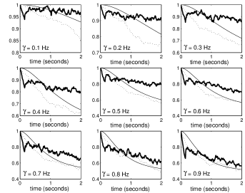
Figure 2: Fidelity curves with and without error correction for several error rates. The thick solid curve is the fidelity of the three qubit code with error correction, $F_{3}(t)$ (parameters used: $dt=10^{-4}s,\kappa=150~{}Hz,\lambda=150~{}Hz,r=20~{}Hz,T=1500\times dt~{}s$). The dotted curve is the fidelity of one qubit without error correction, $F_{1}(t)$. And the thin solid curve is the fidelity achievable by discrete quantum error correction when the duration between applications is t, $F_{3d}(t)$.

IV.3 Inefficient measurement

We have modeled all our measurement processes as being perfect. In reality, detectors will be inefficient and thus yield imperfect measurement results. This ineffiency is typically represented by a parameter $\eta$ that can range from 0 to 1, where 1 denotes a perfect detector. How is this feedback protocol affected by non-unit efficiency detection?

To examine this question, we simulated the three qubit code with inefficient detection. The evolution SME and the measurement currents in the presence of inefficient detection are as follows:

$$d\rho_{c}(t) = \gamma(\mathcal{D}[XII]+\mathcal{D}[IXI]+\mathcal{D}[IIX])\rho_{c}(t)dt$$ (35)

$$+\kappa(\mathcal{D}[ZZI]+\mathcal{D}[IZZ])\rho_{c}(t)dt$$

$$+\sqrt{\kappa\eta}(\mathcal{H}[ZZI]dW_{1}(t)+\mathcal{H}[IZZ]dW_{2}(t))\rho_{c}(t)$$

$$-i\lambda(G_{1}(t)[XII,\rho_{c}(t)]+G_{2}(t)[IXI,\rho_{c}(t)]$$

$$~{}~{}~{}+G_{3}(t)[IIX,\rho_{c}(t)])dt$$

$$dQ_{1}(t) = 2\kappa\sqrt{\eta}\langle ZZI\rangle_{c}(t)dt+\sqrt{\kappa}dW_{1}(t)$$ (36)

$$dQ_{2}(t) = 2\kappa\sqrt{\eta}\langle IZZ\rangle_{c}(t)dt+\sqrt{\kappa}dW_{2}(t)$$ (37)

where $0<\eta\leq 1$ is the measurement efficiency, and all other quantities are the same as in equations (16) and (29).

The results of these simulations are summarized by figure 3. The decay of fidelity with decreasing $\eta$ indicates that inefficient measurements have a negative effect on the performance of the protocol as expected. However, the slope of the decay is very small— in particular, the graph does not exponentially decay as do Markovian feedback protocols— and this suggests that this protocol has a certain tolerance to inefficiencies in measurement. This is reasonable because the filtering process in the protocol has the effect of improving the quality of the measurements and thus negating some of the ill effects of the inefficient measurements. Also, as in the full state estimation protocol of Ahn et al. (2002), because the feedback conditioning current is a function of a measurement record history —as opposed to just the current measurement— errors induced by inefficient measurement tend not to be so damaging. Here we see the true strength of this error correction scheme: it combines the robustness of a state estimation based feedback protocol with the practicality of a Markovian feedback protocol.

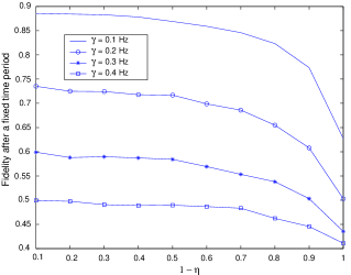
Figure 3: Average fidelity after a fixed amount of time as a function of 1-efficiency for several error rates (parameters used: $dt=10^{-4}s,\kappa=50~{}Hz,\lambda=50~{}Hz,r=10~{}Hz,T=1500\times dt~{}s$).

V Links to experiment

In this section we study the possibility of applying this error correction technique to a particular quantum computing architecture.

V.1 Solid-state quantum computing with RF-SET readout

Several schemes for solid-state quantum computing have been proposed Kane (1998); Loss and DiVincenzo (1998); Tanamoto (2000); Nakumura et al. (1999). These use the charge or spin degree of freedom of single particles to represent logical qubits, and measurement involves probing this degree of freedom.

Here we examine the weak measurement of one such proposal that uses coherently coupled quantum dots (CQDs) and an electron that tunnels between the dotsHollenberg et al. (2003). The dots are formed by two P donors in Si, separated by a distance of about 50nm. Surface gates are used to remove one electron from the double donor system leaving a single electron on the P-P⁺ system. This system can be regarded as a double well potential. Surface gates can then be used to control the barrier between the wells as well as the relative depth of the two wells. Using surface gates, the wells can be biased so that the electron can be well localised on either the left $|L\rangle$ or the right $|R\rangle$ of the barrier. These (almost) orthogonal localised states are taken as the logical basis for the qubit, $|{0}\rangle=|{L}\rangle,\ \ |{1}\rangle=|{R}\rangle$. It is possible to design the double well system so that, when the well depths are equal, there are only two energy eigenstates below the barrier. These states are the symmetric ground state $|{+}\rangle$ and the antisymmetric first excited state $|{-}\rangle$. A state localised on the left (right) of the barrier is then well approximated as a linear superposition of these two states,

$$|L\rangle = \frac{1}{\sqrt{2}}(|+\rangle+|-\rangle)$$ (38)

$$|R\rangle = \frac{1}{\sqrt{2}}(|+\rangle-|-\rangle)$$ (39)

An initial state localised in one well will then tunnel to the other well at the frequency $\Delta=(\epsilon_{+}-\epsilon_{-})/\hbar$ where $\epsilon_{\pm}$ are the two energy eigenstates below the barrier.

The Pauli matrix, $Z=|L\rangle\langle L|-|R\rangle\langle R|$, is diagonal in this localised state basis. The Hamiltonian for the system can be well approximated by

$$H=\hbar\frac{\omega(t)}{2}Z+\hbar\frac{\Delta(t)}{2}X$$ (40)

where $X=|L\rangle\langle R|+|R\rangle\langle L|$. Surface gates control the relative well depth $\hbar\omega(t)$ (a bias gate control) and the tunnelling rate $\Delta(t)$, (a barrier gate control) which are therefore time dependent. For non-zero bias the energy gap between the ground state and the first excited state is $E(t)=\hbar\sqrt{\omega(t)^{2}+\Delta(t)^{2}}$. Further details on the validity of this Hamiltonian and how well it can be realised in the PP⁺ in Si system can be found in Barrett and Milburn (2003).

A number of authors have discussed the sources of decoherence in a charge qubit system such as this oneBarrett and Milburn (2003); Fedichkin and Fedorov (2003); Hollenberg et al. (2003). For appropriate donor separation, phonons can be neglected as a source of decoherence. The dominant sources of decoherence then arise from fluctuations in voltages on the surface gates controlling the Hamiltonian and electrons moving in and out of trap states in the vicinity of the dot. This latter source of decoherence is expected to occur on a longer time scale and is largely responsible for $1/f$ noise in these systems. In any case both sources of decoherence can be modelled using the well known spin-boson model Weiss (1999). The key element of this model for the discussion here is that the interaction energy between the qubit and the reservoir is a function of $Z$.

If the tunnelling term proportional to $\Delta(t)X$ in Eq. (40) were not present, decoherence of this kind would lead to pure dephasing. However, in a general single qubit gate operation, both dephasing and bit flip errors can arise in the spin-boson model. We can thus use the decoherence rate calculated for this model as the bit flip error rate in our feedback error correction model. We will use the result from the detailed model of Hollenberg et al. Hollenberg et al. (2003) for a device operating at 10K, and set the error rate $\gamma=1.4\times 10^{6}\mbox{s}^{-1}$. This rate could be made a factor of ten smaller by operating at lower temperatures and improving the electronics controlling the gates.

We now turn to estimating the measurement rate , $\kappa$, for the PP⁺ system. In order to readout the qubit in the logical basis we need to distinguish a single electron in the left or the right well quickly and with high probability of success (efficiency). The technique of choice is currently based on radio frequency single electron transistors (RF-SET)Schoelkopf et al. (1998). We will use the twin SET implementation of Buehler et al. Buehler et al. (2003).

In an RF SET the Ohmic load in a tuned tank circuit comprises a single electron transistor with the qubit acting as a gate bias. The two different charge states of the qubit provide two different bias conditions for the SET, producing two different resistive loads, and thus two levels of power transmitted through the tank circuit. The electronic signal carries a number of noise components: for example, the Johnson-Nyquist noise of the circuit, random changes in the SET bias conditions due to fluctuating trap states in the SET, etc. The measurement must be operated in such a way that the charge state of the qubit can be quickly discerned as a departure of the signal from some fiducial setting, despite the noise. Clearly it takes some minimum time interval, $t_{M}$, to discriminate a qubit signal change from a random noisy fluctuation. We need to keep the measurement time as short as possible. However if the measurement time is too short, one may mistake a large fluctuation, due to a non-qubit based change in bias conditions, for the real signal. In other words one may mistake a 1 for a 0, and vice versa. The probability of this happening is the efficiency of the measurement, $\eta(t_{M})$, which depends on the measurement time. The key performance parameters are (i) the measurement time, $t_{M}$, and (ii) the efficiency $\eta(t_{M})$. An additional parameter that is often quoted is the minimum charge sensitivity per root hertz, $S$. Given $t_{M}$, $S$ determines a minimum change in the charge, $\Delta q$, that can be seen by the RF-SET at a given bias condition. In Buehler et al. (2003), a measurement time of $t_{M}=6\times 10^{-6}\mbox{s}$ was found for a signal of $\Delta q=0.2e$ and an efficiency of $10^{-6}$. We now need to relate this measurement time to the measurement decoherence rate parameter, $\kappa$, of our ideal feedback model.

If the measurement were truly quantum limited (that is to say, the signal-to-noise ratio is determined only by the decoherence rate $\kappa$), the inverse measurement time would be of the same order of magnitude as the decoherence rate (see Goan (2003)). The measurement described in Buehler et al.Buehler et al. (2003) will almost certainly not be quantum limited. However, here we will assume the measurement to be quantum limited, so as to obtain a lower limit to the measurement decoherence rate. Thus we take $\kappa=10^{6}\mbox{s}^{-1}$.

We next need to estimate typical values for the feedback strength. From Eq. (15) we see that the feedback Hamiltonian is proportional to an $X$ operator. In the charge qubit example, this corresponds to changing the tunneling rate for each of the double dot systems that comprise each qubit. The biggest tunneling rate ($\Delta$) occurs when the bias of the double wells makes it symmetric. In Barrett and Milburn (2003), the maximum tunneling rate is about $10^{9}$ s^-1, for a donor separation of 40nm. A large tunneling rate makes for a fast gate, and thus a fast correction operation. Thus the maximum value of $\lambda$ can be taken to be $10^{9}$ s^-1.

To summarise, in the PP⁺ based charge qubit, with RF-SET readout, we have $\gamma\approx\kappa\approx 10^{6}\mbox{s}^{-1}$, and $\lambda\approx 10^{9}\mbox{s}^{-1}$.

The fact that the measurement strength and the error rate are of the same order of magnitude for this architecture is a problem for our error correction scheme. This means that the rate at which we gain information is about the same as the rate at which errors happen, and it is difficult to operate a feedback correction protocol in such a regime. Although it is unlikely that the measurement rate could be made significantly larger in the near future, as mentioned above it is possible that the error rate could be made smaller by improvements in the controlling electronics. Thus it is interesting to consider how low the error rate would have to be pushed before our error control scheme becomes effective. To answer this question we ran the three qubit bit flip code simulation using the parameters stated above and lowered the error rate until the error control performance was acceptable. We found that the fidelity after 1ms could be kept above 0.8 on average if the error rate, $\gamma$, is below $10^{2}$ s^-1 (with $\kappa=10^{6}$ s^-1, and $\lambda=10^{7}$ s^-1). So we see that a difference in order of magnitude of four between the measurement and feedback strengths, and the error rate, is about what this protocol (using the three qubit code) requires for reasonable performance. That is, we require

$$\frac{\kappa}{\gamma}\approx\frac{\lambda}{\gamma}\approx 10^{4}$$ (41)

Of course, depending on the performance requirements this ratio may be larger or smaller. Also, a full optimization of the filter used in the scheme is likely to drive this ratio down by up to an order of magnitude.

We can compare the requirements of the three-qubit code with the one-qubit version. Given the same measurement and feedback parameters ($\kappa=10^{6}$ s^-1, $\lambda=10^{7}$ s^-1), the one-qubit ‘code’ can keep the fidelity above 0.8 after 1ms when $\kappa/\gamma\approx\lambda/\gamma\approx 10$. That is, only one order of magnitude difference is required between the error rate and the measurement and feedback rates. This suggests that a key issue with feedback based error correction schemes is scalability. The ratio between measurement and feedback rates and error rate has to increase along with the error correcting code size (in qubits).

VI Discussion and Conclusion

We have described a practical scheme for implementing error correction using continuous measurement and Hamiltonian feedback. We have demonstrated the validity of the scheme by simulating it for a simple error correction scenario.

As the simulations show, this error control scheme can be made very effective if the operational parameters (measurement strength, feedback strength, filter parameters) are well matched to the error rate of a given sytem. At the same time, the scheme uses relatively modest resources and thus is easy to implement, as well as being robust in the face of measurement inefficiencies.

From a quantum control perspective, an interesting feature of this protocol is the encoding. That is, despite using state estimate feedback, the protocol requires little side processing due to the fact that instead of a full state estimate, it uses a coarse-grained state estimate naturally suggested by the encoding. In control theory terms, this simplification is a result of the specific choice of control state space (what to observe and control); a choice dictated by the stabilizer encoding and measurements. It would be interesting to examine the general conditions under which an encoding is available that allows for practical, efficient state estimate feedback control.

The possibility of using continuous error correction in combination with its discrete counterpart is an interesting possibility. Such a scheme has the potential to significantly improve the stability of quantum memories, and the implications of such a combination scheme for fault tolerance would be worth investigating.

We also studied a solid-state quantum computing architecture with RF-SET readout and the feasibility of implementing this error correction protocol on it. Although the measurement and feedback rates currently possible on this architecture do not allow for error correction via this feedback scheme with the intrinsic error rate, it is foreseeable that as the controlling technology improves, this error control scheme will become possible on this architecture. From numerical simulations, we found the approximate parameter regime where the three qubit code using this scheme becomes effective – that is, exactly how much improvement is necessary before the scheme becomes feasible. It would be interesting to investigate this further and explore more rigorously how values of $\kappa/\gamma$ and $\lambda/\gamma$ dictate protocol performance as well as the exact dependency of these parameter ratios on the code size. Such an investigation will be crucial in addressing the issue of scalability of this error control scheme.

VII Acknowledgements

We gratefully acknowledge the support of the Australian Research Council Centre of Excellence in Quantum Computer Technology. Part of this research was done using the resources of the Visualisation and Advanced Computing Laboratory at the University of Queensland. MS would like to thank Mr. James Lever for his assistance and support at this facility. CA is grateful for the hospitality of the Centre for Quantum Computer Technology at the University of Queensland and acknowledges support from an Institute for Quantum Information fellowship.

References

- (1) P. W. Shor, Polynomial-time algorithms for prime factorization and discrete logarithms on a quantum computer, (NOTE: This is a revised version of the original paper), eprint quant-ph/9508027.
- Knill et al. (1998) E. Knill, R. Laflamme, and W. H. Zurek, Proc. R. Soc. London A 454, 365 (1998).
- Shor (1995) P. Shor, Phys. Rev. A 52, 2493 (1995).
- Steane (1996) A. M. Steane, Phys. Rev. Lett. 77, 793 (1996).
- Ahn et al. (2002) C. Ahn, A. D. Doherty, and A. J. Landahl, Phys. Rev. A 65, 042301 (2002).
- Wiseman (1994a) H. M. Wiseman, Ph.D. thesis, The University of Queensland (1994a).
- Wiseman (1994b) H. M. Wiseman, Phys. Rev. A 49, 2133 (1994b).
- Gardiner (1985) C. W. Gardiner, Handbook of Stochastic Methods (Springer, 1985).
- Ahn et al. (2003) C. Ahn, H. M. Wiseman, and G. J. Milburn, Phys. Rev. A 67, 052310 (2003).
- Doherty and Jacobs (1999) A. Doherty and K. Jacobs, Phys. Rev. A 60, 2700 (1999).
- Doherty et al. (2000) A. C. Doherty, S. Habib, K. Jacobs, H. Mabuchi, and S. M. Tan, Phys. Rev. A 62, 012105 (2000).
- Wiseman et al. (2002) H. M. Wiseman, S. Mancini, and J. Wang, Phys. Rev. A 66, 013807 (2002).
- Gottesman (1997) D. Gottesman, Ph.D. thesis, Caltech (1997).
- Nielsen and Chuang (2000) M. A. Nielsen and I. L. Chuang, Quantum Computation and Quantum Information (Cambridge University Press, 2000).
- Oppenheim et al. (1996) A. V. Oppenheim, A. S. Willsky, and S. Hamid Nawab, Signal and Systems (Prentice Hall, 1996), 2nd ed.
- Kane (1998) B. E. Kane, Nature (London) 393, 133 (1998).
- Loss and DiVincenzo (1998) D. Loss and D. P. DiVincenzo, Phys. Rev. A 57, 120 (1998).
- Tanamoto (2000) T. Tanamoto, Phys. Rev. A 61, 22305 (2000).
- Nakumura et al. (1999) Y. Nakumura, Y. A. Pashkin, and J. S. Tsai, Nature 398, 786 (1999).
- Hollenberg et al. (2003) L. C. L. Hollenberg, A. S. Dzurak, C. Wellard, A. R. Hamilton, D. J. Reilly, G. J. Milburn, and R. G. Clark, Phys. Rev. B (Brief Reports). In Press. (2003).
- Barrett and Milburn (2003) S. D. Barrett and G. J. Milburn, Phys. Rev. B 68, 155307 (2003).
- Fedichkin and Fedorov (2003) L. Fedichkin and A. Fedorov (2003), eprint quant-ph/0309024.
- Weiss (1999) U. Weiss, Quantum Dissipative Systems (World Scientific, 1999).
- Schoelkopf et al. (1998) R. J. Schoelkopf, P. Wahlgren, A. A. Kozhevnikov, P. Delsing, and D. E. Prober, Science 280, 1238 (1998).
- Buehler et al. (2003) T. M. Buehler, D. J. Reilly, R. P. Starrett, A. Greentree, A. R. Hamilton, A. S. Dzurak, and R. G. Clark, Phys. Rev. B (Rapid). Submitted. (2003).
- Goan (2003) H. S. Goan, Quant. Inf. and Comp. 3, 121 (2003).