Bloch Equations and Completely Positive Maps

Abstract

The phenomenological dissipation of the Bloch equations is reexamined in the context of completely positive maps. Such maps occur if the dissipation arises from a reduction of a unitary evolution of a system coupled to a reservoir. In such a case the reduced dynamics for the system alone will always yield completely positive maps of the density operator. We show that, for Markovian Bloch maps, the requirement of complete positivity imposes some Bloch inequalities on the phenomenological damping constants. For non-Markovian Bloch maps some kind of Bloch inequalities involving eigenvalues of the damping basis can be established as well. As an illustration of these general properties we use the depolarizing channel with white and colored stochastic noise.

I Introduction

In 1946, Felix Bloch introduced a set of equations describing the dynamics of a nuclear induction of a spin that interacts with a magnetic field Bloch (1946). The applied magnetic field drives the Bloch vector of the magnetic moment, causing it to precess about the field direction. In addition to the unitary evolution describing the magnetic moment precession, a nonunitary evolution is observed in nuclear magnetic resonance, which results in dissipation of the magnetic observables. This dissipation is characterized by two phenomenological decay constants. The two lifetimes $T_{1}$ and $T_{2}$ are the longitudinal and transverse decay constants, respectively.

Fluctuations in the environment, such as inhomogeneities in the magnetic field and interactions with other moments, lead to dissipation in the system. The dissipation constants $T_{1}$ and $T_{2}$ are nonnegative so that exponential decay of the magnetic moment occurs. It is well known that this condition is required to preserve the positivity of the density operator under dissipation. The phenomenological dissipation of the Bloch vector defines a positive map (PM) of the density operator for the spin system.

About the physical sources of the dissipation constants Bloch wrote:

The actual value of $T_{1}$ is very difficult to predict for a given substance … To give a reliable estimate of $T_{2}$ … requires a more detailed investigation of the mechanism involved and will not be attempted here.

In the same paper Bloch made the following statement about the relative values of the dissipation constants:

… serious errors may be committed by assuming $T_{1}=T_{2}$ . There are, on the other hand, also cases where this equality is justified …

It took almost 30 years to understand that the dissipation results from a reduction of a unitary evolution of a system coupled to a quantum reservoir. In the process of such a reduction, the transformation of the density operator of the system has to be a completely positive map (CPM). However, if the hypothesis of complete positivity is to be imposed then the values of the dissipation constants cannot be arbitrary. In particular, the inequality $2T_{1}\geq T_{2}$ must hold and has been experimentally observed Abragan (19610).

It is the purpose of this paper to reexamine the well-known Bloch equations in the context of completely positive maps. We show that the condition of complete positivity for Markovian Bloch maps imposes some Bloch inequalities on the phenomenological damping constants. For non-Markovian Bloch maps, generalized Bloch inequalities involving eigenvalues of the damping basis can be established as well. The depolarizing channel with white noise is used to illustrate these general properties. The non-Markovian Bloch map is studied in the framework of a depolarizing channel with colored noise.

II Bloch equations

Although originally introduced in the context of nuclear magnetic resonance, the Bloch equations are well-known in quantum optics, where they describe a two-level atom interacting with an electromagnetic field Allen Eberly (1975). The Bloch equations offer a physical picture of the density operator. The dynamics of any two-level quantum system can be expressed in terms of a three-dimensional vector $\vec{b}=(u,v,w)^{T}$, called the Bloch vector. For such systems, the set of all density operators can be geometrically represented by a sphere with unit radius. States that are on the surface of this Bloch sphere are pure states or rank one density operators $\rho=|\psi\rangle\langle\psi|$. States that are within the Bloch ball are mixed states, which are written as convex combinations of pure states.

The optical Bloch equations are a set of differential equations, one for each component of the Bloch vector, having the form

$$\dot{u} = -\frac{1}{T_{u}}u-\Delta v,$$

$$\dot{v} = -\frac{1}{T_{v}}v+\Delta u+\Omega w,$$ (1)

$$\dot{w} = -\frac{1}{T_{w}}(w-w_{eq})-\Omega v.$$

The unitary part of the evolution is governed by $\Omega$, the Rabi frequency of the applied field. The field is detuned from the natural resonance of the atom by an amount $\Delta$. Note that these equations differ from the original Bloch equations by the fact that there are two different transverse dampings. These two constants $T_{u}$ and $T_{v}$ are the decay rates of the in phase and out of phase quadratures of the atomic dipole moment, while $T_{w}$ is the decay rate of the atomic inversion into an equilibrium state $w_{eq}$. The interaction Hamiltonian of the system and reservoir that leads to Eqs. (II) is

$$H=\hbar(\Omega\sigma+\Omega^{\star}\sigma^{\dagger})+\hbar[\sigma\Gamma(t)+\sigma^{\dagger}\Gamma^{\dagger}(t)],$$ (2)

where $\sigma$ and $\sigma^{\dagger}$ are the lowering and raising operators for the atomic system. The master equation for the entire system (S) and reservoir (R) is given by the von Neumann equation ($\hbar=1$)

$$\dot{\rho}_{SR}=-i[H,\rho_{SR}].$$ (3)

The master equation for the system alone is obtained by tracing over the environment degrees of freedom. The decay constants arise due to an interaction with the reservoir given by the variables $\Gamma(t)$. This could, for example, be a collection of harmonic oscillators, in which case $\Gamma(t)=\Sigma_{k}g_{k}b^{\dagger}_{k}e^{-i(\omega-\nu_{k})t}.$ In contrast to a quantum reservoir, $\Gamma(t)$ could describe a classically fluctuating environment.

Typically, the phenomenological decay rates in the Bloch equations appear as

$$\frac{1}{T_{u}}=\frac{1}{T_{2}},\hskip 21.68121pt\frac{1}{T_{v}}=\frac{1}{T_{2}},\hskip 21.68121pt\frac{1}{T_{w}}=\frac{1}{T_{1}}.$$ (4)

The damping of the component that is in phase with the driving field is equal to the damping of the component that is out of phase with the driving field. The damping is caused by the interaction of the system with an external environment that is averaged over. This environment could be the vacuum field, which leads to spontaneous emission. Other phenomena, which result in Eq. (4), are coupling to a thermal field or phase randomization due to atomic collisions. The source of noise and dissipation in the system is due to the fluctuation of the environment.

The phenomenological decay rates are not limited to Eq. (4). Reservoirs that result in different dynamics can be engineered. For example, a two-level atom interacting with a squeezed vacuum reservoir will experience unequal damping for the in phase and out of phase quadratures of the atomic dipole. The corresponding damping rates become

$$\frac{1}{T_{u}}=\frac{1}{T_{2}}+\frac{1}{T_{3}},\hskip 21.68121pt\frac{1}{T_{v}}=\frac{1}{T_{2}}-\frac{1}{T_{3}},\hskip 21.68121pt\frac{1}{T_{w}}=\frac{1}{T_{1}}.$$ (5)

The presence of the parameter $T_{3}$ is the source of the damping asymmetry between the $u$ and $v$ components of the Bloch vector. It arises because the vacuum is squeezed, meaning that it has fluctuations in one quadrature smaller than allowed by the uncertainty principle at the expense of larger fluctuations in the other quadrature. Equation (5) reflects this – the decay rate for one component of the Bloch vector is increased, while the decay rate for the orthogonal component is correspondingly decreased. The physical parameters leading to this dynamics are

$$\frac{1}{T_{u}} = A\left(N+\frac{1}{2}+|M|\right),\hskip 7.22743pt\frac{1}{T_{v}}=A\left(N+\frac{1}{2}-|M|\right),$$ (6)

$$\frac{1}{T_{w}} = 2A\left(N+\frac{1}{2}\right),\hskip 7.22743ptw_{eq}=-\frac{1}{2N+1},$$

where $A$ is the Einstein coefficient for spontaneous emission, $N$ is the mean photon number of the squeezed vacuum reservoir, and $M$ is the amount of squeezing of the reservoir. The parameter $N$ is related to the two-time correlation function for the noise operators of the reservoir $\langle a^{\dagger}(t)a(t^{\prime})\rangle=N\delta(t-t^{\prime})$ where $a(t)$ is the field amplitude for a reservoir mode. The squeezing complex parameter $M$ arises from the two-time correlation function involving the square of the field amplitudes $\langle a(t)a(t^{\prime})\rangle=M^{\star}\delta(t-t^{\prime})$. The damping asymmetry parameter $\frac{1}{T_{3}}=A|M|$ is in this case due entirely to squeezing. These are the relations obeyed by squeezed white noise, which lead to squeezing of a vacuum reservoir gardiner1991 .

The solution to the Bloch equations determines the state of the system for all time. The Bloch vector evolves in time according to a linear map. This linear map may be written in the form

$$\Phi:\vec{b}\mapsto\vec{b^{\prime}}={\bf\Lambda}\vec{b}+\vec{t},$$ (7)

where ${\bf\Lambda}$ is a damping matrix and $\vec{t}$ is a translation. The overall operation consists of contractions and translations. Due to the presence of translations, the transformation is affine.

The damping matrix is a $3\times 3$ matrix that takes the diagonal form

$${\bf\Lambda}=\left(\begin{array}[]{ccc}\Lambda_{1}&0&0\\ 0&\Lambda_{2}&0\\ 0&0&\Lambda_{3}\end{array}\right).$$ (8)

We will show in Section V, that these eigenvalues can be calculated using the damping basis for an appropriate master equation describing the unitary and the dissipative dynamics of the spin system.

Due to the correspondence between the Bloch vector $\vec{b}$ and the density operator $\rho$, the linear map is a superoperator that maps density operators into density operators according to

$$\Phi:\rho\mapsto\rho^{\prime}\,.$$ (9)

The density operator can be expanded in the Pauli basis $\sigma_{\alpha}=\{I,\sigma_{x},\sigma_{y},\sigma_{z}\}$ and the components of $\rho$ transform under the map. This transformation is characterized by a $4\times 4$ matrix representation of $\Phi$. It has been found that the general form of any stochastic map on the set of complex $2\times 2$ matrices may be represented by a $4\times 4$ matrix containing 12 parameters kw1 ; ruskai2002 .

Without loss of generality, this $4\times 4$ matrix may be cast into the form

$${\cal T}=\left(\begin{array}[]{cc}1&0\\ \vec{t}&\bf{\Lambda}\end{array}\right),$$ (10)

which uniquely determines the map. Hermiticity of the density operator is preserved by requiring that ${\cal T}$ be real. The first row must be $\{1,0,0,0\}$ to preserve the trace of the density operator.

The matrix representation of the Bloch vector as an expansion in terms of the Pauli matrices

$$B=\vec{b}\cdot\vec{\sigma}=\left(\begin{array}[]{cc}w&u-iv\\ u+iv&-w\end{array}\right)$$ (11)

illustrates the properties required by the linear map. In the absence of noise, the Bloch vector remains on the Bloch sphere so that

$$\textrm{det}B=-(u^{2}+v^{2}+w^{2})$$ (12)

has magnitude unity. A general map transforms the matrix $B$ according to

$$\Phi:B\mapsto B^{\prime}.$$ (13)

To guarantee that the map $\Phi$ transforms the density operator into another density operator, the Bloch vector can be transformed only into a vector contained in the interior of the Bloch sphere, or the Bloch ball. This requirement implies

$$|\textrm{det}B^{\prime}|\leq|\textrm{det}B|,$$ (14)

so that the qubit density operator

$$\rho=\frac{1}{2}\left(I+\vec{b}\cdot\vec{\sigma}\right)=\frac{1}{2}\left(I+B\right)$$ (15)

under the map becomes

$$\Phi(\rho):\rho\rightarrow\Phi(\rho)=\frac{1}{2}\left(I+B^{\prime}\right).$$ (16)

This is only possible if the $\Lambda_{i}$ in the damping matrix contain contractions. This is achieved in general for $|\Lambda_{i}|\leq 1$. If $\Lambda_{i}=e^{-t/T_{i}}$ then $1/T_{i}\geq 0$ for $i=u,v,w$ is necessary for $\Phi$ to be a positive map; i.e., it always maps positive operators into positive operators.

The set of all pure states lie on the surface of the Bloch sphere $u^{2}+v^{2}+w^{2}=1$. The map $\Phi$ takes this set into a set of states that lie on the surface of an ellipsoid

$$\left(\frac{u-t_{1}}{\Lambda_{1}}\right)^{2}+\left(\frac{v-t_{2}}{\Lambda_{2}}\right)^{2}+\left(\frac{w-t_{3}}{\Lambda_{3}}\right)^{2}=1.$$ (17)

Thus, it typically maps pure states into mixed states. All ellipsoids that are on or inside the Bloch sphere represent sets of positive operators. However, not all ellipsoids on or inside the Bloch sphere correspond to completely positive dynamics.

III Completely positive maps

The map $\Phi$ should be a completely positive map Kraus (1983). A completely positive map is defined by

$$\Phi\otimes I_{n}\geq 0\hskip 3.61371pt\forall\hskip 3.61371ptn\in\textrm{Z}_{+},$$ (18)

where the index $n$ is a positive integer in the set of all positive integers $\textrm{Z}_{+}$. The definition states that if the dynamics $\Phi$ occurs on the system and external systems are attached to the system, which evolve according to the identity superoperator $I$, and if the the overall state is positive then the map $\Phi$ is completely positive.

A completely positive map is required to describe reduced dynamics because it implies that the reduced dynamics arises from a unitary evolution

$$\Phi_{t}(\rho)=\textrm{Tr}_{\Gamma}\{U(t)(\rho\otimes|\gamma_{0}\rangle\langle\gamma_{0}|)U^{\dagger}(t)\},$$ (19)

on the larger Hilbert space consisting of the system and the environment. The environment degrees of freedom are denoted by $\Gamma$ and $\gamma_{0}$ is some initial state of the environment. Starting with a Hamiltonian for the closed system plus environment, and then tracing or averaging over the environment degrees of freedom, will always yield completely positive reduced dynamics for the system alone. Because of this requirement, there are points inside the Bloch sphere that are not accessible.

If the reduced dynamics is consistent with Eq. (19) then it also has as a Kraus decomposition. This implies the existence of a set of operators $K_{i}$, called Kraus operators, such that the map can be expressed as

$$\Phi(\rho)=\sum_{i}K_{i}^{\dagger}\rho K_{i},$$ (20)

where the condition

$$\sum_{i}K_{i}K^{\dagger}_{i}=I$$ (21)

ensures that unit trace is preserved for all time Kraus (1983). If an operation has a Kraus decomposition, then it is completely positive. The converse is also true.

To check whether a map $\Phi$ that takes $n\times n$ matrices into $n\times n$ matrices is completely positive, it is necessary and sufficient to check the positivity on a maximally entangled $n^{2}\times n^{2}$ state Choi (1972). This is a powerful theorem that provides a test on a finite space, rather than relying on the less practical definition, which requires attaching systems in a countably infinite space. In addition, it makes no reference to Kraus operators, but rather, guarantees their existence.

IV Bloch inequalites

A general completely positive, trace-preserving map for two-level systems can always be written using four or fewer Kraus operators. An important class of maps called unital maps (no translations) has the following set of Kraus operators:

$$\begin{split}K_{0}&=\frac{1}{2}\sqrt{1+\Lambda_{1}+\Lambda_{2}+\Lambda_{3}}\;I\\ K_{1}&=\frac{1}{2}\sqrt{1+\Lambda_{1}-\Lambda_{2}-\Lambda_{3}}\;\sigma_{1}\\ K_{2}&=\frac{1}{2}\sqrt{1-\Lambda_{1}+\Lambda_{2}-\Lambda_{3}}\;\sigma_{2}\\ K_{3}&=\frac{1}{2}\sqrt{1-\Lambda_{1}-\Lambda_{2}+\Lambda_{3}}\;\sigma_{3}.\end{split}$$ (22)

In order that the class of unital maps be completely positive, it must be that the expressions under the radical are nonnegative. The damping eigenvalues must obey the four inequalities

$$\Lambda_{1}+\Lambda_{2}-\Lambda_{3}\leq 1,$$

$$\Lambda_{1}-\Lambda_{2}+\Lambda_{3}\leq 1,$$ (23)

$$-\Lambda_{1}+\Lambda_{2}+\Lambda_{3}\leq 1,$$

$$-\Lambda_{1}-\Lambda_{2}-\Lambda_{3}\leq 1,$$

to guarantee complete positivity of the map. This is a necessary condition. This condition is more restrictive if compared with the condition: $|\Lambda_{i}|\leq 1$ required by a positive map leading to contraction of the Bloch vector. In Figure 1 we have depicted the completely positive maps as points inside of a tetrahedron, forming a subset of all positive maps contained in a cube. We shall call the relations (IV) Bloch inequalities.

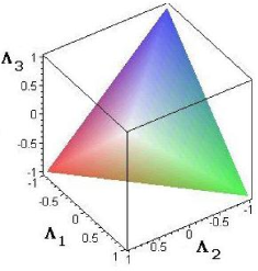
Figure 1: Geometric representation of PM versus CPM for the Bloch equations. All points of the unit cube represent positive maps. Points inside the tetrahedron are completely positive maps, given by the conditions (IV).

The Bloch inequalities (IV) lead to certain restrictions on the damping constants in the Bloch equations. For purely exponential character of the $\Lambda_{i}$, these conditions lead to a simpler relation involving only lifetimes. In this case each component of the Bloch vector can only decay according to Gorini (1976); Kimura (2002):

$$\begin{split}\frac{1}{T_{u}}\leq\frac{1}{T_{v}}+\frac{1}{T_{w}}\\ \frac{1}{T_{w}}\leq\frac{1}{T_{u}}+\frac{1}{T_{v}}\\ \frac{1}{T_{v}}\leq\frac{1}{T_{w}}+\frac{1}{T_{u}}.\end{split}$$ (24)

The condition of complete positivity leads to a set of Bloch inequalities for the phenomenological lifetimes that must be satisfied. This explains the well-known phenomenon in nuclear magnetic resonance whereby the inverse transverse relaxation time is always less than or equal to twice the inverse longitudinal relaxation time.

It is instructive to see how the violation of the Bloch inequalities (24) is reflected in the general conditions (IV). In order to show this, we have depicted in Fig. 2 the four conditions (IV) as a function of time for two different selections of the damping parameters. A function exceeding the straight line at the value one is not a CPM, because it violates the Bloch inequalities. Note that the case describe on the left figure is a PM that is not a CPM for all times, while the case on the right figure describes a CPM for all times.

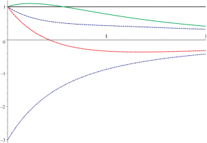
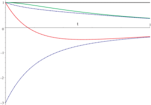
Figure 2: Plots of the four conditions (IV) as a function of time $t$. The left figure corresponds to $\frac{1}{T_{u}}=6,\frac{1}{T_{v}}=3,\frac{1}{T_{w}}=1$. The right figure corresponds to $\frac{1}{T_{u}}=6,\frac{1}{T_{v}}=5,\frac{1}{T_{w}}=1$. All values are in arbitrary units. We see that the figure on the left is not a CMP, because the Bloch inequalities (24) are violated.

Application of the Bloch inequalities to the case of squeezed noise given by Eqs. (6) leads to the condition $N+\frac{1}{2}\geq|M|$ gardiner1991 .

As a different example of a Bloch CMP generated by a noise, let us consider the Hamiltonian

$$H=x(t)\sigma_{x}+y(t)\sigma_{y}+z(t)\sigma_{z},$$ (25)

where $x(t)$, $y(t)$, and $z(t)$ are Gaussian random variables with

$$\begin{split}\langle x(t)x(s)\rangle&=\frac{\Gamma_{a}}{2}\delta(t-s)\\ \langle y(t)y(s)\rangle&=\frac{\Gamma_{b}}{2}\delta(t-s)\\ \langle z(t)z(s)\rangle&=\frac{\Gamma_{c}}{2}\delta(t-s).\end{split}$$ (26)

Note that the white noise correlation has the form $\langle a(t)a(s)\rangle=2D_{a}\delta(t-s)$, where the diffusion coefficient is $D_{a}=\frac{\Gamma_{a}}{4}$. The same holds for the remaining noises.

After averaging over the random variables, the Bloch vector will transform by exponentiating the following matrix:

$$\left(\begin{array}[]{ccc}\Gamma_{b}+\Gamma_{c}&0&0\\ 0&\Gamma_{a}+\Gamma_{c}&0\\ 0&0&\Gamma_{a}+\Gamma_{b}\end{array}\right).$$ (27)

As a result we obtain three different lifetimes given by the following relations:

$$\frac{1}{T_{u}}=\Gamma_{b}+\Gamma_{c},\hskip 7.22743pt\frac{1}{T_{v}}=\Gamma_{a}+\Gamma_{c},\hskip 7.22743pt\frac{1}{T_{w}}=\Gamma_{a}+\Gamma_{b}.$$ (28)

It is easy to verify that for positive diffusion coefficients these lifetimes always satisfy the Bloch inequalities (24) i.e., are always generating completely positive maps of the Bloch vector. An analysis of other cases in which there are three phenomenological decay rates can be found in Ref. Daffer (2003).

V Markovian Bloch Map

The Bloch equations with Gaussian white noise discussed in the previous section are just an example of a general class of Markovian completely positive maps. The general quantum Markovian master equation for the system density operator can be written in terms of the Gorini-Kossakowski-Sudarshan generator Gorini (1976); Kossakowski (1972); Lindblad (1976)

$$L\rho=-i[H,\rho]+\mathcal{L}\rho,$$ (29)

where the Lindblad superoperator may be written as

$$\mathcal{L}\rho=\frac{1}{2}\sum^{n^{2}-1}_{i,j=1}c_{ij}\{[F_{i},\rho F^{\dagger}_{j}]+[F_{i}\rho,F^{\dagger}_{j}]\}$$ (30)

for $\rho\in\mathcal{M}_{n}$ ($\mathcal{M}_{n}$ denotes the set of $n\times n$ complex matrices), where $H=H^{\dagger},\textrm{Tr}\{H\}=0,\textrm{Tr}(F_{i})=0,\textrm{Tr}\{F^{\dagger}_{i}F_{j}\}=\delta_{ij},$ and $(c_{ij})$ is a complex positive semidefinite matrix.

The expression in Eq. (29) has been shown to generate a dynamical semigroup Alicki (1987) that has the following properties:

$$(i) \parallel\Phi_{t}\rho\parallel_{1}=\parallel\rho\parallel_{1}\forall\hskip 3.61371pt\rho\in V_{1}^{+}(\mathcal{H}),\hskip 3.61371ptt\geq 0,$$

$$(ii) \Phi_{t}\otimes I_{n}\geq 0\hskip 3.61371pt\forall\hskip 3.61371ptn\in\textrm{Z}_{+},$$

$$(iii) \textrm{lim}_{t\downarrow 0}\hskip 3.61371pt\Phi_{t}=I,$$

$$(iv) \Phi_{t}\Phi_{s}=\Phi_{t+s},\hskip 3.61371ptt,s\geq 0.$$

Property $(i)$ states that the map is trace-preserving for all positive operators, which form a positive cone $V_{1}^{+}(\mathcal{H})$. $\parallel\cdot\parallel_{1}$ denotes the trace norm in the space of linear operators on the Hilbert space $\mathcal{H}$. The definition of complete positivity is given by property $(ii)$. We have already encountered this property in Eq. (18). The third property is a statement regarding continuity. The map $\Phi$ is continuous from above and approaches the identity superoperator. Property $(iv)$ is the essence of the semigroup property. It states that applying the map from time 0 to time $s$ and then applying the map from time $s$ to time $t$ is equivalent to applying the map from time 0 to time $t+s$. Obviously, exponential functions have this property.

In the following we will show that such Markovian maps can be conveniently written in terms of a damping basis. The map $\Phi$ can be written in the general form

$$\Phi(\bullet)=\sum_{i}\Lambda_{i}\textrm{Tr}\{L^{\dagger}_{i}\bullet\}R_{i},$$ (32)

where $L_{i}$ and $R_{i}$ are left and right eigenoperators, which form a damping basis Briegel (1993). $L_{i}$ is the operator dual to $R_{i}$ that satisfies the duality relation

$$\textrm{Tr}\{L_{i}R_{j}\}=\delta_{ij}.$$ (33)

This is a complete, orthogonal basis with which to expand the density operator at any time.

This basis is obtained by finding the eigenoperators of the eigenvalue equation. The right eigenoperators satisfy

$${\cal L}R_{i}=R_{i}\lambda,$$ (34)

while the left eigenoperators satisfy the dual eigenvalue equation

$$L_{i}{\cal L}=\lambda L_{i}.$$ (35)

Both $L_{i}$ and $R_{i}$ have the same eigenvalues.

If we use the eigenoperators $R_{i}$ of Eq. (34) with corresponding eigenvalues $\lambda_{i}$, then once the initial state is known

$$\rho(0)=\sum_{i}\textrm{Tr}\{L_{i}\rho(0)\}R_{i},$$ (36)

the state of the system at any later time can be found through

$$\rho(t)=e^{{\cal L}t}\rho(0)=\sum_{i}\textrm{Tr}\{L_{i}\rho(0)\}\Lambda_{i}R_{i}$$ (37)

$$=\sum_{i}\textrm{Tr}\{R_{i}\rho(0)\}\Lambda_{i}L_{i},$$

where $\Lambda_{i}$ are functions of both time and the eigenvalues $\lambda_{i}$. An arbitrary positive map must have the contractions $|\Lambda_{i}|\leq 1$.

This method is a simple way of finding the density operator for a given ${\cal L}$ for all times. The solution of the left and right eigenvalue equations yields a set of eigenvalues and eigensolutions: $\{\lambda_{i},L_{i},R_{i}\}.$ Once the damping basis is obtained, it can be used to expand the density operator.

As an example let us investigate a stochastic model of a depolarizing channel with white noise. As a simple example, we will consider Bloch Eqs.(II) that have the following phenomenological decay constants:

$$\frac{1}{T_{1}}=0,\hskip 14.45377pt\frac{1}{T_{2}}=D,\hskip 14.45377pt\frac{1}{T_{3}}=0,\hskip 14.45377ptw_{eq}=0.$$ (38)

This describes the process of phase randomization of the atomic dipole caused by atomic collisions. This leads to equal damping for the $u$ and $v$ components of the Bloch vector with contractions that depend on the parameter $D$ due to collisions. Setting both $\Omega$ and $\Delta$ equal to zero, the Lindbladian for this system is

$$\mathcal{L}\bullet=-D[\sigma_{3},[\sigma_{3},\bullet]].$$ (39)

$\mathcal{L}$ is the generator of the dissipative dynamics

$$\Phi(\rho)=e^{t\mathcal{L}}\rho(0)$$ (40)

and always generates a completely positive dynamical semigroup. The decay constant is a scalar parameter that arises after tracing or averaging over the environment degrees of freedom. The environment could be a quantum reservoir or a classically fluctuating external system. The von Neumann equation

$$\dot{\rho}=-iz(t)[\sigma_{3},\rho]$$ (41)

for system and environment, containing a stochastic variable $z(t)$, can be averaged over the noise exactly to obtain Eq. (39). The noise leads to bit flip errors in the system.

The damping basis for the bit flip Lindblad equation is given in Pauli basis by

$$R_{\alpha}=\frac{1}{\sqrt{2}}\sigma_{\alpha}\,.$$ (42)

The left eigenoperators are identical to the right eigenoperators because the Pauli operators are self-dual. The damping eigenvalues are given by

$$\lambda_{0}=0,\hskip 7.22743pt\lambda_{1}=-4D,\hskip 7.22743pt\lambda_{2}=-4D,\hskip 7.22743pt\lambda_{3}=0.$$ (43)

The time dependent functions $\Lambda_{i}$ become

$$\Lambda_{0}=1,\hskip 7.22743pt\Lambda_{1}=e^{-4Dt},\hskip 7.22743pt\Lambda_{2}=e^{-4Dt},\hskip 7.22743pt\Lambda_{3}=1.$$ (44)

The reduced dynamics describe dissipation of the system due to the coupling of it with the environment. The dissipation is in the form of pure damping. In the Bloch equations, this leads to phenomenological decay constants

$$\frac{1}{T_{2}}=\frac{1}{T_{u}}=\frac{1}{T_{v}}=4D,\hskip 14.45377pt\frac{1}{T_{1}}=\frac{1}{T_{w}}=0$$ (45)

for each component of the Bloch vector. The inversion, given by the $w$ component undergoes no damping. The two orthogonal components $u$ and $v$ undergo equal damping.

The bit flip error equation results in a completely positive, trace-preserving map. Thus, there exists a set of Kraus operators, which can be used to write the map as a decomposition in terms of these operators. Two Kraus operators can be used to write the decomposition as

$$\Phi(\rho)=K_{0}\rho K^{\dagger}_{0}+K_{3}\rho K_{3}^{\dagger},$$ (46)

with Kraus operators explicitly given by

$$K_{0}=\sqrt{\frac{1+e^{-4Dt}}{2}}\;I,K_{3}=\sqrt{\frac{1-e^{-4Dt}}{2}}\;\sigma_{3}.$$ (47)

It is easy to show that these operators are normalized

$$K_{0}^{\dagger}K_{0}+K_{3}^{\dagger}K_{3}=I,$$ (48)

thus producing a trace-preserving completely positive map.

VI Non-Markovian Bloch Map

The damping basis method can be applied to non-Markovian Bloch maps. Such maps occur for example in a depolarizing channel with colored noise. A bit flip error equation that does not rely on the white noise assumption can be derived. This is achieved by assuming the environment has correlations that are not of the form of a delta-function, resulting in what is called colored noise. The master equation is no longer of the Lindblad type; instead, it contains a memory kernel operator leading to a master equation of the general form

$$\dot{\rho}=K\mathcal{L}\rho,$$ (49)

where $K$ is an integral operator that depends on time of the form $K\phi=\int_{0}^{t}k(t-t^{\prime})\phi(t^{\prime})\textrm{d}t^{\prime}$. The kernel function $k(t-t^{\prime})$ is a well-behaved, continuous function that determines the type of memory in the physical problem. The solution to the master equation can be found by taking the Laplace transform

$$s\tilde{\rho}(s)-\rho(0)=\tilde{K}(s)\mathcal{L}\tilde{\rho}(s),$$ (50)

determining the poles, and inverting the equation in the standard way.

To illustrate this class of master equations, the exponential kernel function

$$k(s,t)=e^{-\frac{|t-s|}{\tau}}$$ (51)

is used. Consider the Hamiltonian $H=z(t)\sigma_{3}$ with a random telegraph signal (RTS) random variable $z(t)=a(-1)^{n(t)}.$ The random variable $n(t)$ has a Poisson distribution with a mean equal to $t/2\tau$, while $a$ is an independent coin-flip random variable VanKampen (1981). The equation of motion for the density operator is given by the commutator

$$\dot{\rho}=-i[H,\rho]=-iz(t)[\sigma_{3},\rho].$$ (52)

Taking the ensemble average over the random variables $z(t)$ leads to an equation of motion for the average density operator Wodkiewicz (1984)

$$\dot{\rho}=-a^{2}\int_{0}^{t}e^{-\frac{t-s}{\tau}}[\sigma_{3},[\sigma_{3},\rho(s)]]\textrm{d}s.$$ (53)

The brackets denoting the ensemble average are omitted and it should be understood that we are considering the average density operator. The master equation for the bit flip error with an exponential memory kernel is exact.

The damping basis diagonalizes the equation. This leads to a single equation, for the two nontrivial components, that has the following form:

$$\frac{\textrm{d}}{\textrm{d}t}c(t)=-4a^{2}\int_{0}^{t}\textrm{d}se^{-\frac{|t-s|}{\tau}}c(s)\textrm{d}s.$$ (54)

Taking a derivative gives a second order differential equation

$$\frac{\textrm{d}^{2}}{\textrm{d}t^{2}}c(t)+\frac{1}{\tau}\frac{\textrm{d}}{\textrm{d}t}c(t)+4a^{2}c(t)=0\,.$$ (55)

The function $c(t)$ is the solution to a damped harmonic oscillator equation of motion

$$c(t)=e^{-\frac{t}{2\tau}}\left(\cos(\Omega t)+\frac{\sin(\Omega t)}{2\Omega\tau}\right),$$ (56)

where $\Omega=\sqrt{4a^{2}-\frac{1}{4\tau^{2}}}$ and $c(0)=1$.

The image of this random telegraph signal (RTS) map is similar to that of a depolarizing channel with white noise. The transformation given by Eq. (10) for this noise is

$${\cal T}=\left(\begin{array}[]{cccc}1&0&0&0\\ 0&c(t)&0&0\\ 0&0&c(t)&0\\ 0&0&0&1\end{array}\right),$$ (57)

which has the same form as the depolarizing channel. Notice that there are no translations of the Bloch vector and

$$\Lambda(t)=\Lambda_{1}=\Lambda_{2}=c(t),\ \ \Lambda_{2}=c(t),\ \ \mathrm{and}\ \ \Lambda_{3}=1.$$ (58)

The depolarizing channel with white noise has simple contractions so that $c(t)$ is an exponential function. This is a property of white noise. The RTS channel has colored noise leading to a nonexponential function for $\Lambda(t)$. Rather, it contains oscillating terms with an exponential envelope. A power series expansion gives

$$\Lambda(\nu)=1-2a^{2}t^{2}+O(t)^{3}\,,$$ (59)

which shows that the linear term in $t$ is missing. Thus, the standard white noise diffusion term vanishes. This is in contrast to the Markovian case, where the functions are purely exponential functions in time with parameters defining the characteristic lifetimes. This is a general property of the memory kernel and a fundamental difference between white noise and colored noise. The white noise limit can be recovered from (58) with a singular limit of $\tau\rightarrow 0$ and $\gamma=4a^{2}=\mathrm{const}$. In such a white noise limit $\Lambda_{\mathrm{wn}}=e^{-\gamma t}$.

In terms of the dimensionless time $\nu=t/2\tau$ we can write $\Lambda(\nu)=e^{-\nu}(\cos(\mu\nu)+\frac{\sin{(\mu\nu)}}{\mu})$, with $\mu=\sqrt{(4a\tau)^{2}-1}$. The function $\Lambda(\nu)$ has two regimes – pure damping and damped oscillations. The fluctuation parameter, given by the product $a\tau$, determines the behavior of the solution. When $0\leq a\tau<1/4$ the solution is described by damping. The frequency $\mu$ is imaginary with magnitude less than unity. When $a\tau=1/4$ the function $\Lambda(\nu)=e^{-\nu}(1-\nu)$ is unity at the initial time and approaches zero as time approaches infinity. In addition to pure damping, damped harmonic oscillations in the interval $[-1,+1]$ exist in the regime $a\tau>1/4$.

The Kraus operators for the RTS channel are similar to those for the depolarizing channel. The non-Markovian Bloch map can be defined as

$$\begin{split}\Phi(\rho)&=K_{1}^{\dagger}\rho K_{1}+K_{2}^{\dagger}\rho K_{2}\\ &=\frac{1}{2}[1+\Lambda(t)]\,\rho+\frac{1}{2}[1-\Lambda(t)]\,\sigma_{3}\rho\sigma_{3}.\end{split}$$ (60)

The Bloch sphere evolves into an ellipsoid according to the equation

$$\left(\frac{u}{\Lambda(t)}\right)^{2}+\left(\frac{v}{\Lambda(t)}\right)^{2}+w^{2}=1.$$ (61)

Unlike the exponential damped solution for white noise, the function can take on negative values and is bounded between $\pm 1$.

VII Noise and separability

The maximally entangled Bell state can be used to test if an arbitrary map for qubits is completely positive. The initial entangled state for two qubits is given by a positive semidefinite density operator. If only one qubit of the joint state is subjected to noise, the joint state must also be described by a positive semidefinite density operator for all time. For $n$-level systems, positivity of the maximally entangled $n^{2}$-level state implies that the map for the $n$-level part of the state is completely positive.

The maximally entangled two qubit state can also be used to address the issue of separability. The partial transposition map is an example of a map that is positive but not completely positive. The partial transposition map applied to an entangled $n^{2}$ state involves performing the transpose operation on one half of the state, while performing the identity operation on the other part of the state. Note that the partial transposition map is not a continuous map connected to the identity superoperator. Although the initial entangled state is described by a positive semidefinite density operator, the resulting transposed state can be negative. Using the Peres criterion of the positivity of the partial transpose, one can determine when the state becomes separable peres1996 . A necessary and sufficient condition for the output state to be nonseparable is that the partial transpose map be negative horodecki1996 . To check the positivity of the partial transpose it suffices to examine the eigenvalues of the operator given by

$$\widetilde{\Phi}(\rho_{AB})=\mathbf{1}_{A}\otimes\mathrm{T}_{B}[\Phi(\rho_{AB})]$$ (62)

where $\mathrm{T}_{B}$ denotes the transpose of the state of Bob’s qubit. The dynamical map $\Phi$ is first applied to the maximally entangled state in the following way: $\Phi(\rho_{AB})=I_{A}\otimes\Phi_{B}[\rho_{AB}]$. The transposition map acts on one half of the entangled state and the output state is given by $\widetilde{\Phi}(\rho_{AB})$ in Eq. (62).

The four eigenvalues of the partial transpose matrix for the bit flip error are

$$\begin{split}e_{1}=e_{2}=\frac{1}{2},\hskip 14.45377pte_{3}=-\frac{\Lambda(t)}{2},\hskip 14.45377pte_{4}=\frac{\Lambda(t)}{2}\,.\end{split}$$ (63)

¿From this relation we conclude that such a state is separable if and only if $\Lambda(t)=0$. This shows that in the limit of Markovian dynamics, the separability is reached only in the asymptotic limit of $t\rightarrow\infty$. The situation is remarkably different for a non-Markovian map. In Figure 3 we have depicted the separability condition as a function of the color of the noise, characterized by the parameter $\tau$.

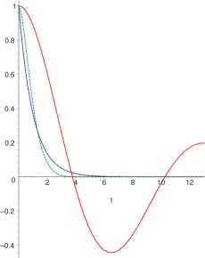
Figure 3: Plots of non-Markovian $\Lambda(t)$ and $\tau=4$, (solid line), $\tau=0.3$ (dot-line), white noise case $\tau=0$ (dash-line). All plots in arbitrary units with $\gamma=1$. The state becomes separable for $\Lambda(t)=0$.

VIII Conclusion

The Bloch equations are well-known to physicists working in the field of nuclear resonance or quantum optics. These equations have been widely used in quantum information theory to describe the dissipation of various quantum channels for qubits. The original Bloch equations have been derived on a purely phenomenological ground, and phenomenological damping constants have been introduced. We have shown that the physical consequences of a quantum mechanical description of dissipation leads to complete positivity of the Bloch maps. The condition that these maps are CPM, implies a set of Bloch equations for the generalized eigenvalues of the damping matrix. In the case of pure Markovian dissipations these Bloch equations can be reduced to simple inequalities for the various lifetimes characterizing the qubit. We have shown that this approach can be extended to non-Markovian dynamics. In this case the Bloch inequalities involve time-dependent eigenvalues of the generalized damping matrices. We have illustrated our points with examples of Markovian and non-Markovian depolarizing channels for qubits. We have shown a fundamental difference in the separability properties of correlated qubits in such channels.