Polarization-sensitive quantum-optical coherence tomography

Abstract

We set forth a polarization-sensitive quantum-optical coherence tomography (PS-QOCT) technique that provides axial optical sectioning with polarization-sensitive capabilities. The technique provides a means for determining information about the optical path length between isotropic reflecting surfaces, the relative magnitude of the reflectance from each interface, the birefringence of the interstitial material, and the orientation of the optical axis of the sample. PS-QOCT is immune to sample dispersion and therefore permits measurements to be made at depths greater than those accessible via ordinary optical coherence tomography. We also provide a general Jones matrix theory for analyzing PS-QOCT systems and outline an experimental procedure for carrying out such measurements.

I INTRODUCTION

Optical coherence tomography (OCT) has become a well-established imaging technique Huang et al. (1991); Fujimoto et al. (1995); Fercher (1996); Schmidt (1999) with applications in ophthalmology Hee et al. (1995), intravascular measurements Brezinski and Fujimoto (1999); Fujimoto et al. (1999), and dermatology Welzel (2001). It is a form of range-finding that makes use of the second-order coherence properties of a classical optical source to effectively section a reflective sample with a resolution governed by the coherence length of the source. OCT therefore makes use of sources of short coherence length (and consequently broad spectrum), such as superluminescent diodes (SLDs) and ultrashort-pulsed lasers. As broad bandwidth sources are developed to improve the resolution of OCT techniques, material dispersion has become more pronounced. The deleterious effects of dispersion broadening limits the achievable resolution as has been recently emphasized Drexler et al. (2001).

To further improve the sensitivity of OCT, techniques for handling dispersion must be implemented. In the particular case of ophthalmologic imaging, one of the most important applications of OCT, the retinal structure is located behind a comparatively large body of dispersive ocular media Hitzenberger et al. (1999). Dispersion increases the width of the coherence envelope of the probe beam and results in a reduction in axial resolution and fringe visibility Hitzenberger et al. (2002). Current techniques for depth-dependent dispersion compensation include the use of dispersion-compensating elements in the optical set-up Hitzenberger et al. (1999); Smith et al. (2002) or employ a posteriori numerical methods Fercher et al. (2001, 2002). For these techniques to work, however, the object dispersion must be known and well characterized so that the appropriate optical element or numerical algorithm can be implemented.

Over the past several decades, a number of non-classical (quantum) sources of light have been developed Teich and Saleh (1988, 1990) and it is natural to inquire whether making use of any of these sources might be advantageous for tomographic imaging. An example of such a nonclassical source is spontaneous parametric down-conversion (SPDC) Klyshko (1967); Harris et al. (1967); Giallorenzi and Tang (1968); Kleinman (1968); Burnham and Weinberg (1970); Larchuk et al. (1995a), a nonlinear process that produces entangled beams of light. This source, which is broadband, has been utilized to demonstrate a number of interference effects that cannot be observed using traditional classical sources of light. We make use of this unique feature in quantum-optical coherence tomography (QOCT) Abouraddy et al. (2002a), where fourth-order interference is used to provide range measurements analogous to those currently obtained using classical OCT, but with the added advantage of even-order dispersion cancellation Franson (1992); Steinberg et al. (1992); Larchuk et al. (1995b). We have recently demonstrated the dispersion immunity of these tomographic measurements in comparison to standard optical coherence tomography techniques Nasr et al. (2003).

In this paper, we present a method for polarization-sensitive QOCT (PS-QOCT) measurements, where one can detect a change in the polarization state of light reflected from a layered sample Hee et al. (1992). This state change arises from scattering and birefringence in the sample and is enhanced in specimens that have an organized linear structure. Tissue that contains a high content of collagen or other elastin fibers, such as tendons, muscle, nerve, or cartilage, are particularly suited to polarization-sensitive measurements de Boer et al. (1999). A variation in birefringence can be indicative of a change in functionality, integrity, or viability of biological tissue.

II GENERAL MATRIX THEORY FOR PS-QOCT

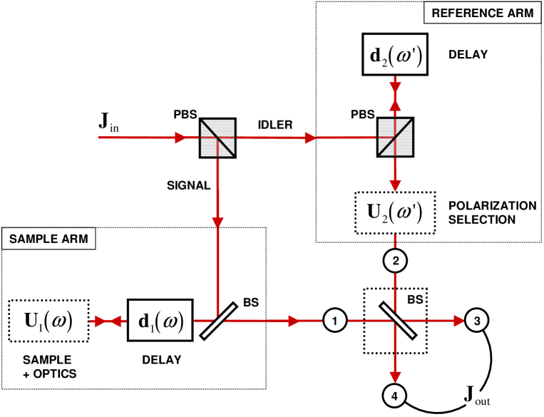
Figure 1: Conceptual diagram of polarization-sensitive quantum-optical coherence tomography (PS-QOCT). The system is based on a Mach-Zehnder interferometer in which twin photons from SPDC, represented by the vector $\rm{{\bf J}_{in}}$, are separated into two arms at a polarizing beam splitter (PBS). The signal photon at angular frequency $\omega$ travels in the sample arm and experiences a path delay $\rm{\bf d}_{1}$ as well as an arbitrary polarization rotation described by $\rm{\bf U}_{1}$. The reference arm contains the idler photon at angular frequency $\omega^{\prime}$ which experiences a path delay $\rm{\bf d}_{2}$ and a user-selected polarization rotation $\rm{\bf U}_{2}$. Paths ➀ and ➁ impinge on a final beam splitter (BS) which mixes the spatial/polarization modes into paths ➂ and ➃. $\rm{{\bf J}_{out}}$ represents the final twin-photon Jones vector from which the fields at the detectors and the final coincidence rate are computed.

We present the theory for PS-QOCT according to the simplified diagram for an experimental setup given in Fig. 1. Using a Jones-matrix formalism similar to that in Ref. Abouraddy et al. (2002b), we start by defining a twin-photon Jones vector $\rm{{\bf J}_{in}}$

$$\rm{{\bf J}_{in}}=\begin{bmatrix}{\hat{a}}_{\rm s}(\omega)\,{\bf e}_{\rm s}\\ {\hat{a}}_{\rm i}(\omega^{\prime})\,{\bf e}_{\rm i}\end{bmatrix},$$ (1)

where ${\hat{a}}_{\rm s}(\omega)$ and ${\hat{a}}_{\rm i}(\omega^{\prime})$ are the annihilation operators for the signal-frequency mode $\omega$ and the idler-frequency mode $\omega^{\prime}$, respectively. The vectorial polarization information for the signal and idler field modes are contained in ${\bf e}_{j}$, ($j={\rm s,\,i}$). For example, if we utilize collinear type-II SPDC from a second-order nonlinear crystal (NLC) to generate a pair of orthogonally polarized photons, the ${\bf e}_{j}$ reduce to the familiar Jones vectors:

$${\bf e}_{\rm s} = \genfrac{[}{]}{0.0pt}{}{1}{0}\quad\quad{\rm(vertical)}$$

$${\bf e}_{\rm i} = \genfrac{[}{]}{0.0pt}{}{0}{1}\quad\quad{\rm(horizontal)}$$ (2)

for signal and idler, respectively.

The twin photons collinearly impinge on the input port of a polarizing beam splitter (PBS) from which the signal photon is reflected into the sample arm and the idler photon is transmitted into the reference arm. We assume that the polarization in each arm is independent of that in the other arm until the final beam splitter. We also assume that all optical elements within the interferometer are linear and deterministic.

The delay accumulated by the signal and idler beams in each path is represented by the $2\times 2$ matrix

$$\rm{\bf D}=\begin{bmatrix}\rm{\bf d}_{1}(\omega)&0\\ 0&\rm{\bf d}_{2}(\omega^{\prime})\end{bmatrix},$$ (3)

where $\rm{\bf d_{1}}(\omega)$ and $\rm{\bf d_{2}}(\omega^{\prime})$ represent the Jones matrices that describe the delay for the sample and reference arms, respectively. The polarization state in each arm is represented by the matrix

$$\rm{\bf U}=\begin{bmatrix}\rm{\bf U}_{1}(\omega)&0\\ 0&\rm{\bf U}_{2}(\omega^{\prime})\end{bmatrix}.$$ (4)

In the experimental realization of PS-QOCT, the matrix $\rm{\bf U}_{1}(\omega)$ represents the properties of the sample plus any other polarization elements in the sample arm, whereas $\rm{\bf U}_{2}(\omega^{\prime})$ represents the user-selected polarization state in the reference arm.

The mixing of the polarizations from each path, which occurs at the final beam splitter, is represented by the transformation matrix

$$\rm{{\bf T}_{BS}}=\begin{bmatrix}\rm{\bf T}_{31}&\rm{\bf T}_{32}\\ \rm{\bf T}_{41}&\rm{\bf T}_{42}\end{bmatrix},$$ (5)

where each element ${\rm\bf T}_{kl}$ ($k=$ 3, 4 and $l=$ 1, 2) is a $2\times 2$ matrix that represents the mixing of independent polarization modes from the input paths ➀ and ➁ prior to detection in paths ➂ and ➃. For example, $\rm{\bf T}_{31}$ is the Jones matrix that represents the transformation of input spatial mode 1 into output spatial mode 3.

The Jones vector $\rm{{\bf J}_{out}}$ that describes the field operators at the output of the final beam splitter, can be computed from the product of the previously defined matrices in Eqs. (3) – (5) as

$$\rm{{\bf J}_{out}}=\rm{{\bf T}_{BS}}\,\rm{\bf U}\,\rm{\bf D}\,\rm{{\bf J}_{in}}=\begin{bmatrix}\rm{\bf T}_{31}\rm{\bf U}_{1}\rm{\bf d}_{1}&\rm{\bf T}_{32}\rm{\bf U}_{2}\rm{\bf d}_{2}\\ \rm{\bf T}_{41}\rm{\bf U}_{1}\rm{\bf d}_{1}&\rm{\bf T}_{42}\rm{\bf U}_{2}\rm{\bf d}_{2}\end{bmatrix}\,\rm{{\bf J}_{in}}.$$ (6)

¿From this equation, the fields in paths ➂ and ➃ arriving at each of the two detectors can be written in the time domain as

$${\hat{\bf E}}^{(+)}_{3}(t_{3})=\int{\rm d}\omega\,{\rm e}^{-{\rm i}\omega t_{3}}\,{\hat{a}}_{\rm s}(\omega)\,{\bf e}_{3{\rm s}}+\int{\rm d}\omega^{\prime}\,{\rm e}^{-{\rm i}\omega^{\prime}t_{3}}\,{\hat{a}}_{\rm i}(\omega^{\prime})\,{\bf e}_{3{\rm i}}$$ (7)

$${\hat{\bf E}}^{(+)}_{4}(t_{4})=\int{\rm d}\omega\,{\rm e}^{-{\rm i}\omega t_{4}}\,{\hat{a}}_{\rm s}(\omega)\,{\bf e}_{4{\rm s}}+\int{\rm d}\omega^{\prime}\,{\rm e}^{-{\rm i}\omega^{\prime}t_{4}}\,{\hat{a}}_{\rm i}(\omega^{\prime})\,{\bf e}_{4{\rm i}},$$ (8)

where

$${\bf e}_{3{\rm s}}={\bf T}_{31}\,{\bf U}_{1}\,{\bf d}_{1}\,{\bf e}_{\rm s}\hskip 85.35826pt{\bf e}_{3{\rm i}}={\bf T}_{32}\,{\bf U}_{2}\,{\bf d}_{2}\,{\bf e}_{\rm i}$$

$${\bf e}_{4{\rm s}}={\bf T}_{41}\,{\bf U}_{1}\,{\bf d}_{1}\,{\bf e}_{\rm s}\hskip 85.35826pt{\bf e}_{4{\rm i}}={\bf T}_{42}\,{\bf U}_{2}\,{\bf d}_{2}\,{\bf e}_{\rm i}$$ (9)

describes each of the transformations of the signal and idler polarizations that contribute to the final fields in ➂ and ➃ at the detectors.

¿From the field at each of the detectors, the two-photon amplitude can be written as

$$A_{jk}(t_{3},t_{4})=\langle 0|{\hat{E}}^{(+)}_{3j}(t_{3}){\hat{E}}^{(+)}_{4k}(t_{4})|\Psi\rangle,$$ (10)

where $j$ and $k$ represent two orthogonal polarization bases such as horizontal/vertical (H/V), right/left circular (R/L), or (45^∘/-45^∘). The ket $|\Psi\rangle$ represents the two-photon state at the output of the nonlinear crystal, defined as

$$|\Psi\rangle=\int{\rm d}\Omega\,\Phi(\Omega)\,\hat{a}^{\dagger}_{\rm s}(\omega_{0}+\Omega)\,\hat{a}^{\dagger}_{\rm i}(\omega_{0}-\Omega)|0\rangle,$$ (11)

where $\Phi(\Omega)$ is the state function Di Giuseppe et al. (2002) that governs the spatio-temporal properties of the signal and idler photons at angular frequency $\omega_{0}\pm\Omega$. The state function is given by $\Phi(\Omega)=L\,{\rm sinc}[\Delta k_{z}(\Omega)L/2]$, where $L$ is the crystal length and $\Delta k_{z}(\Omega)$ is the wave-vector mismatch in the $z$- or phase-matching direction. If the state function $\Phi(\Omega)$ is symmetric about the center frequency or $\Phi(-\Omega)=\Phi(\Omega)$, the SPDC spectrum becomes $|\Phi(\Omega)|^{2}$.

We assume that the detection apparatus is slow and independent of polarization so that the final coincidence rate $R$ is computed as the magnitude-square of the two-photon amplitude summed over each polarization mode, integrated over time:

$$R=\int dt_{3}\int dt_{4}\sum_{j}\sum_{k}|A_{jk}(t_{3},t_{4})|^{2}.$$ (12)

III SIMPLIFIED CONFIGURATION FOR PS-QOCT

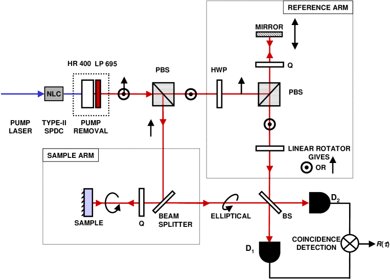
Figure 2: Possible implementation of polarization-sensitive quantum-optical coherence tomography (PS-QOCT). A narrow-band pump laser at a wavelength of 400 nm pumps a 1.5-mm-thick $\beta$-barium borate (BBO) nonlinear crystal (NLC) oriented for type-II, collinear SPDC with a center wavelength of 800 nm. The pump beam is removed from the SDPC by use of a highly reflective mirror (HR 400) centered at the pump wavelength concatenated with a long pass filter (LP 695). The vertical and horizontal components in the SPDC beam are separated by a polarizing beam splitter (PBS) into the reference arm and sample arm of a Mach-Zehnder interferometer. The reference arm consists of a variable path-length delay comprised of a half-wave plate (HWP), a second polarizing beam splitter (PBS), a quarter-wave plate (Q), and a translational mirror. The final polarization of the reference beam (indicated as $\odot$) can be oriented to either vertical or horizontal by a linear rotator prior to the final beam splitter (BS). The sample arm consists of a beam splitter and a quarter-wave plate (Q) so that circularly polarized light is normally incident on the sample. The back-reflected light from the sample, which in general has elliptical polarization, mixes with the delayed reference beam at the final beam splitter (BS). The outputs from the BS are directed to two single-photon counting detectors. The coincidence rate $R(\tau)$ for photons arriving at the two detectors, as a function of the path-length delay $c\tau$, are recorded in a time window determined by a coincidence-counting detection circuit (indicated as $\otimes$).

It is now useful to consider a specific experimental configuration from which we can define expressions for the Jones matrices in Eqs. (3) – (5) and calculate the quantum interferogram. One particular experimental configuration for PS-QOCT is based on the Mach-Zehnder interferometer and is shown in Fig. 2.

The elements of the Jones matrix in Eq. (3), representing the delay in each path, are given simply by ${\bf d}_{1}(\omega)={\bf I}\,{\rm e}^{{\rm i}\omega z_{\rm s}/c}$ and ${\bf d}_{2}(\omega^{\prime})={\bf I}\,{\rm e}^{{\rm i}\omega^{\prime}z_{\rm r}/c}$, where ${\bf I}$ is the identity matrix, $c$ is the speed of light in the medium, and $z_{\rm s}$, $z_{\rm r}$ are the path lengths in the sample and reference arms, respectively. We define a path-delay difference $\tau=(z_{\rm r}-z_{\rm s})/c$ between the reference and sample arms that becomes our experimental parameter in the final expression for the measured coincidence rate $R(\tau)$. We assume that the final beam splitter faithfully transmits and reflects each input polarization mode. The elements of ${\bf T}_{\rm BS}$ in Eq. (5) thus become ${\bf T}_{31}={\bf T}^{{\dagger}}_{42}=t\,{\bf I}$ and ${\bf T}_{32}=-{\bf T}^{{\dagger}}_{41}=r^{\ast}\,{\bf I}$, where ${\dagger}$ designates a matrix transpose and conjugation, and $t$ and $r$ represent the amplitude transmittance and reflectance of the beam splitter, respectively.

Without having to specify the elements of ${\bf U}$ in Eq. (4), an expression for the measured coincidence rate as a function of the path-delay difference $\tau$ is calculated to be

$$R(\tau)\propto\Lambda_{0}-{\mathcal{V}}_{\rm BS}\,{\rm Re}\left[\Lambda(2\tau)\right],$$ (13)

where $\Lambda_{0}$ and $\Lambda(\tau)$ are defined as

$$\Lambda_{0}=\int d\Omega\,|\Phi(\Omega)|^{2}\,[{\bf e}^{{\dagger}}_{\rm s}\,{\bf U}^{{\dagger}}_{1}(\omega_{0}+\Omega)\,{\bf U}_{1}(\omega_{0}+\Omega)\,{\bf e}_{\rm s}]\,({\bf e}^{{\dagger}}_{\rm i}\,{\bf U}^{{\dagger}}_{2}\,{\bf U}_{2}\,{\bf e}_{\rm i})$$ (14)

and

$$\Lambda({\tau})=\int d\Omega\,|\Phi(\Omega)|^{2}\,F(\omega_{0}+\Omega)\,F^{\ast}(\omega_{0}-\Omega)\,{\rm e}^{-{\rm i}\Omega\tau},$$ (15)

representing constant and varying contributions to the quantum interferogram, respectively. The function $F(\omega)$, which includes all of the sample properties, is given by

$$F(\omega)={\bf e}^{{\dagger}}_{\rm i}\,{\bf U}^{{\dagger}}_{2}\,{\bf U}_{1}(\omega)\,{\bf e}_{\rm s}.$$ (16)

The parameter ${\mathcal{V}}_{\rm BS}=2(|r|^{2}|t|^{2})/(|r|^{4}+|t|^{4})$ in Eq. (13) represents a visibility factor for a lossless beam splitter with arbitrary transmittance (${\mathcal{V}}_{\rm BS}=1$ when $|r|^{2}=|t|^{2}=1/2$). We assume that the optical elements in the reference arm are frequency independent across the bandwidth of the light-source spectrum. Equation (15) is a generalization of Eq. (8) in Ref. Abouraddy et al. (2002a), where the function $F$ contains polarization-dependent information about the sample.

It is clear from Eq. (15) that the sample is simultaneously probed at two frequencies, $\omega_{0}+\Omega$ and $\omega_{0}-\Omega$, and that for a frequency-entangled two-photon state such that produced by SPDC, even-order dispersion from the sample is cancelled in PS-QOCT. The effectiveness of even-order dispersion cancellation is related to the spectrum of the source used for SPDC. Since we assume a cw-pump source in Eq. (11), this leads to signal and idler photons that are exactly frequency anti-correlated. In this case, even-order dispersion cancellation is perfect. As the bandwidth of the SPDC pump source is increased, the requirements for exact frequency anti-correlation are relaxed and dispersion cancellation is degraded. It is apparent that the delay $\tau$ can be adjusted to target specific regions in the sample from which polarization information can be extracted by scanning the parameters of the user-selected polarization rotator $\rm{\bf U}_{2}$. This experimental method is similar to those used in quantum ellipsometry, as discussed in Ref. Abouraddy et al. (2002b).

In the following section, we consider a specific construct for Eq. (4) that defines the optics in the experimental setup represented in Fig. 2. Once we derive an expression valid for an arbitrary sample, we consider several special cases in an effort to understand the nature of the information contained in the quantum interferogram.

IV ROLE OF POLARIZATION IN PS-QOCT

To facilitate the description of PS-QOCT, we make use of the Pauli spin matrices

$$\mbox{\boldmath$\sigma$}_{1}=\left[\begin{array}[]{ccc}0&1\\ 1&0\end{array}\right]\hskip 56.9055pt\mbox{\boldmath$\sigma$}_{2}=\left[\begin{array}[]{ccc}0&-{\rm i}\\ {\rm i}&0\end{array}\right]\hskip 56.9055pt\mbox{\boldmath$\sigma$}_{3}=\left[\begin{array}[]{ccc}1&0\\ 0&-1\end{array}\right],$$ (17)

from which any 2 x 2 Hermitian matrix can be defined as ${\rm\bf A}=c_{0}\,{\rm\bf I}+{\bf c}\cdot{\bm{\sigma}}$, where ${\bf c}\equiv(\mbox{$c$}_{1},\mbox{$c$}_{2},\mbox{$c$}_{3})$, ${\bm{\sigma}}\equiv(\mbox{\boldmath$\sigma$}_{1},\mbox{\boldmath$\sigma$}_{2},\mbox{\boldmath$\sigma$}_{3})$, and ${\bf c}\cdot{\bm{\sigma}}$ denotes the scalar product of vectors ${\bf c}$ and ${\bm{\sigma}}$. We first define Eq. (4) for $N$ reflective layers, where each reflection is assumed to be isotropic, then consider the special cases of a single and double reflector.

IV.1 $N$ reflective layers

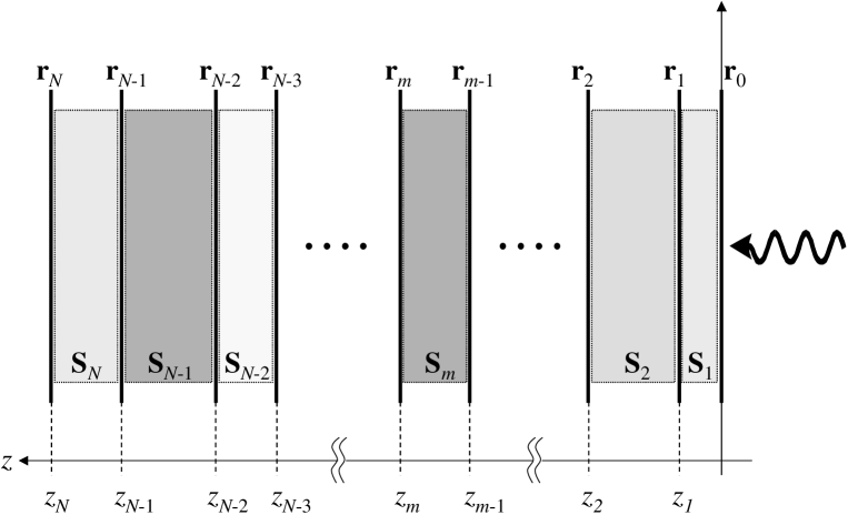
Figure 3: Sample comprised of $N$ reflective layers. The probe beam is incident at the right. Each interface at position $z_{m}$ is described by a reflectance matrix ${\rm{\bf r}}_{m}(\omega)$. The optical properties of the sample layers between interfaces are described by the Jones matrix ${\rm{\bf S}}_{m}$.

We begin with a sample comprised of $N$ reflective layers, each with an interface defined by a reflectance matrix ${\rm\bf r}_{m}(\omega)$, as shown in Fig. 3. The material properties of each layer are represented by a Jones matrix ${\rm\bf S}_{m}$ that is assumed to be deterministic. The Jones matrix ${\rm\bf S}_{m}$ is a product of: an average phase delay; rotation matrices ${\rm\bf R}_{m}$ to account for the orientation $\alpha_{m}$ of the fast axis of the sample with respect to the horizontal axis; and the Jones matrix ${\bf b}_{m}$ for a linear retarder with its fast axis oriented along the horizontal axis de Boer et al. (2001). If we ignore losses due to absorption, then for a single layer of thickness $d_{m}=(z_{m}-z_{m-1})$, the Jones matrix is given by

$${\bf S}_{m}(d_{m},\alpha_{m},\omega) = {\rm e}^{{\rm i}\Delta_{m}(d_{m},\omega)}\,{\bf R}_{m}(\alpha_{m})\,{\bf b}_{m}(\delta_{m})\,{\bf R}^{{\dagger}}_{m}(\alpha_{m})$$ (18)

$$\equiv {\rm e}^{{\rm i}\Delta_{m}(d_{m},\omega)}\,{\bf B}_{m}(d_{m},\alpha_{m},\omega)$$

where $\Delta_{m}(d_{m},\omega)=\omega\,{\bar{n}}\,d_{m}/c$ is the average phase delay of the signal photon at angular frequency $\omega$ attained by propagating through a layer with average refractive index $\bar{n}=(n_{\rm o}+n_{\rm e})/2$. The single-pass retardation in the layer is given by $\delta_{m}(d_{m},\omega)=\omega\,\Delta n\,d_{m}/c$ where $\Delta n=n_{\rm o}-n_{\rm e}$ is the difference in refractive indices along the fast and slow axes of the medium. The rotation matrix ${\rm\bf R}_{m}(\alpha_{m})$ and the Jones matrix ${\bf b}_{m}(\delta_{m})$ for the linear retarder are given by

$${\bf R}_{m}(\alpha_{m})={\rm e}^{-{\rm i}\alpha_{m}\,\mbox{\boldmath$\sigma$}_{2}}\hskip 7.11317pt{\rm and}\hskip 7.11317pt{\bf b}_{m}(\delta_{m})={\rm e}^{{\rm i}(\delta_{m}/2)\,\mbox{\boldmath$\sigma$}_{3}},$$ (19)

respectively, where in general ${\rm e}^{-{\rm i}\gamma\,\mbox{\boldmath$\sigma$}}=(\cos\gamma)\,{\bf I}-({\rm i}\sin\gamma)\,\mbox{\boldmath$\sigma$}$.

A complete transfer function describing the entire sample in Fig. 3 is therefore constructed as

$${\bf H}(\omega) = \sum_{m=0}^{N}\,{\bf S}_{1}{\bf S}_{2}\cdot\cdot\cdot{\bf S}_{m-1}{\bf S}_{m}\,{\bf r}_{m}\,{\tilde{\bf S}_{m}}{\tilde{\bf S}}_{m-1}\cdot\cdot\cdot{\tilde{\bf S}}_{2}{\tilde{\bf S}}_{1}$$ (20)

$$= \sum_{m=0}^{N}\,{\rm e}^{{\rm i}2\varphi^{(m)}}\,{\bf B}^{(m)}\,{\bf r}_{m}\,{\tilde{\bf B}^{(m)}},$$

where $\varphi^{(0)}=0$, $B^{(0)}={\bf I}$, and the tilde operation denotes a matrix that takes an argument at a negative angle, viz. ${\tilde{\bf S}_{m}}(\alpha)={\bf S}_{m}(-\alpha)$. The accumulation of all phases up to interface $m$ is given by

$$\varphi^{(m)}=\sum_{l=1}^{m}\Delta_{l}(d_{l},\omega)$$ (21)

and the accumulated effect of birefringence up to interface $m$ is expressed via

$${\bf B}^{(m)}=\prod_{l=1}^{m}{\bf B}_{l}(d_{l},\alpha_{l},\omega).$$ (22)

Since the principal axes of the layers are generally unknown, a quarter-wave plate (Q) set at 45^∘ is used to convert the signal photon to left circularly polarized light. A quarter-wave plate is a polarization element, so that we must also include its Jones matrix in the final expression for $\rm{\bf U}_{1}(\omega)$ (see Fig. 1),

$${\bf U}_{1}(\omega) = {\bf Q}(45)\,{\bf H}(\omega)\,{\bf Q}^{{\dagger}}(45)$$ (23)

$$= \sum_{m=0}^{N}\,{\rm e}^{{\rm i}2\varphi^{(m)}}{\bf Q}(45)\,{\bf B}^{(m)}\,{\bf r}_{m}\,{\tilde{\bf B}^{(m)}}\,{\bf Q}^{{\dagger}}(45),$$

where the quarter-wave plate at 45^∘ is defined as ${\bf Q}(45)={\rm e}^{{\rm i}\frac{\pi}{4}\mbox{\boldmath$\sigma$}_{1}}$ and ${\bf Q}^{{\dagger}}(45)={\bf Q}(-45)={\rm e}^{-{\rm i}\frac{\pi}{4}\mbox{\boldmath$\sigma$}_{1}}$.

The reference arm only contains a half-wave plate that can be set at an angle $\theta$ to the horizontal axis (see Fig. 2), so that $\rm{\bf U}_{2}$ can be written as

$$\rm{\bf U}_{2}(\omega^{\prime})={\rm\bf R}(\theta)\,{\rm e}^{{\rm i}\frac{\pi}{2}\mbox{\boldmath$\sigma$}_{3}}\,{\rm\bf R}^{\dagger}(\theta),$$ (24)

where, for example, given a vertical input polarization, $2\theta=0^{\circ}$ selects vertical polarization and $2\theta=90^{\circ}$ selects horizontal polarization.

We can now write the expression in Eq. (16), assuming frequency-independent isotropic reflection, i.e. ${\bf r}_{m}=r_{m}\,\mbox{\boldmath$\sigma$}_{3}$, as

$$F(\omega) = {\bf e}_{\rm i}^{{\dagger}}\,{\bf U}_{2}^{{\dagger}}\sum_{m=0}^{N}\,{\rm e}^{{\rm i}2\varphi^{(m)}}\,{\bf Q}(45)\,{\bf B}^{(m)}\,{\bf r}_{m}\,{\tilde{\bf B}^{(m)}}\,{\bf Q}^{{\dagger}}(45)\,{\bf e}_{\rm s}$$ (25)

$$= {\bf e}_{\rm i}^{\dagger}\,{\bf U}_{2}^{\dagger}\,\sum_{m=0}^{N}\,{\rm e}^{{\rm i}2\varphi^{(m)}}\,r_{m}\,{\bf u}_{m}(\omega)$$

where ${\bf u}_{m}(\omega)={\bf Q}(45)\,{\bf B}^{(m)}\,\mbox{\boldmath$\sigma$}_{3}\,{\tilde{\bf B}^{(m)}}\,{\bf Q}^{{\dagger}}(45)\,{\bf e}_{\rm s}$. For the sample provided in Fig. 3, the general Eqs. (14) and (15) become

$$\Lambda_{0}=\sum_{m=0}^{N}\sum_{n=0}^{N}r^{\ast}_{n}\,r_{m}\,\int d\Omega\,|\Phi(\Omega)|^{2}\,{\rm e}^{{\rm i}2[\varphi^{(m)}(\omega_{0}+\Omega)-\varphi^{(n)}(\omega_{0}+\Omega)]}\,{\bf u}_{n}^{\dagger}(\omega_{0}+\Omega)\,{\bf u}_{m}(\omega_{0}+\Omega),$$ (26)

and

$$\Lambda({\tau})=\sum_{m=0}^{N}\sum_{n=0}^{N}r^{\ast}_{n}\,r_{m}\,\int d\Omega\,|\Phi(\Omega)|^{2}\,{\rm e}^{{\rm i}2[\varphi^{(m)}(\omega_{0}+\Omega)-\varphi^{(n)}(\omega_{0}-\Omega)]}\,F_{n}^{\ast}(\omega_{0}-\Omega)\,F_{m}(\omega_{0}+\Omega){\rm e}^{-{\rm i}\Omega\tau},$$ (27)

where $F_{m}(\omega)={\bf e}_{\rm i}^{{\dagger}}\,{\bf U}_{2}^{{\dagger}}\,{\bf u}_{m}(\omega)$. By substituting Eqs. (26) and (27) into Eq. (13), we construct the final expression for the quantum interferogram. In the following sections, we investigate several special samples to explain the features contained in the quantum interferogram and to determine a method for extracting sample information.

IV.2 Single reflective layer

If we consider the special case of a single isotropic reflector buried under a birefringent layer of thickness $d_{1}\equiv z_{1}$, Eq. (20) can be written as

$${\bf H}(\omega) = {\bf S}_{1}\,{\bf r}_{1}\,{\tilde{\bf S}}_{1}$$ (28)

$$= {\rm e}^{{\rm i}\,2\Delta_{1}}\,{\bf B}_{1}\,{\bf r}_{1}\,{\tilde{\bf B}_{1}}$$

whereupon Eq. (16) becomes

$$F(\omega) = {\rm i}\,r_{1}\,{\rm e}^{{\rm i}\,2\Delta_{1}}\,\,({\bf e}_{i}^{{\dagger}}\,{\bf U}_{2}^{{\dagger}}\,\left[({\rm i}\,\sin\delta\,\sin 2\alpha_{1})\,{\bf I}+(\cos\delta)\,\mbox{\boldmath$\sigma$}_{1}+(\sin\delta\,\cos 2\alpha_{1})\,\mbox{\boldmath$\sigma$}_{3}\right]\,{\bf e}_{s})$$ (29)

$$= {\rm i}\,r_{1}\,{\rm e}^{{\rm i}\,2\Delta_{1}}\,F_{1}(\omega),$$

with

$$F_{1}(\omega)=\cos\delta(\omega)\,\cos 2\theta+\sin\delta(\omega)\,\sin 2\theta\,e^{2{\rm i}\alpha_{1}}.$$ (30)

We have made use of the properties of the Pauli spin matrices and the fact that ${\bf e}_{\rm s}=\mbox{\boldmath$\sigma$}_{3}{\bf e}_{\rm s}$ and ${\bf e}_{\rm i}=\mbox{\boldmath$\sigma$}_{1}{\bf e}_{\rm s}$.

For a single reflector, Eqs. (26) and (27) therefore become

$$\Lambda_{0}=|r_{1}|^{2}\,\int d\Omega\,|\Phi(\Omega)|^{2}\,$$ (31)

and

$$\Lambda({\tau})=|r_{1}|^{2}\,\int d\Omega\,|\Phi(\Omega)|^{2}\,{\rm e}^{{\rm i}2[\Delta_{1}(\omega_{0}+\Omega)-\Delta_{1}(\omega_{0}-\Omega)]}\,F_{1}(\omega_{0}+\Omega)\,F_{1}^{\ast}(\omega_{0}-\Omega){\rm e}^{-{\rm i}\Omega\tau},$$ (32)

respectively. The varying term can be further simplified if we expand the propagation constant $\beta(\omega)$ in the expression for the phase delay, $\Delta_{1}(\omega)=\omega\,{\bar{n}}\,z_{1}/c=\beta(\omega)\,z_{1}$. The quantity $\beta(\omega_{0}+\Omega)$ is expanded to second order in $\Omega$ so that $\beta(\omega_{0}+\Omega)\approx\beta_{0}+\beta^{\prime}\Omega+\frac{1}{2}\beta^{\prime\prime}\Omega^{2}$, where $\beta^{\prime}$ is the average inverse of the group velocities $v_{\rm o}$ and $v_{\rm e}$ at $\omega_{0}$, and $\beta^{\prime\prime}$ represents the average group-velocity dispersion (GVD). It is clear that second-order dispersion is cancelled in the simplified expression for the varying term, which is given by

$$\Lambda({\tau})=|r_{1}|^{2}\,\int d\Omega\,|\Phi(\Omega)|^{2}\,F_{1}(\omega_{0}+\Omega)\,F_{1}^{\ast}(\omega_{0}-\Omega){\rm e}^{-{\rm i}\Omega(\tau+4\beta^{\prime}z_{1})}.$$ (33)

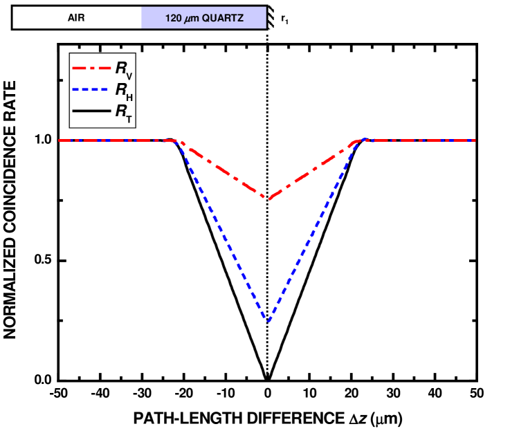
Figure 4: Simulation results for a single reflector buried beneath 120 $\mu$m of quartz with $n_{\rm e}=1.54661$, $n_{\rm o}=1.53773$, and $|r_{1}|^{2}=1$, using the scheme shown in Fig. 2. The optical axis of the quartz sample is aligned with the horizontal axis in the laboratory frame so that $\alpha_{1}=0$. The top two curves represent the normalized coincidence rate when the sample photon is mixed with a vertically polarized ($R_{\rm V}$, dash-dot curve) or a horizontally polarized ($R_{\rm H}$, dashed curve) reference photon. The solid curve represents the total coincidence rate ($R_{\rm T}$) from which the reflectance of the layer can be recovered.

Figure 4 displays the expected curves for a single reflector buried beneath 120 $\mu$m of quartz with $n_{\rm e}=1.54661$, $n_{\rm o}=1.53773$, and $|r_{1}|^{2}=1$, using the scheme shown in Fig. 2. For this simulation, we ignore the frequency dependence of $\delta$ [$\delta\equiv\delta(\omega_{0})$], assume that $\int d\Omega\,|\Phi(\Omega)|^{2}=1$, and select the fast axis of the quartz sample to be aligned with the horizontal axis in the laboratory frame so that $\alpha_{1}=0$. The SPDC spectrum is calculated explicitly via solutions to the phase-matching conditions using published Sellmeier equations for BBO. We are interested in the particular case of degenerate, collinear type-II phase matching. The top two curves represent the expected coincidence rate, normalized by $\Lambda_{0}$, when the sample photon is mixed with a vertically polarized ($R_{\rm V}$, dash-dot curve) or a horizontally polarized ($R_{\rm H}$, dashed curve) photon from the reference arm. The solid curve represents the re-normalized total coincidence rate [$R_{\rm T}=(R_{\rm V}+R_{\rm H}-\Lambda_{0})/\Lambda_{0}$] from which the reflectance of the layer can be recovered.

The material properties are revealed by the relative values at the center of the dip where $\tau=-4\beta^{\prime}z_{1}$. At this value of $\tau$, the path-length difference between the arms of the interferometer is zero and there is maximal quantum interference. If we neglect any frequency dependence in the birefringence, we can substitute Eq. (30) into Eq. (33) and write an expression for the coincidence rate at the center of the dip as

$$\Lambda(\tau=-4\beta^{\prime}z_{1})=|F_{1}|^{2}=|\cos\delta\,\cos 2\theta+\sin\delta\,\sin 2\theta\,e^{2{\rm i}\alpha_{1}}|^{2}.$$ (34)

In the particular case when we select the linear-rotator angle $2\theta$ to be either $0^{\circ}$ or $90^{\circ}$, corresponding to a polarization of the reference photon that is horizontal or vertical, respectively, we obtain

$$\Lambda_{\rm H} = \cos^{2}\delta$$

$$\Lambda_{\rm V} = \sin^{2}\delta.$$ (35)

It is possible to determine the value of $\delta$, or the birefringence $\Delta n$, by forming a ratio of these rates at $\Delta z=0$:

$$\delta=\tan^{-1}\left[{\frac{\Lambda_{\rm V}}{\Lambda_{\rm H}}}\right]^{\frac{1}{2}}=\omega_{0}\,\Delta n\,z_{1}/c.$$ (36)

We can neglect the frequency dependence of $\delta(\omega)=\omega\Delta n(\omega)\,z_{1}/c=\delta\beta(\omega)z_{1}$ when $\delta^{\prime}(\omega_{0})\,\Delta\Omega\ll 1$, where $\Delta\Omega$ is the bandwidth of the SPDC spectrum. In this limit, the width of the interference dip is larger than the delay between the signal and idler fields resulting from the birefringence of the layer. If the bandwidth of the SPDC spectrum is increased, the opposite limit can be realized, namely $\delta^{\prime}(\omega_{0})\,\Delta\Omega\gg 1$. In this case, the interference pattern comprises of three regions: the expected central dip at $\tau=-4\beta^{\prime}z_{1}$ provides the value of $\delta(\omega_{0})\equiv\delta$ as in Eq. (36); and two additional satellite interference patterns centered at $\tau=-[4\beta^{\prime}\pm 2\delta\beta^{\prime}]z_{1}$, where $\delta\beta^{\prime}$ is the coefficient of the first-order expansion of $\delta\beta$ in $\Omega$, and provide information about the group-velocity dispersion in the layer.

Since we choose the linear-rotator angles $2\theta$ to be either $0^{\circ}$ or $90^{\circ}$, any dependency of the coincidence rate according to the orientation angle $\alpha_{1}$ is lost. It is possible, however, to extract the value of $\alpha_{1}$ by using a technique that is analogous to null ellipsometry. In the reference arm, if we combine the linear-rotator used to rotate the linear input polarization state ${\bf e}_{\rm i}$ with a quarter-wave plate to transform the linear polarization into a general elliptical state, it is possible to exactly match any polarization state in the sample arm. This transformation is given by

$${\bf U}_{2}\,{\bf e}_{\rm i}=\frac{1}{\sqrt{2}}\begin{bmatrix}\cos 2\theta+{\rm i}\cos 2(\phi-\theta)\\ \sin 2\theta+{\rm i}\sin 2(\phi-\theta)\end{bmatrix},$$ (37)

where $\phi$ is the angle of the quarter-wave plate and $\theta$ is the angle of the linear rotator fast axes with respect to the horizontal axis. In the special case when $\phi=2\theta$, we revert to the case of a single linear rotator as in our previous example.

When the polarization in the reference arm is selected by this cascade of polarization elements, we can write Eq. (30) as

$$F_{1}(\omega)=\left\{\cos\delta(\omega)\,[\cos 2\theta-{\rm i}\cos 2(\phi-\theta)]+\sin\delta(\omega)\,[\sin 2\theta-{\rm i}\sin 2(\phi-\theta)]\,e^{2{\rm i}\alpha_{1}}\right\}.$$ (38)

If the values of $\phi$ and $\theta$ are adjusted so that the polarization state in the reference arm is exactly orthogonal to that in the sample arm, $|F_{1}|^{2}=0$ and the coincidence count rate will be maximized. The value for $\alpha$ can then be determined by solving the following conditions of orthonormality, namely, the real and/or imaginary parts of Eq. (38) must equal zero

$$\cos\delta\,\cos 2\theta+\sin\delta\,\sin 2\theta\,\cos 2\alpha_{1}-\sin\delta\,\sin 2(\phi-\theta)\,\sin 2\alpha_{1} = 0$$ (39)

$$-\cos\delta\,\cos 2(\phi-\theta)+\sin\delta\,\sin 2\theta\,\sin 2\alpha_{1}-\sin\delta\,\sin 2(\phi-\theta)\,\cos 2\alpha_{1} = 0.$$

If the value of $\delta$ is known, then only one of these equations is required.

IV.3 Two reflective layers

A sample with reflections from two surfaces separated by a birefringent material can be expressed as

$${\bf H}(\omega) = {\bf r}_{0}+{\bf S}_{1}\,{\bf r}_{1}\,{\tilde{\bf S}_{1}}$$ (40)

$$= {\bf r}_{0}+{\rm e}^{{\rm i}\,2\Delta_{1}}\,{\bf B}_{1}\,{\bf r}_{1}\,{\tilde{\bf B}_{1}}$$

where the subscripts $0$ and $1$ denote the first and second boundaries, respectively. In this case, the function in Eq. (16) becomes

$$F(\omega)={\rm i}\,r_{0}\,F_{0}+{\rm i}\,r_{1}\,{\rm e}^{{\rm i}\,2\Delta_{1}}\,F_{1},$$ (41)

where $F_{0}=\cos 2\theta$ and $F_{1}$ has been provided in Eq. (30).

For two reflectors separated by a birefringent medium, the constant and varying contributions from Eqs. (26) and (27) become

$$\Lambda_{0}=|r_{0}|^{2}\,\int d\Omega\,|\Phi(\Omega)|^{2}+|r_{1}|^{2}\,\int d\Omega\,|\Phi(\Omega)|^{2}+r_{0}^{\ast}\,r_{1}\,{\rm e}^{{\rm i}2\beta_{0}z_{1}}\,\int d\Omega\,|\Phi(\Omega)|^{2}{\bf u}^{\dagger}_{0}\,{\bf u}_{1}(\omega_{0}+\Omega)\,{\rm e}^{{\rm i}2(\beta^{\prime}\Omega+\beta^{\prime\prime}\Omega^{2})z_{1}}+cc.$$ (42)

and

$$\Lambda({\tau})=|r_{0}|^{2}\,g^{(0)}(\tau)+|r_{1}|^{2}\,g^{(1)}(\tau-4\beta^{\prime}z_{1})+r_{0}^{\ast}\,r_{1}\,g^{(01)}_{\rm d}(\tau-2\beta^{\prime}z_{1})\,{\rm e}^{{\rm i}2\beta_{0}z_{1}}+cc.,$$ (43)

respectively, where the subscript ${\rm d}$ denotes a contribution that is subject to even-order dispersion and $cc$ indicates the complex conjugate, with

$$g^{(m)}(\tau)=\int d\Omega\,|\Phi(\Omega)|^{2}\,F_{m}(\omega_{0}+\Omega)\,F_{m}^{\ast}(\omega_{0}-\Omega)\,{\rm e}^{-{\rm i}\Omega\tau}$$

and

$$g_{\rm d}^{(mn)}(\tau)=\int d\Omega\,|\Phi(\Omega)|^{2}\,F_{m}(\omega_{0}+\Omega)\,F_{n}^{\ast}(\omega_{0}-\Omega)\,{\rm e}^{{\rm i}2z_{1}\beta^{\prime\prime}\Omega^{2}}\,{\rm e}^{-{\rm i}\Omega\tau}.$$

The first two terms in Eq. (42) are contributions to the constant coincidence rate arising from each of the two interfaces in the material. The third term introduces a contribution only when these interfaces have a separation that is less than the coherence length of the signal photon. The first two terms in Eq. (43) represent dips arising from reflections from the first and second surfaces. The third term, which appears midway between these dips, arises from the interference between probability amplitudes associated with each of these reflections.

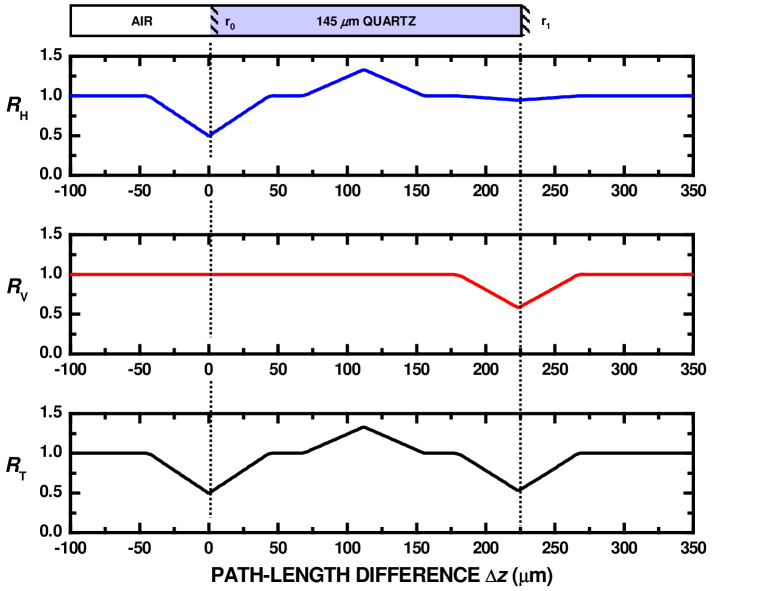
Figure 5: Simulation results for a 145-$\mu$m quartz sample with reflections from each interface using the scheme shown in Fig. 2. For this calculation, $n_{\rm e}=1.54661$, $n_{\rm o}=1.53773$, and $|r_{0}|^{2}=|r_{1}|^{2}$. The optical axis of the quartz is aligned with the horizontal axis in the laboratory frame so that $\alpha_{1}=0$. The top two plots represent the normalized coincidence rate when the sample photon is mixed with a horizontally polarized ($R_{\rm H}$) or a vertically polarized ($R_{\rm V}$) reference photon. The bottom trace represents the total coincidence rate ($R_{\rm T}$) from which the relative reflectance of each interface can be recovered. The separation of the dips is given by the optical path length of the quartz ${\bar{n}}L\simeq 224~{}\mu$m.

Figure 5 provides numerical results for a 145-$\mu$m quartz sample with reflections from each of the two surfaces. For this calculation, again $n_{\rm e}=1.54661$, $n_{\rm o}=1.53773$, we ignore the frequency dependence of $\delta$, and the fast axis of the quartz plate is aligned with the horizontal axis in the laboratory frame so that $\alpha_{1}=0$. The magnitude of the reflectance from each surface is assumed to be the same so that $|r_{0}|^{2}=|r_{1}|^{2}$. The SPDC spectrum is calculated explicitly via solutions to the phase-matching conditions using published Sellmeier equations for BBO. We are interested in the particular case of degenerate, collinear type-II phase matching. The top two plots represent the expected rate of coincidence when the sample photon is mixed with a horizontally polarized ($R_{\rm H}$) or a vertically polarized ($R_{\rm V}$) reference photon. The bottom trace represents the re-normalized total coincidence rate [$R_{\rm T}=(R_{\rm V}+R_{\rm H}-\Lambda_{0})/\Lambda_{0}$] from which the relative reflectance and positions of each interface can be determined.

In the $R_{\rm V}$ curve (middle trace), there is no dip at the first interface since the polarization mode reflected from this interface is solely horizontal. The polarization state is altered via propagation through the birefringent material and contains both vertically and horizontally polarized photons at reflection from the second interface. The peak between the two interfaces in $R_{\rm H}$ (top trace) and $R_{\rm T}$ (bottom trace) is result of interference between each layer. This peak (which can alternatively become a dip depending on the phase accumulated between the layers) is susceptible to dispersion in the sample, unlike the dips that correspond to sample layers. Thus the dispersion properties of the material can be extracted from this feature.

In summary, we ascertain that three experiments are required to completely determine the sample properties. We first select the reference arm polarization to be horizontal (H) and measure the quantum interferogram $R_{\rm H}$ by recording the coincidence rate of photons arriving at the two detectors as the path-length delay $c\tau$ is scanned. The reference arm polarization is then rotated into the orthogonal vertical (V) polarization and a second measurement is made to measure the quantum interferogram $R_{\rm V}$. The third measurement is made by selecting a value of $c\tau$ that coincides with the position of a layer. The angles of the polarization elements in the reference arm are then adjusted to maximize the coincidence rate.

The sample properties are found as follows: by forming a ratio of $\Lambda_{\rm V}$ and $\Lambda_{\rm H}$ at a value of $c\tau$ that coincides with the position of a layer, we can determine the value of the birefringence contained in the parameter $\delta$; using the angles from the polarization elements in the reference arm, $\alpha$ can be found from solving the equations for orthonormality. This technique is similar to nulling techniques in ellipsometry; and the total quantum interferogram $R_{\rm T}$ can be computed from the sum of $R_{\rm H}$ and $R_{\rm V}$, then readjusted for the dc offset given by the constant term $\Lambda_{0}$, i.e. $R_{\rm T}=(R_{\rm V}+R_{\rm H}-\Lambda_{0})/\Lambda_{0}$. The $R_{\rm T}$ curve provides the path-length delay between the interfaces as well as the ratio of the relative reflectance from each layer.

V CONCLUSION

We have set forth a new polarization-sensitive QOCT (PS-QOCT) scheme and provide a general Jones matrix theory for analyzing its operation. PS-QOCT provides a means for determining information about the optical path length between isotropic reflectors, the relative magnitude of the reflectance from each interface, the birefringence of the material between the interfaces, and the orientation of the optical axis $\alpha$ of the sample. Inasmuch as PS-QOCT is immune to sample dispersion, measurements are permitted at depths greater than those accessible via ordinary optical coherence tomography.