TU- 709

Complete Resolution
of the Quantum Zeno Paradox
for Outside Observers

M.Hotta^∗ and M.Morikawa^†
∗ Department of Physics, Faculty of Science, Tohoku University,
Sendai 980-8578,Japan
hotta@tuhep.phys.tohoku.ac.jp

^† Physics Department, Ochanomizu University,
Tokyo, 112-8610, Japan
hiro@phys.ocha.ac.jp

The quantum Zeno paradox is fully resolved for purely indirect and incomplete measurements performed by the detectors outside the system. If the outside detectors are prepared to observe propagating signals of a decay event of an excited state in the core region, the survival probability of the state is not changed at all by the outside measurements, as long as the wavefunction of the signals does not have reflectional-wave contributions going back to the core by the outside detectors. The proof is independendent of the decay law of the survival probabilities. Just watching frequently from outside (observation) cannot be regarded as a measurement which yields the quantum Zeno effect.

1 Introduction

The quantum Zeno (QZ) paradox [1] has been tempting a lot of physicists to make the complete and elegant resolution for long years. The quantum theory predicts, as will be mentioned in the next section, that quantum processes are frozen by their continuous measurements.  However the predicted freezing of the processes apparently contradicts macroscopic reality.

To express the QZ paradox microscopically, a phrase is available; an unstable particle does not decay under the frequent monitoring. For example, the proton was expected to decay within the lifetime of order $10^{30}$ years and sensitive experiments for the proton decay have been performed. Unfortunately, no signal has been found so far and the elementary particle physicists have changed the “wrong” Lagrangians of their models for the decay so as to prolong the lifetime.  From the view point of the QZ effect, there is another possible solution to explain why the proton decay has not actually been observed[2]; sensitive devices in the experiment have monitored the decay process too frequently and therefore have frozen the decay process.

Amazingly, the QZ paradox is also applied to the well known Schrödinger’s cat system. Suppose that an excited state of an atom decays and emits photons, and that the detection of the photons by a measurement device triggers the death of his cat. Then it is possible to propose an interesting paradox; the cat’s lifetime is prolonged by the continuous observation of the cat. We can assume, once the excited state decays, that the time interval from the photon emission to the cat’s death is instantaneous. Then, each survival result of the cat by the observation directly implies that the excited state of the atom has not yet decayed. Thus, the observation of the cat is an indirect measurement of the atom itself. According to the QZ effect, the continuous measurement of the atom should prolong the decay of the excited state. Consequently, the lifetime of the cat should also be prolonged.

Nowadays, the QZ paradox is a quite exciting issue for not only theorists but also experimentalists. In fact, several experiments for the QZ effect have been already performed and showed the evidence that the frequent measurements actually make the quantum processes slower in some systems [3].

Although such successful experiments have been achieved, we cannot say that the essential part of the QZ paradox has fully been solved. The experiments were performed only by use of direct measurements of unstable systems. In order to observe the measurement effect, the system was coupled directly and strongly with other ancilla states, and(or) was immersed in the external strong pulsed waves. Clearly, such operations induce additional interaction terms in the system Hamiltonian and drastically modify the dynamics in the closed regions. Thus, strictly speaking, there is no surprise even if the strong direct measurements yield prominent phenomena like freezing of the system evolution. In order to resolve the QZ paradox completely, the analysis of purely indirect measurements of the system is inevitable . The QZ paradox becomes indeed serious, for instance, when the signals emitted by an unstable system at the decay time propagate away from the system and are measured by outside devices. However actually, such experiments have not been realized so far. Therefore we do not have any experimental evidence that the QZ paradox occurs under the continuous and purely indirect measurements. Note that the above examples of the QZ paradox are all based on the purely indirect measurements.  In the proton decay example, photo-multipliers on the wall of water storage tank observe Cherenkov beams emitted by electric showers which are formed by the proton decay in the water. In the Schrödinger’s cat example, not the unstable atom but the cat is observed. Therefore, it is of great importance to check whether the quantum theory really generates the QZ paradox in the purely indirect measurements or not.

In general, the emitted signals (photons and so on), which imply the decay of the unstable state, reach the wave zone eventually after the launch from the core system. We defined naturally in the previous paper [4] the wave-zone states and wave-zone subspace for the signals in the Hilbert space. Then, it was shown that no QZ paradox appears in the indirect and ideal measurements of the wave-zone states. In this paper, we critically analyze the QZ paradox again, taking account of finite errors of the general indirect measurements. Using the definition of the wave-zone states, a no-go theorem of the QZ paradox under general indirect measurements with finite errors is proven; no indirect measurements by use of the signals affect the survival probability of the unstable core state at all when the measurements of the signals are performed in the wave-zone states, as long as the wavefunction of the signals do not have any reflectional contributions back to the core system by the detectors. Thus we argue that the no-go theorem fully resolves the QZ paradox under purely indirect measurements. For instance, the quantum theory indeed predicts that the unstable particle decays even if the outside apparatus monitors continuously, and that the lifetime of the Schrödingers cat is not prolonged by the cat observations.

The outline of this paper is as follows. In the next section 2, we review briefly the standard QZ argument. In the section 3, we specify in the simplest form the general feature of the purely indirect the QZ experiments with finite errors. Under some conditions, we prove the impossibility of the QZ effect in the purely indirect distant measurements. Based on this argument, in section 4, we study a simple model which demonstrates this impossibility of the QZ effect. In the last section, we summarize the results.

2 The Quantum Zeno Paradox under the Continuous and Direct Measurements

Let us first explain the quantum Zeno (QZ) paradox in the standard way. Consider a quantum system with unitary evolution. The Hamiltonian is given by $H$. Suppose that the Hamiltonian $H$ is the sum of the free evolution term $H_{o}$ and the interaction term $H_{int}$, which generates dynamical transitions from an eigenstate state $|e\rangle$ of $H_{o}$ to the other state or decay of the state $|e\rangle$;

$$H=H_{o}+H_{int},$$ (1)

where $H_{o}|e\rangle=E_{o}|e\rangle$. Then let us focus on the survival probability $s(t)$ of the state $|e\rangle$ ;

$$s(t)=|\langle e(0)|e(t)\rangle|^{2},$$ (2)

where $|e(t)\rangle$ is the time evolved state from the initial state $|e(0)\rangle=|e\rangle$ at time $t$. According to the time reversal symmetry, $s(t)$ behaves at short times like

$$s(\Delta t)\sim 1-\alpha\Delta t^{2},$$ (3)

where $\alpha$ is a positive constant. Therefore, at time $t=N\Delta t$ after N successive direct measurements of the state, the survival probability of the state is evaluated as

$$s_{N}(t)\sim\left(1-\alpha(\Delta t)^{2}\right)^{\frac{t}{\Delta t}}\sim e^{-\alpha t\Delta t}.$$ (4)

Consequently in the continuous measurement of the state ( in the limit $N\rightarrow\infty$, $\Delta t\rightarrow 0$ with $t$ fixed) one obtains

$$\lim_{N\rightarrow\infty}s_{N}(t)=1,$$ (5)

thus the time evolution of the state $|e\rangle$ freezes. This explicitly shows the appearance of the QZ paradox.

It is known that direct measurements with finite errors can also partially freeze the time evolution of the system[5]. Let us consider ancilla system which represents the measurement apparatus. Suppose that a direct interaction $gH_{m}$ is turned on between the system and the measurement apparatus, where $g$ is a real coupling constant and $H_{m}$ is a Hermitian operator. For simplicity, we assume that the initial state $|e\rangle$ is the eigenstate with zero eigenvalue of $H_{m}$;

$$H_{m}|e\rangle=0.$$ (6)

The term “direct” means here that the measurement Hamiltonian does not commute with the interaction Hamiltonian $H_{i}$; $[gH_{m},\ H_{i}]\neq 0$. By adding $gH_{m}$ to $H$, the total Hamiltonian now reads

$$H_{tot}=H+gH_{m}=H_{o}+H_{i}+gH_{m}.$$ (7)

The time evolution under the measurement is generated by this $H_{tot}$. Here finiteness of the coupling $g$ implies incompleteness of the measurement, that is, the non-ideal measurement with finite errors. Let us suppose that the coupling $g$ is finite, but large enough and that the eigensubspace with the zero eigenvalue of the Harmitian operator $H_{m}$ is non-degenerate, that is, a one-dimensional space.  Then, it is shown that the survival probability $s_{g}(t)$ of the state $|e\rangle$ becomes larger than the value without measurement (the case of $g=0$). This type of disturbance on the evolution is generally called QZ effect as well.

This general QZ effect under observations with finite errors has a distinguished property for the measurement of the exponentially decaying systems.  The ideal measurements, no matter how frequent,  do not change at all the exponential decay law, $s(t)\propto e^{-\Gamma t}$, which appears in the intermediate time scales of many systems. The following evaluation shows this fact:

$$\lim_{N\rightarrow\infty}s_{N}(t)\propto\lim_{N\rightarrow\infty}\left(1-\Gamma\Delta t\right)^{\frac{t}{\Delta t}}=e^{-\Gamma t}.$$ (8)

On the other hand, surprisingly, it is proven [6] that incomplete measurements can change the exponential decay law and show the QZ or anti-QZ effect. This fact makes studies of the general measurements with finite errors more important.

In the next section we study purely indirect measurements with finite errors and discuss the possibility of the QZ paradox in this case.

3 No-Go Theorem

In general, the total quantum system including the measurement apparatus may actually be very complicated.  However a subspace $\mathcal{H}_{Z}$ which is relevant to consider the QZ effect would be almost closed in dynamics. We would like to concentrate on this subspace $\mathcal{H}_{Z}$.  Let $\{|e\rangle,\{|n\rangle\}_{n=1,2,...}\}$ denote the complete orthonormal basis vectors in $\mathcal{H}_{Z}$.

Let us denote $|e(t)\rangle$ as the time evolved state at time $t$ from the initial state $|e(0)\rangle=|e\rangle$.  Since the evolution of the state vector is closed in this space,

$$|e(t)\rangle=A(t)|e\rangle+\sum_{n}a_{n}(t)|n\rangle,$$ (9)

the survival probability of the state $|e\rangle$, $s(t):=|\langle e(0)|e(t)\rangle|^{2}=|A(t)|^{2}$, can be obtained without direct measurements of the state $|e\rangle$. Actually, the measurements of the states $|n\rangle$ provide us the probability $s(t)$ through the unitary relation:

$$s(t)=1-\sum_{n}|a_{n}(t)|^{2}.$$ (10)

This operation is called as indirect measurement of $s(t)$.  For the specification of the indirect measurement, we should have to add one important property.  When we measure the states $|n\rangle$, we must couple the states with some measurement devices. This measurement interaction must commute with the original interaction in the system.  Otherwise, the measurement directly modifies the system dynamics and the measurement cannot be regarded as purely indirect.

In order to define generally and rigorously the purely indirect measurements, let us define the core-zone and wave-zone states in the space $\mathcal{H}_{Z}$, in the same manner as

in the paper [4].

Definition
We define the maximal subspace $\mathcal{H}_{W}$ ($\subset$ $\mathcal{H}_{Z}$), which is invariant under the advanced time evolution $U_{+}(t)=e^{-\frac{i}{\hbar}tH}$: $U_{+}(t)\mathcal{H}_{W}$ =$\mathcal{H}_{W}$  for all $t\geq 0$, where $H$ is the Hamiltonian of the system.  In other words,

$$If\quad|W\rangle\in\mathcal{H}_{W},\quad U_{+}(t)|W\rangle\in\mathcal{H}_{W}\quad\ for\quad all\quad t\geq 0.$$ (11)

This simply says that any vector $|W\rangle$ in $\mathcal{H}_{W}$ evolves within $\mathcal{H}_{W}$ in the future.  Then the space $\mathcal{H}_{Z}$ can be decomposed into mutually complementary subspaces $\mathcal{H}_{C}$ and $\mathcal{H}_{W}$:

$$\mathcal{H}_{Z}=\mathcal{H}_{C}\oplus\mathcal{H}_{W}.$$ (12)

We call $\mathcal{H}_{C}$ the core subspace and $\mathcal{H}_{W}$ the wave-zone subspace.  For a practically meaningful systems, we assume both are non-empty subspaces:

$$\mathcal{H}_{C}\neq\o,\ and\quad\mathcal{H}_{W}\neq\o.$$ (13)

We call $|C\rangle(\in\mathcal{H}_{C})$ a core-zone state and $|W\rangle(\in\mathcal{H}_{W})$ a wave-zone state.

To understand the physical meaning of the above definition of the wave-zone state, let us consider that an unstable excitation in the core region of the system decays and simultaneously emits photons, which propagate away from the core and are measured by the outside devices. The wave-zone states defined above faithfully describe the outside photon behaviors; the emitted photons from the core eventually reach the wave zone, that is, the photons begin to propagate freely in the space and never come back to the emission core. Hence, advanced time evolution of the photon states in the wave zone would never affect the transition amplitudes in the core-zone states.

Clearly, the emergence of nontrivial subspace $\mathcal{H}_{W}$ is allowed only when $\mathcal{H}_{W}$ is an open system. Also note that the invariance $U_{+}(t)\mathcal{H}_{W}$ =$\mathcal{H}_{W}$  itself cannot uniquely determine the wave-zone subspace $\mathcal{H}_{W}$.  We are interested in the largest $\mathcal{H}_{W}$ and the smallest $\mathcal{H}_{C}$.  The boundary between $\mathcal{H}_{W}$ and $\mathcal{H}_{C}$ only admits a one-way flow of states in the direction of future.

Now we concentrate on the indirect measurements in the wave-zone subspace, in which the wavefunction of the observed signals does not have reflectional-wave contributions going back to the emission core after the measurements. If a reflectional wave which goes back to the core exists and produces the inverse decay process at the core, then this measurement cannot be regarded as indirect. This is because the returning wave, after the collision to the core, may excite the unstable state again. Therefore the returning wave behaves just as an extra incident wave to the core system. Hence, the reflectional effect, if it exists, ought to be called “semi-direct” and is out of our interest.

The above definition of the wave-zone subspace $\mathcal{H}_{W}$ can also be possible for the extended system which includes the measurement devices. The non-existence of the reflectional wave induced by the measurement is characterized by

$$P_{W}H_{m}P_{W} = H_{m},$$ (14)

$$P_{C}H_{i}P_{C} = H_{i}.$$ (15)

These equations leads $[H_{m},H_{i}]=0.$  In this paper, general purely indirect measurements in the wave-zone subspace $\mathcal{H}_{W}$ are defined by this relation (14).

Let us introduce the projection operator $P_{C}$ onto $\mathcal{H}_{C}$ as

$$P_{C}=|e\rangle\langle e|+\sum_{c}|c\rangle\langle c|,$$ (16)

where $\{|e\rangle,|c\rangle\}$ is the complete orthonormal basis of $\mathcal{H}_{C}$. The projection operator onto $\mathcal{H}_{W}$ is

$$P_{W}=\sum_{w}|w\rangle\langle w|,$$ (17)

where $\{|w\rangle\}$ is the orthonormal complete basis of $\mathcal{H}_{W}$. The time evolution of the core-zone state $|e\rangle(\in\mathcal{H}_{C})$ now reads the following closed form;

$$|e(t)\rangle = U_{g+}(t)|e\rangle$$ (18)

$$= A(t)|e\rangle+\sum_{c}a_{c}(t)|c\rangle+\sum_{w}a_{w}(t)|w\rangle,$$

where the operator $U_{g+}$ is the advanced time evolution operator including the measurement effect which is defined by

$$U_{g+}(t\geq 0):=\exp\left[-i\frac{t}{\hbar}\left(H+gH_{m}\right)\right]$$ (19)

and the normalization condition, $|A(t)|^{2}+\sum_{c}|a_{c}(t)|^{2}+\sum_{w}|a_{w}(t)|^{2}=1$, is satisfied.

The above wave-zone property eqn.(11) can be concisely described by using the projection operators just introduced.  The eqn.(11) means “wave-zone states evolve within $\mathcal{H}_{W}$ in the future”:$[P_{W},U_{+}]P_{W}=0.$ Since $P_{C}+P_{W}=\mathbf{1}_{Z},$ this leads $[P_{C},U_{+}]P_{W}=0,$ which is equivalent to

$$P_{C}U_{+}(t)P_{W}=0.$$ (20)

Now let us define the survival probability of the genuine core-zone state $|e\rangle$ under the purely indirect measurement as

$$s_{g}(t):=\left|\langle e|U_{g+}(t)|e\rangle\right|^{2}.$$ (21)

Then we prove a no-go theorem for the QZ paradox under the purely indirect measurement as follows.

Theorem

We prepare a system with a measurement apparatus, and suppose the total state space admitts the decomposition into a core-zone subspace $\mathcal{H}_{C}$ and a wave-zone subspace $\mathcal{H}_{W}$.  For this system, we operate a purely indirect measurement with the Hamiltonian given by $gH_{m}$, where $g$ is a real coupling constant and $H_{m}$ is a Hermitian operator satisfying $P_{W}H_{m}P_{W}=H_{m}$. Then, the survival probability $s_{g}(t)$ of a core-zone state $|e\rangle(\in\mathcal{H}_{C})$ does not depend on the measurement coupling constant $g$;

$$s_{g}(t):=\left|\langle e|U_{g+}(t)|e\rangle\right|^{2}=\left|\langle e|U_{+}(t)|e\rangle\right|^{2}=s_{0}(t).$$ (22)

This theorem implies that the measurement never affect the time evolution of the state $|e(t)\rangle$ even if the measurement interaction becomes extremely strong, $g\rightarrow\infty$. Consequently, the QZ paradox does not take place under the purely indirect measurement.

The proof of the theorem is given as follows. Let us define a unitary operator $V_{g}(t)$ as

$$V_{g}(t)=U_{g+}(t)U_{+}^{\dagger}(t),$$ (23)

where $V_{g}(0)=\mathbf{1}$ is satisfied. Then, this operator obeys the following equation;

$$i\hbar\partial_{t}V_{g}(t)=gV_{g}(t)U_{+}(t)H_{m}U_{+}^{\dagger}(t).$$ (24)

By applying $P_{C}$ from the left in this equation and using the relation $H_{m}=P_{W}H_{m}P_{W}$, we obtain a differential equation of first order with respect to time $t$;

$$\partial_{t}[P_{C}V_{g}(t)]=-i\frac{g}{\hbar}[P_{C}V_{g}(t)][U_{+}(t)P_{W}H_{m}P_{W}U_{+}^{\dagger}(t)].$$ (25)

Note that the initial condition for the operator $P_{C}V_{g}(t)$ is given by $P_{C}V_{g}(0)=P_{C}$. Under this initial condition, eqn(25) is solved at time $t\geq 0$ as

$$P_{C}V_{g}(t\geq 0)=P_{C}.$$ (26)

Using the wave-zone property in the form eqn.(20), this is easily checked by substituting eqn(26) into eqn(25). Rewriting eqn(26) yields the crucial relation;

$$P_{C}U_{g+}(t)=P_{C}U_{+}(t).$$ (27)

Now, using eqn(27) and $\langle e|=\langle e|P_{C}$, we can manipulate as follows.

$$s_{g}(t)=\left|\langle e|P_{C}U_{g+}(t)|e\rangle\right|^{2}=\left|\langle e|P_{C}U_{+}(t)|e\rangle\right|^{2}=s_{0}(t).$$ (28)

Thus, the theorem is proved. Extension of the proof to the cases with many coupling constants $g_{i}$ or coupling functions $g_{i}(x)$ is possible in the similar way.

In the next section, we give a simple example to which the theorem can be applicable rigorously.

4 A Model

In this section, we study a simple example which possesses a wave-zone subspace and the no-go theorem for the QZ paradox is applicable rigorously.

The model is the same as that introduced in the previous paper [4]. In what follows let us explain the model in detail. We set a two-level atom system of size $d$ in one-dimensional space, in which $x$ denotes its spatial coordinate, on the region $[-d/2,d/2]$. (Fig. 1 upper diagram)

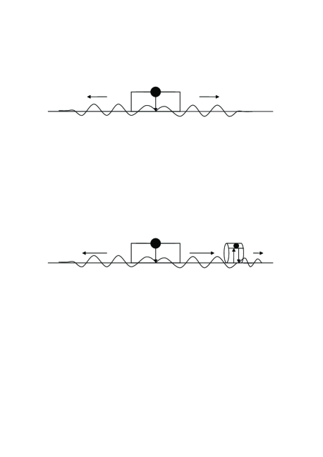
Figure 1: Schematic diagrams of the model.
[Upper diagram] A two-level atom system of size $d$ in one-dimensional $x$-coordinate space. The system is located at $[-d/2,d/2]$, and emits spinor pair when it decays.
[Lower diagram] The system is coupled to a detector, which is located at $[x_{-},x_{+}]$ on the right hand side of the atom. The detector measures the spinor field.

To express the upper and lower energy level states, we introduce a fermionic pair of annihilation and creation operators $a$ and $a^{\dagger}$:

$$\{a,\ a^{\dagger}\}=1,$$ (29)

$$\{a^{\dagger},\ a^{\dagger}\}=\{a,\ a\}=0.$$ (30)

We also introduce a massless spinor field

$$\Phi(x)=(\Phi_{R}(x),\Phi_{L}(x))^{T}$$ (31)

and quantize it in the fermionic way:

$$\{\Phi_{h}(x),\ \Phi_{h^{\prime}}^{\dagger}(x^{\prime})\}=\delta_{hh^{\prime}}\delta(x-x^{\prime}),$$ (32)

$$\{\Phi_{h}^{\dagger}(x),\ \Phi_{h^{\prime}}^{\dagger}(x^{\prime})\}=\{\Phi_{h}(x),\ \Phi_{h^{\prime}}(x^{\prime})\}=0,$$ (33)

where $h(=R,L)$ is the helicity of the field excitations. As in the Coleman-Hepp model [7] the vacuum state $|vac\rangle$ is introduced using the annihilation operator as

$$a|vac\rangle=0,$$ (34)

$$\Phi_{h}(x)|vac\rangle=0.$$ (35)

Then the excited state of the two-level atom is defined by

$$|e\rangle=a^{\dagger}|vac\rangle.$$ (36)

For the spinor field, we concentrate on the two particle states in which only one R-helicity and one L-helicity particles exist. The state in which a R-helicity particle stays at the position $x=x_{R}$ and a L-helicity particle at $x=x_{L}$ is denoted by

$$|x_{R},x_{L}\rangle=\Phi_{R}^{\dagger}(x_{R})\Phi_{L}^{\dagger}(x_{L})|vac\rangle.$$ (37)

Now let us write the Hamiltonian of the total system; it is composed of three terms:

$$H=H_{atom}+H_{\Phi}+H_{int}.$$ (38)

The first term $H_{atom}$ is the Hamiltonian of free motion of the two-level atom and is given by

$$H_{atom}=\hbar\omega a^{\dagger}a.$$ (39)

The energy of the excited state is set to be $\hbar\omega$. The second term $H_{\Phi}$ is the free Hamiltonian of the massless spinor field and is defined by

$$H_{\Phi} = -i\hbar c\int_{-\infty}^{\infty}\Phi^{\dagger}\sigma_{3}\partial_{x}\Phi dx$$ (40)

$$= -i\hbar c\int_{-\infty}^{\infty}\left[\Phi_{R}^{\dagger}\partial_{x}\Phi_{R}-\Phi_{L}^{\dagger}\partial_{x}\Phi_{L}\right]dx,$$

where $\sigma_{3}$ is the third component of the Pauli matrix. If no interaction term is added, the field Hamiltonian yields right-moving particles for $h=R$ and left-moving particles for $h=L$ with the light velocity. The third term $H_{int}$ in eqn.(38) expresses the interaction between the two-level atom and the spinor field and is given by

$$H_{int} = \hbar\int_{-d/2}^{d/2}dx\int_{-d/2}^{d/2}dx^{\prime}$$ (41)

$$\times\left[g(x,x^{\prime})\Phi_{R}^{\dagger}(x)\Phi_{L}^{\dagger}(x^{\prime})a+g(x,x^{\prime})^{\ast}a^{\dagger}\Phi_{L}(x^{\prime})\Phi_{R}(x)\right].$$

The interaction is supposed to take place only in the atom region $(-d/2,d/2)$, i.e. the support of $g(x,x^{\prime})$ is $(-d/2,d/2)$, and the excited state of the atom decays into two particle states with different helicities. Note that even after adding the interaction term in eqn.(41), $|vac\rangle$ is still stable.

In this model the subspace, whose complete basis is given by $\{|e\rangle,|x_{R},x_{L}\rangle\}$ with $x_{R}\geq-d/2$ and $x_{L}\leq d/2$, is identified as $\mathcal{H}_{Z}$, because the evolution in this space is closed:

$$|\Psi(t)\rangle=C(t)|e\rangle+\int_{-d/2}^{\infty}dx_{R}\int_{-\infty}^{d/2}dx_{L}F(x_{R},x_{L};t)|x_{R},x_{L}\rangle$$ (42)

for an arbitrary vector $|\Psi\rangle(\in\mathcal{H}_{Z})$. From the Schröddinger equation, the amplitudes obey the following equations:

$$i\partial_{t}C=\omega C(t)+\int_{-d/2}^{d/2}dx_{R}\int_{-d/2}^{d/2}dx_{L}g(x_{R},x_{L})^{\ast}F(x_{R},x_{L};t),$$ (43)

$$(\partial_{t}+c\partial_{x_{R}}-c\partial_{x_{L}})F(x_{R},x_{L};t)=-ig(x_{R},x_{L})C(t).$$ (44)

This eqn.(44) can be integrated to yield

$$F(x_{R},x_{L};t) = F_{o}(x_{R}-ct,x_{L}+ct)$$ (45)

$$-i\int_{0}^{t}g(x_{R}-ct+c\tau,x_{L}+ct-c\tau)C(\tau)d\tau,$$

where $F_{o}(x_{R},x_{L})$ is the initial amplitude of $F$ at $t=0$.

When $x_{R}>d/2$ or $x_{L}<-d/2$, by taking the initial condition as

$$C(0)=0,$$ (46)

$$F_{o}(x_{R},x_{L})=\delta(x_{R}-x_{R}^{\prime})\delta(x_{L}-x_{L}^{\prime}),$$ (47)

the following relation arises from eqn.(43) and eqn.(45);

$$U_{+}(t)|x_{R},x_{L}\rangle=|x_{R}+ct,x_{L}-ct\rangle.$$ (48)

This means that the right- and left-moving particles propagate freely after leaving the interaction region. It is worth stressing that even if only one of the two conditions $x_{R}>d/2$ or $x_{L}<-d/2$ holds, the evolution in eqn (48) is still realized. This is because the interaction is activated only when the both particles simultaneously stay in $(-d/2,d/2)$.

From the above result, we can introduce in $\mathcal{H}_{Z}$ a wave-zone subspace $\mathcal{H}_{W}$ orthogonal to the excited state $|e\rangle$, which is defined using the projection operator onto the subspace $P_{W}$:

$$P_{W}=P_{R}+P_{L}+P_{RL},$$ (49)

$$P_{R} = \int_{d/2}^{\infty}dx_{R}\int_{-d/2}^{d/2}dx_{L}|x_{R},x_{L}\rangle\langle x_{R},x_{L}|,$$ (50)

$$P_{L} = \int_{-d/2}^{d/2}dx_{R}\int_{-\infty}^{-d/2}dx_{L}|x_{R},x_{L}\rangle\langle x_{R},x_{L}|,$$ (51)

$$P_{RL} = \int_{d/2}^{\infty}dx_{R}\int_{-\infty}^{-d/2}dx_{L}|x_{R},x_{L}\rangle\langle x_{R},x_{L}|.$$ (52)

Then the core-zone subspace $\mathcal{H}_{C}$ is defined, using this projection operator, as

$$P_{C}:={}1_{Z}-P_{W}=|e\rangle\langle e|+\int_{-d/2}^{d/2}dx_{R}\int_{-d/2}^{d/2}dx_{L}|x_{R},x_{L}\rangle\langle x_{R},x_{L}|.$$ (53)

By construction,

$$P_{C}|e\rangle=|e\rangle.$$ (54)

Now the states are complete in $\mathcal{H}_{Z}$ as seen in eqn (42), and the wave-zone property in eqn(11) holds due to the relation eqn.(48), we are ready to apply the theorem in the previous section. In what follows, we discuss purely indirect measurements with finite errors in the wave-zone subspace.

Let us consider that a measurement apparatus is set at the location $[x_{-},x_{+}]$ on the right hand side of the atom: $x_{+}>x_{-}>d/2$(Fig.1 lower diagram); the apparatus measures the $\Phi$ field with the following interaction:

$$H_{m1} = \hbar\int_{-\infty}^{\infty}\Omega(k)b^{\dagger}(k)b(k)dk$$ (55)

$$+\hbar\int_{x_{-}}^{x_{+}}dx\int_{-\infty}^{\infty}dk\lambda_{R}(x,k)\left(b^{\dagger}(k)\Phi_{R}(x)+\Phi_{R}^{\dagger}(x)b(k)\right),$$

where $b(k)$ ($b^{\dagger}(k)$) is the annihilation (creation) operator of the detector excitations:

$$[b(k),\ b^{\dagger}(k^{\prime})]=\delta(k-k^{\prime}),$$

and $\Omega(k)$ and $\lambda_{R}(x)$ are real coupling functions.  The function $\lambda_{R}(x)$ has its support on $[x_{-},x_{+}]$ and controls the incompleteness of the detector.

Here let us extend the projection operator $P_{W}$ to

$$P_{W1}=P_{R}+P_{L}+P_{RL}+P_{ML},$$ (56)

where

$$P_{ML}:=\int_{-\infty}^{d/2}dx_{L}\int_{-\infty}^{\infty}dk|k;x_{L}\rangle\langle k;x_{L}|,$$ (57)

and

$$|k;x_{L}\rangle:=b^{\dagger}(k)\Phi^{\dagger}(x_{L})|vac\rangle.$$ (58)

Then, it is checked that the subspace defined by $P_{W1}$ is really a wave-zone subspace $P_{C}U_{+}(t)P_{W1}=0,$ complementary to $\mathcal{H}_{C}$; $P_{C}+P_{W1}=$ ${}1_{Z}$. Further it is trivial by construction that

$$P_{W1}H_{m1}P_{W1}=H_{m1}.$$ (59)

Consequently we can apply the no-go theorem, and conclude that no QZ paradox appears in this purely indirect measurement with finite errors.

It may be instructive to prove again the theorem for this model, explicitly using the Schrödinger equation. The time evolution in this case can be expressed in a closed form as

$$|\Psi(t)\rangle = C(t)|e\rangle+\int_{-d/2}^{\infty}dx_{R}\int_{-\infty}^{d/2}dx_{L}F(x_{R},x_{L};t)|x_{R},x_{L}\rangle$$ (60)

$$+\int_{-\infty}^{d/2}dx_{L}\int_{-\infty}^{\infty}dkD_{k}(x_{L};t)|k;x_{L}\rangle.$$

The equations of motion read

$$i\partial_{t}C(t)=\omega C(t)+\int_{-d/2}^{d/2}dx_{R}\int_{-d/2}^{d/2}dx_{L}g(x_{R},x_{L})^{\ast}F(x_{R},x_{L};t),$$

$$(\partial_{t}+c\partial_{x_{R}}-c\partial_{x_{L}})F(x_{R},x_{L};t)$$ (61)

$$= -ig(x_{R},x_{L})C(t)-i\int_{-\infty}^{\infty}dk\lambda_{R}(x_{R},k)D_{k}(x_{L};t),$$

$$i\partial_{t}D_{k}(x_{L};t)=\Omega(k)D_{k}(x_{L};t)+\int_{x_{-}}^{x_{+}}dx_{R}\lambda_{R}(x_{R},k)F(x_{R},x_{L};t).$$

It should be noticed here that the equations of motion for the core-zone amplitudes $C(t)$ and $F(x_{R},x_{L})$ for $x_{R},x_{L}\in[-d/2,d/2]$ are not changed even after the measurement interaction is turned on. Actually the eqn(61) exactly coincides with eqn.(43). Further, since the coupling $\lambda_{R}$ vanishes in the region $[-d/2,d/2]$, eqn(61) is equivalent for the core-zone amplitudes to eqn.(44). Therefore it is proven again that the finite couplings $\lambda_{R}$ and $\Omega(k)$, even if they are arbitrary large, give no contribution to the survival probability. This is essentially because the wave-zone amplitudes $F(x_{R},x_{L})$ for $(x_{R},x_{L})\in(-\infty,\infty)^{\otimes 2}\ominus[-d/2,d/2]^{\otimes 2}$ and $D_{k}(x_{L})$ are unable to generate the core-zone amplitudes in the time evolution as observed in the above equations. This implies that the wave-zone structure is certainly maintained under the measurement and guarantees the no-go theorem.

5 Summary

In this paper, we have investigated the resolution of the quantum Zeno (QZ) paradox for purely indirect measurements with finite errors. Although the QZ effect for direct measurements is theoretically proved and experimentally demonstrated, the QZ paradox under the purely indirect measurements cannot be realized without limitation.  We have established a natural condition under which no QZ effect is realized.  This condition is the wave-zone property described in eqn(11), which claims that the information in the wave-zone states never flows into the core states in the future.  This one-sided property leads to the no-go theorem for QZ paradox in eqn(22).  It is practically important that this property is not destroyed by the introduction of a physical measurement apparatus which has finite errors.

By defining the survival probability of the system under the purely indirect measurement with finite errors, we have found the probability is not affected by the measurement at all.  Further by using a simple model, we have demonstrated the applicability of the general argument.  Just watching frequently from outside (observation) cannot be regarded as a measurement which yields the quantum Zeno effect.

This type of wave-zone property seems to be quite common, especially in the system which simultaneously includes microscopic and macroscopic components such as Schrödinger’s cat system.  From the view point of causality in dynamics and measurement processes, the above condition wave-zone property would yield general separation between microscopic and macroscopic worlds.  Many well known paradoxes associates with quantum mechanics seem to be originated from the unlimited continuous concept of microscopic and macroscopic objects.  We hope our study in this paper can be a starting point to resolves such prevailing paradoxes associated with quantum mechanics.

Acknowledgement

We would like to thank A.Shimizu and K.Koshino for fruitful discussions.

References

- [1] B. Misra and E. C. G. Sudarshan, J. Math. Phys. 18, 756 (1977).
-
[2]
C.B.Chiu, B.Misra and E.C.G.Sudarshan, Phys.Lett.B117,34,(1982).
C.Bernardini, L.Maiani and M.Testa, Phys.Rev.Lett.71,2687(1993).
L. Maiani and M.Testa, Ann.Phys.(N.Y.)263,353,(1998), and references therein. - [3] W.H. Itano, D.J. Heinzen, J.J. Bollinger and D.J. Wineland, Phys. Rev. A 41, 2295 (1990): P.Kwiat, H.Weinfurter, T.Herzog, A.Zeilinger and M.Kasevich, Phys.Rev.Lett.74,4763(1995): B.Nagels, L.J.F.Hermans, P.L.Chapovsky, Phys.Rev.Lett.79,3097(1997): C.Balzer, R.Huesmann, W.Neuhauser, P.E.Toschek, Opt.Comm. 180,115(2000): P.E.Toschek and C.Wunderlich, Eur.Phys.J.D 14, 387(2001): C.Wunderlich, C.Balzer, P.E.Toschek, Z.Naturforsch.56a,160(2001).
- [4] M.Hotta and M.Morikawa, to appear in Phys. Rev. A, (quant-ph/0310009).
-
[5]
K.Kraus, Found.Phys.11,547,(1981).
E.Joos, Phys.Rev.D29,1626,(1984).
A.Beige and G.C.Hegerfeldt, Phys.Rev.A53,53,(1996).
E.Mihokova, S.Pascazio and L.S.Schulman, Phys.Rev.A56,25,(1997). - [6] K. Koshino and A. Shimizu, Phys.Rev.A67,042101,(2003);quant-ph/0307075.
- [7] K.Hepp, Helv.Phys.Acta.45,237,(1972).