Abstract

We show that shape invariance appears when a quantum mechanical model is invariant under a centrally extended superalgebra endowed with an additional symmetry generator, which we dub the shift operator. The familiar mathematical and physical results of shape invariance then arise from the BPS structure associated with this shift operator. The shift operator also ensures that there is a one-to-one correspondence between the energy levels of such a model and the energies of the BPS-saturating states. These findings thus provide a more comprehensive algebraic setting for understanding shape invariance.

January 2004

 $\dagger$ e-mail address: faux@hws.edu
$\ddagger$ e-mail address: spector@hws.edu

1 Introduction

Shape invariance [1] provides perhaps the most illuminating approach to exact solubility in quantum mechanics. Building on the properties of supersymmetric quantum mechanics [2], shape invariance offers an elegant and concise algorithm for generating the stationary states and energy eigenvalues in exactly solvable models. The understanding of this property, however, has in many ways remained incomplete. Why does it appear when it does? Why are some models shape invariant and others not?

In this paper, we identify the deeper structure that produces shape invariance. Shape invariance arises when a quantum mechanical model is invariant under both a supersymmetry algebra with a central charge and an additional symmetry operator, analogous to a LaPlace-Runge-Lenz vector [3]. The results of shape invariance can then be understood as arising from the BPS-like [4] phenomena associated with this additional operator, with the added feature that every state in the theory is degenerate with, and easily obtainable from, one of the BPS states of the model.

This larger algebra suggests that shape invariance may well have a much broader role to play in physics, since centrally extended superalgebras have come to be of great importance in field theory and string theory. In addition, the appearance of BPS bounds and equations indicates the presence of an underlying topological structure. We thus expect our work to provide a framework for identifying the appearance of shape invariance and its associated properties in other settings of significance.

2 Shape Invariance Reviewed

Consider non-relativistic quantum mechanics in one spatial dimension. When the potential energy is adjusted so that the ground state energy is zero, the Hamiltonian can be written in a factorized form

$$H_{1}(g)~{}=~{}A^{\dagger}(g)A(g)~{}~{},$$ (2.1)

where $g$ denotes the real parameter(s) that determine the potential, and $A(g)$ is a first-order differential operator. This Hamiltonian is positive semi-definite, and its ground state wavefunction is the state annihilated by $A(g)$.

Reversing the order of $A$ and $A^{\dagger}$ in (2.1) produces an affiliated “partner” Hamiltonian

$$H_{2}~{}=~{}A(g)A^{\dagger}(g)~{}~{}.$$ (2.2)

The only difference between the spectra of $H_{1}$ and $H_{2}$ is that $H_{1}$ has a zero-energy state and $H_{2}$ in general does not; otherwise, their spectra are identical. To see that the positive energy spectra of these two Hamiltonians are degenerate, observe that $H_{2}A=AH_{1}$. Consequently, if $H_{1}\psi=E\psi$ for a wavefunction $\psi$ not annihilated by $A$, then $A\psi$ is an eigenstate of $H_{2}$ satisfying $H_{2}(A\psi)=E(A\psi)$. Likewise, $A^{\dagger}$ maps eigenstates of $H_{2}$ to degenerate eigenstates of $H_{1}$.

Supersymmetry provides a natural context for understanding the relationships between the states of $H_{1}$ and those of $H_{2}$. If one combines these two operators into

$$H~{}=~{}\left(\matrix{H_{1}&0\cr 0&H_{2}}\right)~{}~{},$$ (2.3)

this matrix Hamiltonian can be obtained from the anticommutator $H=\{Q,Q^{\dagger}\}$, where $Q$ and $Q^{\dagger}$ are supercharges, given by

$$Q=\left(\matrix{0&0\cr A&0}\right)\quad,\qquad Q^{\dagger}=\left(\matrix{0&A^{\dagger}\cr 0&0}\right)~{}~{}.$$ (2.4)

Both $Q$ and $Q^{\dagger}$ commute with $H$. The operator $\Gamma=\sigma_{3}$ has eigenvalues $\pm 1$ that distinguish the $H_{1}$ and $H_{2}$ sectors. Since $\{Q,\Gamma\}=\{Q^{\dagger},\Gamma\}=0$, the supercharges $Q$ and $Q^{\dagger}$ map states from one $\Gamma$-sector into the degenerate states of the other $\Gamma$-sector. The operator $\Gamma$ thus plays a role in supersymmetric quantum mechanics analogous to the role played by the operator $(-1)^{F}$ in supersymmetric field theories [5].

Shape invariance is a property that arises when there is an additional relationship between the partner Hamiltonians $H_{1}$ and $H_{2}$. Suppose that these Hamiltonians are linked by the condition

$$A(g_{1})A^{\dagger}(g_{1})=A^{\dagger}(g_{2})A(g_{2})+c(g_{2})~{}~{}~{},$$ (2.5)

where the real parameters $g_{1}$ and $g_{2}$ are related by a mapping $f:g_{1}\rightarrow g_{2}$, and $c(g)$ is a $c$-number that depends on the parameter(s) of the Hamiltonian. When this condition holds, the Hamiltonian $H_{1}$ is said to be shape invariant.

One can readily determine the states and energy levels of a shape invariant Hamiltonian. Denote the energy levels of $H_{1}$ by $E_{n}$, and those of $H_{2}$ by $\widetilde{E}_{n}$, where $n=1,2,3,\ldots~{}$. (The label $n$ gives the levels in order of increasing energy, with $n=1$ corresponding to the ground state.) Then (2.5) implies that $\widetilde{E}_{n}(g_{1})=E_{n}(g_{2})+c(g_{2})$, while supersymmetry implies $E_{n+1}(g_{1})=\widetilde{E}_{n}(g_{1})$. Supersymmetry also provides a map between the level $n$ wavefunction of $H_{1}$ and the level $n-1$ wavefunction of $H_{2}$. Altogether, these results enable one to solve for the spectrum of a shape invariant Hamiltonian.

Thus, for example, the ground state of $H_{1}$ is the function $\psi_{1}(x;g_{1})$ annihilated by $A(g_{1})$. Because of (2.5), the ground state of $H_{2}$ is thus given by $\psi_{1}(x;g_{2})$, which is annihilated by $A(g_{2})$ and has energy $c(g_{2})$. This implies in turn that the first excited state of $H_{1}$ is $A^{\dagger}(g_{1})\psi_{1}(x;g_{2})$ and that this state also has energy $c(g_{2})$.

The relationship (2.5) can be applied iteratively, producing a sequence of Hamiltonians of the form

$$H_{k}=A^{\dagger}(g_{k})A(g_{k})+c(g_{k})+\cdots+c(g_{2})~{}~{},$$ (2.6)

where the parameter $g_{j+1}=f(g_{j})$. Because

$$A^{\dagger}(g_{k})H_{k+1}~{}=~{}H_{k}A^{\dagger}(g_{k})~{}~{},$$ (2.7)

the process described in the previous paragraph can be iterated to obtain all the energy levels and wavefunctions of $H_{1}$. The ground state wavefunction of $H_{k}$ is $\psi_{1}(x;g_{k})$, with energy $c(g_{2})+\cdots+c(g_{k})$. Applying (2.7) repeatedly, one determines then that the energy levels of the original Hamiltonian $H_{1}(g_{1})$ are

$$E_{n}(g_{1})=\sum_{j=1}^{n}c(g_{j})~{}~{},$$ (2.8)

where we have defined $c(g_{1})=0$; the corresponding stationary states are given by

$$\psi_{n}(x;g_{1})=A^{\dagger}(g_{1})A^{\dagger}(g_{2})\cdots A^{\dagger}(g_{n-1})\psi_{1}(x;g_{n})~{}~{}.$$ (2.9)

Because of the mapping $f$, any parameter $g_{j}$ in the expressions in (2.8) and (2.9) can be re-expressed in terms of $g_{1}$. The energy of the $n^{th}$ stationary state of $H_{1}$ is the same as the energy of the ground state of $H_{n}$.

Figure 1 presents an illustration of the set of spectra that arise when we group together a set of Hamiltonians related by shape invariance. One notes the pervasive degeneracies across sectors, which arise due to the shape invariance relation (2.5). For a concrete realization of a shape invariant theory, we refer to the reader to the Appendix, where we present a brief example.

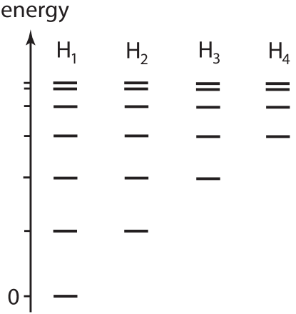
Figure 1: A generic energy spectrum for a collection of four Hamiltonians related to each other by shape invariance. The Hamiltonians are provided by the list (2.6). Note the degeneracies that exist across all the sectors.

Clearly, shape invariance is a useful tool for analyzing exactly solvable quantum mechanical systems. Why this structure should appear in some Hamiltonians and not others, however, is not clear, although given the intricacy and elegance of this structure, it would seem that there ought to be an underlying principle responsible for its appearance. As a first clue to understanding the origins of shape invariance, we note the following. While all the eigenstates of the Hamiltonians $H_{k}$ generated according to (2.6) satisfy a time-independent Schrödinger equation, which is second order, the ground state of each of these sectors satisfies a simpler, first-order equation, namely $A(g_{k})\psi_{1}(x;g_{k})=0$. Such a scenario is familiar from field theories in which there are BPS bounds. In such field theories, while the equations of motion are generically second-order equations, the field configurations that saturate BPS bounds satisfy first-order equations. We are thus led to consider the possibility that shape invariance is a manifestation of BPS-saturation. Given the close association that has been uncovered in the field theoretic context between BPS phenomena and supersymmetry algebras with a central charge, it would therefore seem natural to look for a BPS interpretation of shape invariance by considering supersymmetric quantum mechanics in which the superalgebra includes a central charge. It is this endeavor to which we now turn.

3 Supersymmetry with a Central Charge

Our goal in this paper is to determine the algebraic underpinnings of shape invariance. As we will show, supersymmetric quantum mechanics with non-vanishing central charge, while not sufficient to produce shape invariance, is a key part of the framework we seek. For now, we simply study quantum mechanics in which the superalgebra has non-vanishing central charge; the connection of such centrally extended superalgebras to shape invariance will become apparent in the subsequent section.

To develop supersymmetric quantum mechanics with a central charge, we first present the corresponding centrally-extended superalgebra. For the purposes of this paper, only the case of real central charge is relevant. The superalgebra in this case takes the form

$$\{Q,Q^{\dagger}\} = H$$

$${}[H,Q]=[H,Q^{\dagger}] = 0$$

$$\{Q,Q\}=\{Q^{\dagger},Q^{\dagger}\} = Z~{}~{}~{}.$$ (3.10)

This algebra includes the supercharges $Q$ and $Q^{\dagger}$, the real central charge $Z$, and the Hamiltonian $H$. When $Z=0$, the second condition in (3) is automatic, but for non-zero central charge, this condition must be specified independently. The above algebra implies $[Q,Z]=[Q^{\dagger},Z]=0$, as well as $H\geq|Z|$.

We wish to realize this algebra in a quantum mechanical system. Our approach is first to present an implementation of this algebra in a two-sector model, analogous to the supersymmetric quantum mechanics described in the preceding section, and then to generalize this construction to an arbitrary number of sectors.

To realize the algebra (3), we represent the supercharges as matrices

$$Q=\left(\matrix{-\eta&0\cr A&\eta}\right)\qquad,\qquad Q^{\dagger}=\left(\matrix{-\eta&A^{\dagger}\cr 0&\eta}\right)~{}~{}~{},$$ (3.11)

where $\eta$ is a real $c$-number. Then the Hamiltonian and central charge are determined by the superalgebra to be, respectively,

$$H=\left(\matrix{A^{\dagger}A+2\,\eta^{2}&0\cr 0&AA^{\dagger}+2\,\eta^{2}}\right)\qquad,\qquad Z=\left(\matrix{2\eta^{2}&0\cr 0&2\eta^{2}}\right)~{}~{}.$$ (3.12)

The operator $\Gamma=\sigma_{3}$ commutes with the Hamiltonian, and thus its eigenvalues distinguish the two sectors of the theory. Notice that the central charge has only non-negative values in this construction.

It turns out that the operators that served as supercharges when there was no central charge, namely

$$\widetilde{Q}=\left(\matrix{0&0\cr A&0}\right)~{},\qquad\widetilde{Q}^{\dagger}=\left(\matrix{0&A^{\dagger}\cr 0&0}\right)~{}~{},$$ (3.13)

still have a role to play in the centrally extended case. One notes first that $Q=\widetilde{Q}-\eta\Gamma$, and so one can write the Hamiltonian as

$$H=\{\widetilde{Q},\widetilde{Q}^{\dagger}\}+|Z|~{}~{}~{},$$ (3.14)

since $Z=\{\eta\Gamma,\eta\Gamma\}$. This makes the bound $H\geq|Z|$ manifest.

When there is non-vanishing central charge, $\{Q,\Gamma\}\neq 0$, and so the supercharges do not map states from one $\Gamma$-sector to the other $\Gamma$-sector. The operator $\widetilde{Q}$, on the other hand, not only commutes with the Hamiltonian and central charge, but also satisfies $\{\widetilde{Q},\Gamma\}=0$. Therefore, it is the operators $\widetilde{Q}$ and $\widetilde{Q}^{\dagger}$ that map states from one $\Gamma$-sector to the other. Those states for which $H>|Z|$ are doublets under this operation, while those with $H=|Z|$ are singlets.

To construct a model with $2N$ sectors for arbitrary integer $N$, one can concatenate $N$ two-sector models. To construct the supercharges, for example, one places $2\times 2$ blocks of the form (3.11) along the diagonal of a $2N\times 2N$ matrix. Upon calculating the Hamiltonian and the central charge, this procedure yields a reducible representation of the centrally extended superalgebra (3).

As an example, a four-sector model has supercharges

$$Q=\left(\begin{array}[]{cc|cc}-\eta_{1}&0&&\\ A_{1}&\eta_{1}&&\\ \hline\cr&&-\eta_{3}&0\\ &&A_{3}&\eta_{3}\end{array}\right)~{}~{},~{}~{}~{}Q^{\dagger}=\left(\begin{array}[]{cc|cc}-\eta_{1}&A_{1}^{\dagger}&&\\ 0&\eta_{1}&&\\ \hline\cr&&-\eta_{3}&A_{3}^{\dagger}\\ &&0&\eta_{3}\end{array}\right)~{}~{}.$$ (3.15)

The associated Hamiltonian $H$ and central charge $Z$ follow from (3), and are diagonal. Thus, the spectrum divides into four sectors, which we number sequentially along the diagonal. One notes that sectors 1 and 2 are degenerate, with energies bounded from below by $2\eta_{1}^{2}$, and sectors 3 and 4 are degenerate, with energies bounded from below by $2\eta_{3}^{2}$. The only exceptions to these degeneracies are that sectors 1 and 3 each have states that saturate their respective energy bounds, while the even sectors do not. Each of the degenerate pairs of sectors we dub a partnership. A typical spectrum for a four-sector model is given in Figure 2.

Figure 2: The energy spectrum of a four-sector model invariant under supersymmetry with a central charge. $H_{j}$ is the Hamiltonian for the $j^{th}$ sector. Note thtat there is no correlation between the energy levels of the first partnership (sectors 1 and 2) and those of the second partnership (sectors 3 and 4).

Once again, it is not the supercharges that swap the degenerate states within each partnership. Generalizing from the previous case, we see that the operators that swap degenerate states within a partnership are concatenations of the corresponding operators of the two-sector case; for the four-sector model, these operators are

$$\widetilde{Q}=\left(\begin{array}[]{cc|cc}0&0&&\\ A_{1}&0&&\\ \hline\cr&&0&0\\ &&A_{3}&0\end{array}\right)~{}~{},~{}~{}~{}\widetilde{Q}^{\dagger}=\left(\begin{array}[]{cc|cc}0&A_{1}^{\dagger}&&\\ 0&0&&\\ \hline\cr&&0&A_{3}^{\dagger}\\ &&0&0\end{array}\right)~{}~{}.$$ (3.16)

The generalization of this construction to the case of $2N$-sectors exhibits the essential features we have identified above. The spectrum divides into partnerships, consisting of an odd sector and the subsequent even sector. If $j$ is an odd integer, then sector $j$ and $j+1$ are bounded from below by a common constant $\eta_{j}^{2}$. The odd sector has a state with energy $\eta_{j}^{2}$ and the even sector does not, but otherwise these sectors have degenerate spectra. One can also specify generalizations of $\widetilde{Q}$, which are distinct from the supercharges, to provide the mapping between the degenerate states that reside within each partnership.

Having constructed Hamiltonians invariant under a centrally extended superalgebra, we now invoke such models in the next section, where they provide the basis for our analysis of shape invariance.

4 The Algebraic Origins of Shape Invariance

The spectrum of energy levels in supersymmetric quantum mechanics with a central charge has, in certain respects, a resemblance to the spectrum of energy levels that arises in the presence of shape invariance. For example, comparing Figures 1 and 2, each of which has a spectrum that divides into four sectors, we notice the following similarities. The states in the first sector (excepting the ground state) are degenerate with those of the second sector, just as those of third sector (excepting its lowest energy state) are degenerate with those of the fourth sector. Furthermore, the lowest energy state of each odd sector satisfies a first-order equation. The obvious generalizations of these statements hold in the case of $2N$ sectors.

However, the shape invariant case has two additional features, both of which suggest an enhanced algebraic structure. First, the same degeneracy pattern that holds within a partnership is present between the adjacent even and odd sectors of distinct partnerships. Second, as noted previously, in the shape invariant case, the lowest energy state in every sector satisifies a Bogomol’nyi-like first-order equation, something which only holds in the odd sectors for the simply supersymmetric case.

The extra degeneracies indicate the presence a symmetry operator that not only maps between degenerate levels within a partnership, but that also maps between levels from adjacent sectors that lie in distinct partnerships. Finding this operator leads, in turn, to an explanation of the Bogomol’nyi equations.

To approach this problem, we consider first the four-sector case, and then show that the results so obtained apply to the case of arbitrarily many sectors, as is necessary if we are to address shape invariance in general. Using (3.15), the four-sector Hamiltonian with centrally extended supersymmetry can be written as

$$H=\left(\matrix{A_{1}^{\dagger}A_{1}+2\,\eta_{1}^{2}&0&0&0\cr 0&A_{1}A_{1}^{\dagger}+2\,\eta_{1}^{2}&0&0\cr 0&0&A_{3}^{\dagger}A_{3}+2\,\eta_{3}^{2}&0\cr 0&0&0&A_{3}A_{3}^{\dagger}+2\,\eta_{3}^{2}\cr}\right)~{}~{}~{}.$$ (4.17)

The operator $\widetilde{Q}$ from (3.16) explains the degeneracies within each partnership that arise from the superalgebra; this suggests modifying $\widetilde{Q}$ to include an entry that maps the second sector to the third sector, and requiring that this new operator be conserved.

We therefore define the “shift operator” $S$ by

$$S\equiv\left(\matrix{0&0&0&0\cr A_{1}&0&0&0\cr 0&C&0&0\cr 0&0&A_{3}&0\cr}\right)~{}~{}~{},$$ (4.18)

and seek to determine when we can choose $C$ such that $[H,S]=0$. As we show below, the shape invariant models correspond to the case that this is possible To see this, first we impose the requirement that $[H,S]=0$, and find that this can be achieved when $A_{1}^{\dagger}A_{1}$ is shape invariant, and two auxiliary conditions are met, namely that $A_{3}$ and $A_{1}$ are related by a unitary transformation, and that $\eta_{3}$ is related to $\eta_{1}$ so that the energy levels line up suitably. Appealingly, the shape invariance condition emerges from the condition that $S$ be conserved. We then observe that one can look at this result in reverse, concluding that whenever shape invariance holds for a one-sector Hamiltonian $A_{1}^{\dagger}A_{1}$, this Hamiltonian can be embedded in a centrally extended supersymmetric quantum theory with a conserved shift operator, by defining $A_{3}$ and $\eta_{3}$ that meet the necessary conditions.

Using the matrix form of $S$ (4.18), the requirement that $H$ and $S$ commute becomes

$$A^{\dagger}_{3}A_{3}C-CA_{1}A_{1}^{\dagger}+2(\eta_{3}^{2}-\eta_{1}^{2})C=0~{}~{}~{}.$$ (4.19)

This condition suggests that there is a simple relation between $A_{1}$ and $A_{3}$. We therefore suppose that there is a unitary transformation represented by an operator $\Omega$ such that

$$A_{3}=\Omega^{\dagger}A_{1}\Omega~{}~{}~{}.$$ (4.20)

In order that we are able to make contact with shape invariance, we allow, and indeed expect, the operator $\Omega$ to implement a transformation in parameter space, mapping the $c$-number parameters of a model (such as $g$ in (2.1)) to new values, and thus altering also the values of expressions in the Hamiltonian (such as $\eta_{1}^{2}$ and $\eta_{3}^{2}$) that are functions of these parameters.

The condition that $A_{1}$ and $A_{3}$ are unitarily related can be imposed on the commutativity condition (4.19). Using a unitary operator $U$ such that $U^{2}=\Omega$, the resultant equation can be written in the form

$${\widetilde{C}}{\widetilde{A}_{1}}{\widetilde{A}_{1}^{\dagger}}-{\widetilde{A}_{1}^{\dagger}}{\widetilde{A}_{1}}{\widetilde{C}}=2({\widetilde{\eta}}_{3}^{2}-{\widetilde{\eta}}_{1}^{2}){\widetilde{C}}~{}~{},$$ (4.21)

where, for simplicity of appearance, we have introduced ${\widetilde{A}_{1}}=A_{1}U$, ${\widetilde{C}}=UC$, and ${\widetilde{\eta}}_{j}=U\eta_{j}U^{\dagger}$. Our goal is to find a value for ${\widetilde{C}}$ that will lead to a solution of (4.21). The ansatz with which we have found success is to choose ${\widetilde{C}}={\widetilde{A}_{1}}$ (that is, $C=U^{\dagger}A_{1}U$), turning the conservation condition (4.21) into

$$\{\,{\widetilde{A}_{1}}\,,\,[\,{\widetilde{A}_{1}}\,,\,{\widetilde{A}_{1}^{\dagger}}\,]\,\}=2({\widetilde{\eta}}_{3}^{2}-{\widetilde{\eta}}_{1}^{2}){\widetilde{A}_{1}}~{}~{}.$$ (4.22)

Thus, to achieve conservation of $S$, the left side of (4.22) must be proportional to ${\widetilde{A}_{1}}$. We note that this condition is satisfied if there is a $c$-number $\kappa$ such that

$$[\,{\widetilde{A}_{1}}\,,\,{\widetilde{A}_{1}^{\dagger}}\,]=\kappa~{}~{}~{}.$$ (4.23)

Combining (4.23) with (4.22), one finds $\{\kappa,{\widetilde{A}_{1}}\}=2({\widetilde{\eta}}_{3}^{2}-{\widetilde{\eta}}_{1}^{2}){\widetilde{A}_{1}}$. Rewriting this in terms of the original quantities, remembering that $U$ does not commute with $\kappa$, this relationship takes the form

$$\kappa+U^{\dagger}\kappa U=2(\eta_{3}^{2}-\eta_{1}^{2})~{}~{}.$$ (4.24)

When this condition holds, the requirement that $S$ commute with $H$ is satisfied.

It is useful re-phrase the above results in reverse. Suppose that $A_{1}^{\dagger}A_{1}$ is shape invariant. Then $A_{1}$ satisfies

$$A_{1}A_{1}^{\dagger}-U^{\dagger}A_{1}^{\dagger}A_{1}U=\kappa~{}~{}~{},$$ (4.25)

where $\kappa$ is a $c$-number and $U$ implements a shift in the parameter(s) of the theory, which is precisely the statement (4.23). With this condition satisfied, it is possible to construct a multiple sector model that has $H_{1}=A_{1}^{\dagger}A_{1}+2\eta_{1}^{2}$ as the Hamiltonian in its first sector, and that is invariant under both a centrally extended superalgebra and a shift operator $S$. To obtain this mult-sector theory, one defines quantities $A_{3}$ and $\eta_{3}$, respectively, by

$$A_{3} = (U^{\dagger})^{2}A_{1}(U)^{2}$$

$$2\eta_{3}^{2} = 2\eta_{1}^{2}+\kappa+U^{\dagger}\kappa U~{}~{}.$$ (4.26)

The conserved shift operator takes the form

$$S=\left(\matrix{0&0&0&0\cr A_{1}&0&0&0\cr 0&U^{\dagger}A_{1}U&0&0\cr 0&0&{U^{\dagger}}^{2}A_{1}{U}^{2}&0}\right)~{}~{},$$ (4.27)

while the Hamiltonian for the second sector can be written as $(U^{\dagger}A_{1}U)^{\dagger}(U^{\dagger}A_{1}U)+\eta_{1}^{2}+\kappa$. In this way, one sees that the shape invariant theories correspond to centrally extended supersymmetric theories with a conserved shift operator.

It is now straightforward to generalize this construction from the four sector case to a model with an arbitrary number of sectors. Since, due to (4.25) and (4.27), the relationship between sector $j$ and sector $j+1$ is implemented in the same way for each value of $j$ (and not just when the sectors $j$ and $j+1$ fall within a single partnership), the algebraic structure found above can be readily extended to a theory with $2N$ sectors, where $N$ is an arbitrary integer. For notational compactness, it helps to define the diagonal matrix ${\bf U}={\rm diag}(1,U,U^{2},U^{3},\ldots,U^{2N-1})$ and the matrix, all of whose entries lie just below the diagonal, ${{\bf A}}_{i,j}=A_{1}\delta_{i,j+1}$. Then in the $2N$ sector model, the shift operator (that is, the extra conserved quantity) takes the form

$$S=U{\bf U}^{\dagger}{\bf A}{\bf U}~{}~{}~{},$$ (4.28)

and it is conserved provided $A_{1}A_{1}^{\dagger}-U^{\dagger}A_{1}^{\dagger}A_{1}U=\kappa$, i.e., provided that $A_{1}^{\dagger}A_{1}$ is shape invariant. Thus, shape invariance corresponds to the invariance of the multiple-sector Hamiltonian under the action of the shift operator $S$.

It is worth noting that conservation of $S$ plays a role here analogous to that played by the LaPlace-Runge-Lenz vector in the hydrogen atom. In the hydrogen atom, spherical symmetry dictates that the energy eigenvalues depend on a radial quantum number $n$ and an angular momentum quantum number $\ell$. The additional conservation law associated with the LaPlace-Runge-Lenz vector ensures that states with the same $n$ value but different $\ell$ values are in fact degenerate [3]. Likewise, when a model is invariant under a centrally extended superalgebra, this algebra imposes no relation between the energy levels of the different partnerships; it is conservation of the shift operator that aligns these partnerships to produce the additional degeneracies that arise in the presence of shape invariance.

The example in the appendix shows briefly how the structure we have derived above applies to a particular case.

5 Shape Invariance, BPS, and the Shift Operator

Having obtained the shape invariance condition from the algebra of centrally extended supersymmetry enhanced by a shift operator, we now consider the further implications of this algebra. For convenience, we again consider initially the four-sector model. In this case, all states in the fourth sector are trivially annihilated by $S$. However, in the other three sectors, something more interesting occurs.

Due to (4.17), (4.25), and (4), the Hamiltonian of the four-sector model is related to $S$ in an especially simple way. In particular,

$$H=S^{\dagger}S+B~{}~{},$$ (5.29)

where $B$ is a diagonal matrix that, except in its final entry, consists entirely of $c$-numbers. One readily determines that

$$B=\left(\matrix{2\eta_{1}^{2}&0&0&0\cr 0&2\eta_{1}^{2}+\kappa&0&0\cr 0&0&2\eta_{1}^{2}+\kappa+U^{\dagger}\kappa U&0\cr 0&0&0&H_{4}\cr}\right)~{}~{}~{}.$$ (5.30)

In the first three sectors, the energies are constrained by a Bogomol’nyi bound, $H_{k}\geq(B)_{kk}$. This bound is saturated only for a state annihilated by $S$; $S$ is a first-order differential operator, and this annihilation condition then is the Bogomol’nyi equation for these BPS-saturating states. These states are the ground states of the first three sectors.

If we consider the full four-sector theory, the identity $S^{4}=0$ implies that a typical multiplet of degenerate states consists of four states. The multiplets in which one of the states from the first three sectors satifies $S\psi=0$ are shortened, however, with one, two, and three states, respectively. This is analogous to what occurs for BPS-saturating states when it is the supercharge involved in the annihilation condition [7] [8].

Finally, because each of the first three states of the first sector have to be degenerate with the Bogomol’nyi-saturating ground state of one of the first three sectors, the constants in $B$ represent not only the Bogomol’nyi bounds of the various sectors, but also the first three energy eigenvalues of the original Hamiltonian.

Of course, nothing is special about the four-sector model; we can easily extend these results to a theory with an arbitrary number of sectors. In a model with $2N$ sectors, the BPS structure still holds, with $S$ defined as in (4.28), and

$$H = S^{\dagger}S+B$$

$$B = {\rm diag}(b_{1},b_{2},\ldots,b_{2N-1},H_{2n})$$

$$b_{1} = 2\eta_{1}^{2}$$

$$b_{j+1} = b_{j}+(U^{\dagger})^{j-1}\kappa U^{j-1}~{}~{}~{}.$$ (5.31)

In the first $2N-1$ sectors, the ground state saturates a Bogomol’nyi bound $H=B$ (that is, has energy $b_{j}$), and this state is annihilated by the first-order differential operator $S$. Because of the degeneracies produced by conservation of $S$, these Bogomol’nyi bound values are also the energies of the first $2N-1$ states of $H_{1}$. These $2N-1$ lowest energy states of $H_{1}$ are part of shortened $S$ multiplets (since $S^{2N}=0$, multiplets of length $2N$ are the norm); the $j^{th}$ energy level of $H_{1}$ can be obtained by applying $S^{\dagger}$ repeatedly to the Bogomol’nyi-saturating ground state of the $j^{th}$ sector. While for any finite value of $2N$, the BPS structure only applies to the first $2N-1$ sectors and energy levels, this is not a fundamental limitation; as the whole process can be iterated for arbitrarily large values of $2N$, in fact all the energy levels of $H_{1}$ (and, indeed, of the Hamiltonians with which it is associated via shape invariance) fit into this algebraic framework.

This completes the analysis of the structure of shape invariance.

6 Summary and Prospects

We have demonstrated that shape invariance is associated with a more comprehensive invariance algebra: supersymmetry with a central charge, enhanced by the addition of a shift operator $S$ that maps among adjacent sectors of the supersymmetric model, even when those sectors come from distinct partnerships. Most compellingly, there turns out to be a natural BPS interpretation of shape invariance due to this structure. When the shift operator is conserved, and hence shape invariance holds, the Hamiltonian can be written as $H=S^{\dagger}S+B$, and so not only is $H\geq B$, but the states for which $H=B$ are the states annihilated by $S$; the equation $S\psi=0$ is nothing but the Bogomol’nyi equation for this model. Finally, in a result that exceeds conventional BPS results, because $S$ plays a role analogous to a LaPlace-Runge-Lenz vector, it imposes degeneracies between every pair of adjacent sectors, and thus the eigenvalues of $B$ are also the energy eigenvalues of the first sector, and the corresponding states can be obtained by the action of $S^{\dagger}$ on the BPS-saturating states.

The algebra we have described gives a natural framework for understanding the origins of shape invariance. Still, it is a curious question as to whether these Bogomol’nyi bounds can be given a natural topological explanation [8], with each sector in the shape invariant case corresponding to a distinct topological sector. We have pursued some initial efforts in this direction, by using a field theoretic approach to study supersymmetric quantum mechanics with a central charge [9]. In the context of the sigma models we have studied in that language, shape invariance amounts to a restriction on the target space geometry. Continued efforts should show if there is additional significance to such a restriction, and whether there is a natural way to interpret the rest of the algebraic structure described above in terms of features of the target space. We believe such an approach has the potential to lead us to a topological interpretation of the construction presented in this paper.

Acknowledgments

We thank Ted Allen for his generous ear and insightful observations, and Costas Efthimiou for his helpful comments on the manuscript.

Appendix A Appendix

As an example of shape invariance, consider the Hamiltonian

$$H=-{d^{2}\over dx^{2}}+{b\,{\rm sech}^{2}(x)}~{}~{}.$$ (A.32)

Setting

$$A={d\over dx}+g\,{\rm tanh}(x)~{}~{},$$ (A.33)

one obtains the paired Hamiltonians

$$H_{1}(g)=A^{\dagger}A=-{d^{2}\over dx^{2}}-g(g+1)\,{\rm sech}^{2}(x)+g^{2}$$ (A.34)

and

$$H_{2}(g)=AA^{\dagger}=-{d^{2}\over dx^{2}}-g(g-1)\,{\rm sech}^{2}(x)+g^{2}~{}~{}.$$ (A.35)

Clearly, $H_{2}(g)=H_{1}(g-1)+(2\,g-1)$, which is an explicit manifestation of the shape invariance condition (2.5), recovered in our construction by (4.25).

To identify the necessary unitary transformation called for in our analysis, note that $U^{\dagger}f(g)U$ must yield $f(g-1)$. Such a shift is achieved by the operator

$$U=\exp(\partial/\partial g)~{}~{}.$$ (A.36)

The parameter $\kappa$ associated with this model is $\kappa(g)=2\,g-1$. The interested reader can easily apply the rest of our construction to this example.

References

-
[1]
L.Infeld and T.D.Hull,
Rev. Mod. Phys 23 (1951) 21;
L.Gendenshtein, JETP Lett. 38 (1983) 356;
F.Cooper, J.N.Ginocchio and A.Khare, Phys. Rev. D36 (1986) 2485;
F. Cooper, A. Khare, and U.Sukhatme, Phys. Rept. 251 (1995) 267. - [2] E. Witten, Nucl. Phys. B188 (1981) 513.
-
[3]
P.-S. LaPlace, Traité du Mécanique Cèleste, 1799;
W. Pauli, Z. Physik 36 (1926) 336;
H. Goldstein, Am. J. Phys. 43 (1975) 745;
H. Goldstein, Am. J. Phys. 44 (1976) 1123. -
[4]
E.B. Bogomol’nyi, Sov. J. Nucl. Phys.
24 (1976) 449;
M.K. Prasad and C.H. Sommerfield, Phys. Rev. Lett. 35 (1975) 760;
R. Rajaraman, Solitons and Instantons, Amsterdam: North-Holland, 1987. - [5] E. Witten, Nucl. Phys. B202 (1982) 253.
- [6] To see examples of this very different phenomenon, one can turn to the Tarnhelm in R. Wagner, Der Ring des Nibelungen; the Chameleon in S. Lee, Spider-Man; and Lt. Odo in G. Roddenberry, Star Trek: Deep Space Nine.
- [7] A. Salam and J. Strathdee, Nucl. Phys. B80 (1974) 499.
- [8] E. Witten and D. Olive, Phys. Lett. B78 (1978) 97.
- [9] M. Faux and D. Spector, Duality and Central Charges in Supersymmetric Quantum Mechanics, hep-th/0311095.