Generalized reduction criterion for separability of quantum states

Abstract

A new necessary separability criterion that relates the structures of the total density matrix and its reductions is given. The method used is based on the realignment method [K. Chen and L.A. Wu, Quant. Inf. Comput. 3, 193 (2003)]. The new separability criterion naturally generalizes the reduction separability criterion introduced independently in previous work of [M. Horodecki and P. Horodecki, Phys. Rev. A 59, 4206 (1999)] and [N.J. Cerf, C. Adami and R.M. Gingrich, Phys. Rev. A 60, 898 (1999)]. In special cases, it recovers the previous reduction criterion and the recent generalized partial transposition criterion [K. Chen and L.A. Wu, Phys. Lett. A 306, 14 (2002)]. The criterion involves only simple matrix manipulations and can therefore be easily applied.

I Introduction

In the last decade quantum entangled states have showed remarkable applications and become one of the key resources in the rapidly expanding field of quantum information processing. The history can be traced back to the earlier well-known papers of Einstein, Podolsky and Rosen EPR35 , Schrödinger Sch35 and Bell Bell64 . Recently quantum teleportation, quantum cryptography, quantum dense coding and parallel computation pre98 ; nielsen ; zeilinger have spurred a flurry of activity in the effort to fully exploit the potential of quantum entanglement. Despite of its importance, we do not yet have a full understanding of the physical character and mathematical structure for entangled states. We even do not know completely wether a generic quantum state is entangled, and how much entanglement remained after some noisy quantum processes.

A state of a composite quantum system is said to be disentangled or separable if it can be prepared in a “local” or “classical” way. A separable bipartite system can be prepared as an ensemble realization of pure product states $\left|\psi_{i}\right\rangle_{A}\left|\phi_{i}\right\rangle_{B}$ ($i=1,...,M$ for some positive integer $M$) occurring with a certain probability $p_{i}$:

$$\rho_{AB}=\sum_{i}p_{i}\rho_{i}^{A}\otimes\rho_{i}^{B},$$ (1)

where $\rho_{i}^{A}=\left|\psi_{i}\right\rangle_{A}\left\langle\psi_{i}\right|$, $\rho_{i}^{B}=\left|\phi_{i}\right\rangle_{B}\left\langle\phi_{i}\right|$, $\sum_{i}p_{i}=1$ and $\left|\psi_{i}\right\rangle_{A}$, $\left|\phi_{i}\right\rangle_{B}$ are normalized pure states of the subsystems $A$ and $B$, respectively werner89 . If no convex linear combination exists for a given $\rho_{AB}$, the state is called “entangled” and includes quantum correlation.

For a pure state $\rho_{AB}$, it is straightforward to judge its separability: a pure state $\rho_{AB}$ is separable if and only if there is only one item in Eq. (1) and $\rho^{A}$ resp. $\rho^{B}$ are the reduced density matrices defined as $\rho^{A}=Tr_{B}(\rho_{AB})$ and $\rho^{B}=Tr_{A}(\rho_{AB})$. However, for a generic mixed state $\rho_{AB}$, finding a decomposition like in Eq. (1) or proving that it does not exist is a non-trivial task (we refer to recent good reviews lbck00 ; terhal01 ; 3hreview and references therein). There has been considerable effort in recent years to analyze the separability and quantitative character of quantum entanglement. The Bell inequalities satisfied by a separable system give the first necessary condition for separability Bell64 . Many years after the appearance of Bell inequalities, Peres made an important step forward in 1996 by showing that partial transpositions with respect to one and more subsystems of the density matrix for a separable state are positive,

$$\rho^{T_{\mathcal{X}}}\geq 0,$$ (2)

where $\mathcal{X}$ is either $A$ or $B$, $\rho^{T_{\mathcal{X}}}$ stands for the partial transpose with respect to $\mathcal{X}$. Thus $\rho^{T_{\mathcal{X}}}$ should have non-negative eigenvalues (this is known as the $PPT$ criterion or Peres-Horodecki criterion) peres , which was further shown by Horodecki et al. 3hPLA223 to be sufficient for $2\times 2$ and $2\times 3$ bipartite systems. Meanwhile, these authors also found a necessary and sufficient condition for separability by establishing a close connection between positive map theory and separability 3hPLA223 . In view of the quantitative character for entanglement, Wootters succeeded in computing the “entanglement of formation” be96 and thus obtained a separability criterion for $2\times 2$ mixtures wo98 . The “reduction criterion” proposed independently in 2hPRA99 and cag99 gives another necessary criterion which is equivalent to the $PPT$ criterion for $2\times n$ composite systems but is generally weaker. Pittenger et al. gave also a sufficient criterion for separability connected with the Fourier representations of density matrices Rubin00 . Later, Nielsen et al. nielson01 presented another necessary criterion called the majorization criterion: the decreasingly ordered vector of the eigenvalues for $\rho_{AB}$ is majorized by that of $\rho_{A}$ or $\rho_{B}$ alone for a separable state. A new method of detecting entanglement called entanglement witnesses was given in 3hPLA223 and ter00 ; lkch00 . Some necessary and sufficient criteria of separability for low rank cases of the density matrix are also known hlvc00 ; afg01 ; feipla02 . In addition, it was shown in wu00 and pxchen01 that a necessary and sufficient separability criterion is also equivalent to certain sets of equations. A PPT extension based on semidefinite programs is proposed in dps which can test numerically the separability.

However, despite these advances, practical and easily computable criteria for a generic bipartite system are mainly limited to several ones such as the $PPT$, reduction, majorization criteria as well as the PPT extension. Very recently Rudolph ru02 and K. Chen and L.A. Wu ChenQIC03 proposed a new operational criterion for separability: the realignment criterion (named following the suggestion of Horo02 , it coincides with the computational cross norm criterion given in Ref. ru02 ). The criterion is very simple to apply and shows dramatic ability to detect many of the bound entangled states ChenQIC03 and even genuinely tripartite entanglement Horo02 . Soon after the appearance of ChenQIC03 , Horodecki et al. showed that the $PPT$ criterion and realignment criterion are equivalent to the permutations of the density matrix’s indices Horo02 . A simple single framework for these criteria for the multipartite case in any dimensions was recently given in chenPLA02 and is called the generalized partial transposition criterion (GPT) which includes, as special cases, the Peres-Horodecki criterion (PPT), the realignment criterion and the permutation indices criterion for density matrix. Some further properties of the realignment criterion have been very recently derived in ru0212047 .

In this paper we present a systematic generalization of the reduction criterion employing a realignment technique of a certain matrix constructed from the density matrix. This criterion includes the reduction criterion and the GPT criterion as special cases. It unifies them in a single simple framework. Thus our criterion is a strong separability test for a generic bipartite or even for multipartite quantum states in arbitrary dimensions. The detailed constructions are given in Section II where the reduction and the GPT criteria are shown to be two special cases of our new criterion. Some interesting examples are given in Section III. A brief summary and some discussions are given in the last section.

II The criteria for separability

In this section we study the separability of the density matrix for any bipartite system in arbitrary finite dimension. Motivated by the reduction criterion and the Kronecker product approximation technique loan ; pits , we give a new separability criterion by analyzing the trace norm for some realigned version of a matrix constructed from the whole density matrix and its reduced ones.

II.1 Some notation

We first introduce some notations used in various matrix operations (see e.g., hornt1 ; hornt ):

Definition: For any $m\times n$ matrix $A=[a_{ij}]$, with entries $a_{ij}$, we define a vector $\mathcal{V}_{vec}(A)$ by

$$\mathcal{V}_{vec}(A)=[a_{11},\cdots,a_{m1},a_{12},\cdots,a_{m2},\cdots,a_{1n},\cdots,a_{mn}]^{t},$$

where $t$ represents the standard transposition operation. Let $\mathcal{T}_{r}$ (resp. $\mathcal{T}_{c}$) denote the row transposition (resp. column transposition) of $A$:

$$\mathcal{T}_{r}(A) =(\mathcal{V}_{vec}(A))^{t},$$ (3)

$$\mathcal{T}_{c}(A) =\mathcal{V}_{vec}(A).$$ (4)

It is easily verified that

$$\mathcal{T}_{c}\mathcal{T}_{r}(A)=\mathcal{T}_{r}\mathcal{T}_{c}(A)=A^{t}.$$ (5)

For example, for a $2\times 2$ matrix $A$,

$$A=\left(\begin{array}[]{cc}a_{11}&a_{12}\\ a_{21}&a_{22}\end{array}\right),$$

we have

$$\mathcal{T}_{r}(A) =\left(\begin{array}[]{cc|cc}a_{11}&a_{21}&a_{12}&a_{22}\end{array}\right),$$ (7)

$$\mathcal{T}_{c}(A) =\left(\begin{array}[]{c}a_{11}\\ a_{21}\\ \hline\cr a_{12}\\ a_{22}\end{array}\right).$$ (12)

For a generic matrix $A={\displaystyle\sum\limits_{i,j}}A_{ij}\left|i\right\rangle\left\langle j\right|={\displaystyle\sum\limits_{i,j}}A_{ij}\left|i\right\rangle\otimes\left\langle j\right|={\displaystyle\sum\limits_{i,j}}A_{ij}\left\langle j\right|\otimes\left|i\right\rangle$, where $\left|i\right\rangle,\left|j\right\rangle$ are vectors of a suitably selected normalized orthogonal basis, $\left\langle i\right|,\left\langle j\right|$ are the corresponding transpositions (not conjugate transpositions). Under the operations $\mathcal{T}_{r}$ and $\mathcal{T}_{c}$ one has:

$$A\overset{\mathcal{T}_{r}}{\longrightarrow}{\displaystyle\sum\limits_{i,j}}A_{ij}\left\langle j\right|\otimes\left\langle i\right|\overset{\mathcal{T}_{c}}{\longrightarrow}{\displaystyle\sum\limits_{i,j}}A_{ij}\left|j\right\rangle\otimes\left\langle i\right| =A^{t},$$ (13)

$$A\overset{\mathcal{T}_{c}}{\longrightarrow}{\displaystyle\sum\limits_{i,j}}A_{ij}\left|j\right\rangle\otimes\left|i\right\rangle\overset{\mathcal{T}_{r}}{\longrightarrow}{\displaystyle\sum\limits_{i,j}}A_{ij}\left|j\right\rangle\otimes\left\langle i\right| =A^{t}.$$ (14)

We further define $\mathcal{T}_{r_{k}}$ (resp. $\mathcal{T}_{c_{k}}$) ($k=A,B$) to be the row (resp. column) transposition with respect to the subsystems $A,B$. We set $\mathcal{T}_{\{x_{1},x_{2},...\}}\equiv\mathcal{T}_{x_{1}}\mathcal{T}_{x_{2}}...$ for $x_{1},~{}x_{2}\in\{r_{A},c_{A},r_{B},c_{B}\}$. A generalized partial transposition operation (GPT operation) for a bipartite density matrix is thus given by $\mathcal{T}_{\mathcal{Y}}$, $\mathcal{Y}\subset\{r_{A},c_{A},r_{B},c_{B}\}$, where $\mathcal{T}_{\mathcal{Y}}$ stands for all partial transpositions contained in $\mathcal{Y}$ which is a subset of $\{r_{A},c_{A},r_{B},c_{B}\}$. With these notations, the realignment criterion can easily be stated. For example, for a bipartite system, we only need to make partial transpositions with respect to $\mathcal{Y}=\{c_{A},r_{B}\}$. This is equivalent to the realignment operation given in ru02 and ChenQIC03 , for the proof, see chenPLA02 .

We also need the following result in matrix analysis. Let $Z$ be an $m\times m$ block matrix with block size $n\times n$. We define a realigned matrix $\widehat{Z}$ of size $m^{2}\times n^{2}$ that contains the same elements as in $Z$ but in different positions,

$$\widehat{Z}=\left[\begin{array}[c]{c}\mathcal{V}_{vec}(Z_{1,1})^{t}\\ \vdots\\ \mathcal{V}_{vec}(Z_{m,1})^{t}\\ \vdots\\ \mathcal{V}_{vec}(Z_{1,m})^{t}\\ \vdots\\ \mathcal{V}_{vec}(Z_{m,m})^{t}\end{array}\right].$$ (15)

$\widehat{Z}$ has the singular value decompositions:

$$\widehat{Z}=U\Sigma V^{\dagger}=\sum_{i=1}^{q}\sigma_{i}u_{i}v_{i}^{\dagger},$$ (16)

where $U=[u_{1}u_{2}\cdots u_{m^{2}}]\in\ \hbox{\vrule width=0.6pt,height=6.5pt,depth=0.0pt\hskip-3.2pt}C^{m^{2}\times m^{2}}$ and $V=[v_{1}v_{2}\cdots v_{n^{2}}]\in\ \hbox{\vrule width=0.6pt,height=6.5pt,depth=0.0pt\hskip-3.2pt}C^{n^{2}\times n^{2}}$ are unitary matrices, $\Sigma$ is a diagonal matrix with elements $\sigma_{1}\geq\sigma_{2}\geq\cdots\geq\sigma_{q}\geq 0$ and $q\equiv\min(m^{2},n^{2})$. In fact, the number of nonzero singular values $\sigma_{i}$ is the rank $r$ of the matrix $\widehat{Z}$, and $\sigma_{i}$ are exactly the nonnegative square roots of the eigenvalues of $\widehat{Z}\widehat{Z}^{\dagger}$ or $\widehat{Z}^{\dagger}\widehat{Z}$ hornt . Based on the above constructions, $Z$ can be expressed as:

$$Z=\sum_{i=1}^{r}(X_{i}\otimes Y_{i}),$$ (17)

with $\mathcal{V}_{vec}(X_{i})=\sqrt{\sigma_{i}}u_{i}$ and $\mathcal{V}_{vec}(Y_{i})=\sqrt{\sigma_{i}}v_{i}^{\ast}$ loan ; pits .

II.2 The generalized reduction criterion for separability

We now derive the main result of this paper: a generalized reduction criterion for separability of bipartite quantum systems in arbitrary dimensions.

II.2.1 The main theorem

The reduction criterion given in 2hPRA99 and cag99 says that for any bipartite $m\times n$ separable states, the following inequalities should be satisfied simultaneously:

$$\mathbb{I}_{m}\otimes\rho_{B}-\rho_{AB}\geqslant 0,\text{ \ \ \ \ \ }\rho_{A}\otimes\mathbb{I}_{n}-\rho_{AB}\geqslant 0,$$ (18)

where $\rho_{A,B}$ are the reduced density matrixes with respect to the subsystems $A$ and $B$, $\mathbb{I}_{m}$ (resp. $\mathbb{I}_{n}$) is an $m$ (resp. $n$) dimensional identity matrix. This criterion is shown to be equivalent to the PPT criterion for $2\times n$ system but it is generally weaker than the PPT criterion 2hPRA99 ; cag99 . So it certainly cannot detect any bound entangled states which are PPT. Noticing this fact and the powerful ability of the realignment criterion, in particular its generalization: the GPT criterion, we expect that some stronger test may appear. The reduction criterion is in essence a positive map. Combining the technique for this positive map and the Kronecker product approximation technique for a matrix loan ; pits , we apply a more general map:

$$\rho_{AB}\longrightarrow\widetilde{\rho_{AB}}=ab\mathbb{I}_{mn}-a\mathbb{I}_{m}\otimes\rho_{B}-b\rho_{A}\otimes\mathbb{I}_{n}+\rho_{AB},$$ (19)

where $a,~{}b$ are arbitrary complex numbers. We are going to derive a necessary separability condition of $\rho_{AB}$ in terms of the trace norm (Ky Fan norm) of a matrix obtained from a $GPT$ map on $\widetilde{\rho_{AB}}$. The trace norm of a matrix $Z$ is a unitary invariant norm which is defined as the sum of all the singular values of $Z$, or alternatively the sum of the nonnegative square roots of the eigenvalues of $ZZ^{\dagger}$ or $Z^{\dagger}Z$. We thus arrive at the following separability criterion for a bipartite system:

Theorem: If a bipartite density matrix $\rho_{AB}$ defined on an $m\times n$ space is separable, then the generalized reduction version $\widetilde{\rho_{AB}}$ of $\rho_{AB}$ should satisfy

$$||\widetilde{\rho_{AB}}^{\mathcal{T}_{\mathcal{Y}}}||\leq h_{a}h_{b},~{}~{}~{}~{}~{}~{}\forall\mathcal{Y}\subset\{r_{A},c_{A},r_{B},c_{B}\},$$ (20)

where $\mathcal{T}_{r_{k}}$ or $\mathcal{T}_{c_{k}}$ ($k=A,B$) stands for transpositions with respect to the row or column for the subsystem $k$. The numbers $h_{a},h_{b}$ are defined by

$$\begin{array}[]{l}\begin{array}[]{l}h_{a}\equiv\\ \left\{\begin{array}[]{ll}|a-1|+(m-1)|a|,&r_{A},c_{A}\in\mathcal{Y}\text{\ or }~{}r_{A},c_{A}\notin\mathcal{Y},\\ (|a-1|^{2}+(m-1)|a|^{2})^{\frac{1}{2}},&r_{A}\in\mathcal{Y},~{}c_{A}\notin\mathcal{Y}\text{\ or}\\ &c_{A}\in\mathcal{Y},~{}r_{A}\notin\mathcal{Y},\end{array}\right.\end{array}\\ \begin{array}[]{l}h_{b}\equiv\\ \left\{\begin{array}[]{ll}|b-1|+(n-1)|b|,&r_{B},c_{B}\in\mathcal{Y}\text{\ or }~{}r_{B},c_{B}\notin\mathcal{Y},\\ (|b-1|^{2}+(n-1)|b|^{2})^{\frac{1}{2}},&r_{B}\in\mathcal{Y},~{}c_{B}\notin\mathcal{Y}\text{\ or }\\ &c_{B}\in\mathcal{Y},~{}r_{B}\notin\mathcal{Y},\end{array}\right.\end{array}\end{array}$$

where $a,~{}b\in\ \hbox{\vrule width=0.6pt,height=6.5pt,depth=0.0pt\hskip-3.2pt}C$, $\mathcal{T}_{\mathcal{Y}}$ represents partial transpositions with respect to every element contained in the set $\mathcal{Y}$ of the related subsystems.

Proof: We only need to find the bound for the trace norm of $||\widetilde{\rho_{AB}}^{\mathcal{T}_{\mathcal{Y}}}||$ with respect to some operations $\mathcal{T}_{\mathcal{Y}}$ for any separable states. Considering a separable bipartite system, we suppose $\rho_{AB}$ has a decomposition, $\rho_{AB}=\sum_{i}p_{i}\rho_{i}^{A}\otimes\rho_{i}^{B}$ with $0\leq p_{i}\leq 1$, $\sum_{i}p_{i}=1$. Under map (19) it is evident that

$$\begin{array}[]{rcl}\rho_{AB}\rightarrow\widetilde{\rho_{AB}}&=&ab\mathbb{I}_{mn}-a\mathbb{I}_{m}\otimes\rho_{B}-b\rho_{A}\otimes\mathbb{I}_{n}+\rho_{AB}\\ &=&\sum_{i}p_{i}(a\mathbb{I}_{m}-\rho_{i}^{A})\otimes(b\mathbb{I}_{n}-\rho_{i}^{B}),\end{array}$$

where $\rho_{A}$ and $\rho_{B}$ are the reduced density matrixes defined by $\rho_{A}\equiv Tr_{B}(\rho_{AB})=\sum_{i}p_{i}\rho_{i}^{A}$, $\rho_{B}\equiv Tr_{A}(\rho_{AB})=\sum_{i}p_{i}\rho_{i}^{B}$. We have

$$\rho_{i}^{A}\otimes\rho_{i}^{B}$$

$$= U_{i}\left(\begin{array}[]{cccc}1&&&\\ &0&&\\ &&\ddots&\\ &&&0\end{array}\right)_{m}U_{i}^{{\dagger}}\otimes V_{i}\left(\begin{array}[]{cccc}1&&&\\ &0&&\\ &&\ddots&\\ &&&0\end{array}\right)_{n}V_{i}^{{\dagger}},$$

where we have diagonalized the (rank one) density matrix $\rho_{i}^{A}$ (resp. $\rho_{i}^{B})$ with the $m$ (resp. $n$)-dimensional unitary matrix $U_{i}$ (resp. $V_{i}$). It is straightforward to check that

$$(a\mathbb{I}_{m}-\rho_{i}^{A})\otimes(b\mathbb{I}_{n}-\rho_{i}^{B})=U_{i}\mathcal{A}U_{i}^{{\dagger}}\otimes V_{i}\mathcal{B}V_{i}^{{\dagger}},$$ (22)

where $\mathcal{A}$ and $\mathcal{B}$ are diagonal matrices:

$$\mathcal{A}=\left(\begin{array}[]{cccc}a-1&&&\\ &a&&\\ &&\ddots&\\ &&&a\end{array}\right)_{m},~{}\mathcal{B}=\left(\begin{array}[]{cccc}b-1&&&\\ &b&&\\ &&\ddots&\\ &&&b\end{array}\right)_{n}.$$

For an $m\times m$ (resp. $n\times n$) matrix $P$ (resp. $Q$) acting on the complex space associated to the subsystem $A$ (resp. $B$), the trace norm of the matrices $P$ and $Q$ has the property: $||P\otimes Q||=||P||\cdot||Q||$. And for any matrices $X,~{}Y~{}Z$ acting on the subsystem $A$ (or $B$), the $\mathcal{V}_{vec}$ operations have the property: $\mathcal{V}_{vec}(XYZ)=(Z^{T}\otimes X)\mathcal{V}_{vec}(Y)$, where both sides are column vectors and the tensor operation $\otimes$ has nothing to do with different subspaces $A$ and $B$ hornt .

Let $\widetilde{\rho_{AB}}^{\mathcal{T}_{\mathcal{Y}}}$ denote the transformed matrix of $\widetilde{\rho_{AB}}$ under the partial transposition ${\mathcal{T}_{\mathcal{Y}}}$. Without loss of generality we suppose that we only make a row transposition to the subsystem $A$. According to (3), we have

$$(U_{i}\mathcal{A}U_{i}^{{\dagger}}\otimes V_{i}\mathcal{B}V_{i}^{{\dagger}})^{\mathcal{T}_{\{r_{A}\}}}$$ (23)

$$= (\mathcal{V}_{vec}(U_{i}\mathcal{A}U_{i}^{{\dagger}}))^{t}\otimes V_{i}\mathcal{B}V_{i}^{{\dagger}}$$

$$= (\mathcal{V}_{vec}(\mathcal{A}))^{t}(U_{i}{}^{{\dagger}}\otimes U_{i}^{t})\otimes V_{i}\mathcal{B}V_{i}^{{\dagger}}.$$

In terms of the unitary invariant property of the trace norm we obtain

$$||(U_{i}\mathcal{A}U_{i}^{{\dagger}}\otimes V_{i}\mathcal{B}V_{i}^{{\dagger}})^{\mathcal{T}_{\{r_{A}\}}}||$$

$$= ||(\mathcal{V}_{vec}(\mathcal{A}))^{t}(U_{i}{}^{{\dagger}}\otimes U_{i}^{t})||\cdot||V_{i}\mathcal{B}V_{i}^{{\dagger}}||$$

$$= ||(\mathcal{V}_{vec}(\mathcal{A}))^{t}||\cdot||\mathcal{B}||$$

$$= (|a-1|^{2}+(m-1)|a|^{2})^{\frac{1}{2}}(|b-1|+(n-1)|b|).$$

Using the convex property of the trace norm, we get

$$||\widetilde{\rho_{AB}}^{\mathcal{T}_{\{r_{A}\}}}||$$ (24)

$$= ||\sum_{i}p_{i}(U_{i}\mathcal{A}U_{i}^{{\dagger}}\otimes V_{i}\mathcal{B}V_{i}^{{\dagger}})^{\mathcal{T}_{\{r_{A}\}}}||$$

$$\leq (\sum_{i}p_{i})(|a-1|^{2}+(m-1)|a|^{2})^{\frac{1}{2}}(|b-1|+(n-1)|b|)$$

$$= (|a-1|^{2}+(m-1)|a|^{2})^{\frac{1}{2}}(|b-1|+(n-1)|b|).$$

A corresponding procedure can be applied for the column transposition to the subsystem $A$ and corresponding operations for the subsystem $B$:

$$||\widetilde{\rho_{AB}}^{\mathcal{T}_{\{c_{A}\}}}||$$

$$\leq (|a-1|^{2}+(m-1)|a|^{2})^{\frac{1}{2}}\cdot(|b-1|+(n-1)|b|),$$

$$||\widetilde{\rho_{AB}}^{\mathcal{T}_{\{r_{B}\}}}||$$

$$\leq (|b-1|^{2}+(n-1)|b|^{2})^{\frac{1}{2}}\cdot(|a-1|+(m-1)|a|),$$

$$||\widetilde{\rho_{AB}}^{\mathcal{T}_{\{c_{B}\}}}||$$

$$\leq (|b-1|^{2}+(n-1)|b|^{2})^{\frac{1}{2}}\cdot(|a-1|+(m-1)|a|).$$

For the operations with respect to $\mathcal{Y}=\{r_{A},c_{A}\},$ we have in fact the PPT operation to the subsystem $A$ of $\widetilde{\rho_{AB}}$ and thus

$$||\widetilde{\rho_{AB}}^{\mathcal{T}_{\{r_{A},c_{A}\}}}||$$

$$=||\sum_{i}p_{i}(U_{i}\mathcal{A}U_{i}^{{\dagger}})^{t}\otimes V_{i}\mathcal{B}V_{i}^{{\dagger}}||$$

$$\leq\sum_{i}p_{i}||U_{i}^{\ast}\mathcal{A}U_{i}^{t}\otimes V_{i}\mathcal{B}V_{i}^{{\dagger}}||$$

$$=\sum_{i}p_{i}||\mathcal{A}\otimes\mathcal{B}||$$

$$=(|a-1|+(m-1)|a|)(|b-1|+(n-1)|b|).$$ (25)

If the subsystem $A$ is left unchanged, i.e., both $c_{A},r_{A}\notin\mathcal{Y}$, we have

$$||\widetilde{\rho_{AB}}||$$

$$=||\sum_{i}p_{i}U_{i}\mathcal{A}U_{i}^{{\dagger}}\otimes V_{i}\mathcal{B}V_{i}^{{\dagger}}||$$

$$\leq\sum_{i}p_{i}||\mathcal{A}\otimes\mathcal{B}||$$

$$=(|a-1|+(m-1)|a|)(|b-1|+(n-1)|b|).$$ (26)

For any other combinations of $\mathcal{Y}$ from $\{r_{A},c_{A},r_{B},c_{B}\}$, following the same procedure above, we arrive at the final result (20).  

II.2.2 Special cases reducing to other necessary criteria

We show now that the Theorem actually encompasses two previous strong computational criteria for separability.

The reduction criterion

For the case of $a=0$ and $b=1$, we have

$$||\widetilde{\rho_{AB}}^{\mathcal{T}_{\mathcal{Y}}}||\leq\left\{\begin{array}[]{l}(n-1),\text{ \ \ \ }r_{B}\text{,}\,c_{B}\in\mathcal{Y}\text{\ \ or }r_{B}\text{,}\,c_{B}\notin\mathcal{Y}\text{,\ }\\ (n-1)^{\frac{1}{2}},\text{ \ }r_{B}\in\mathcal{Y}\text{ }or\text{ }c_{B}\in\mathcal{Y}\text{.}\end{array}\right.$$ (27)

When $r_{B}$, $c_{B}\notin\mathcal{Y}$, we have further

$$||\rho_{A}\otimes\mathbb{I}_{n}-\rho_{AB}||\leq n-1.$$ (28)

For the case of $a=1$ and $b=0$, one obtains similarly

$$||\mathbb{I}_{m}\otimes\rho_{B}-\rho_{AB}||\leq m-1.$$ (29)

Eqs. (28) and (29) are equivalent to the reduction criterion, since for separable states positivity of Eq. (18) means that the trace norm is the sum of the eigenvalues, that is, the singular values, due to the Hermitian property of $\rho_{A}\otimes\mathbb{I}_{n}-\rho_{AB}$ and $\mathbb{I}_{m}\otimes\rho_{B}-\rho_{AB}$ hornt .

The GPT criterion

The GPT criterion derived in chenPLA02 says that for any GPT operations, the trace norm for the realigned matrix is not greater than $1$. Violation of that inequality means existence of entanglement. The GPT criterion includes the realignment criterion and the $PPT$ criterion as special cases. Now the GPT criterion is just one of the special cases of our generalized reduced criterion: $a=0$ and $b=0$. In this case we have

$$||\rho_{AB}^{\mathcal{T}_{\mathcal{Y}}}||\leq 1,~{}~{}~{}\forall\mathcal{Y}\subset\{r_{A},c_{A},r_{B},c_{B}\}.$$ (30)

This is exactly the GPT criterion.

II.2.3 Invariance of our generalized reduction criterion under local unitary transformations

The trace norm $||\widetilde{\rho_{AB}}^{\mathcal{T}_{\mathcal{Y}}}||$ is invariant under local unitary transformations. To see this, let $W_{A}$ (resp. $W_{B}$) be unitary transformations on the subsystem $A$ (resp. $B$). Under the local unitary transformation $W_{A}\otimes W_{B}$, $\widetilde{\rho_{AB}}$ is mapped to $\widetilde{\rho_{AB}^{{}^{\prime}}}=(W_{A}\otimes W_{B})\widetilde{\rho_{AB}}(W_{A}^{\dagger}\otimes W_{B}^{\dagger})$. If for any GPT operations, the local unitary transformation only contributes some unitary factors to $\widetilde{\rho_{AB}}^{\mathcal{T}_{\mathcal{Y}}}$, we would certainly have $||\widetilde{\rho_{AB}}^{\mathcal{T}_{\mathcal{Y}}}||=||\widetilde{\rho_{AB}^{{}^{\prime}}}^{\mathcal{T}_{\mathcal{Y}}}||$, due to the unitary invariance of the trace norm. In fact, $\widetilde{\rho_{AB}}$ has the decomposition $\widetilde{\rho_{AB}}=\sum_{i=1}^{q}\alpha_{i}\otimes\beta_{i}$, where $q=\min(m^{2},n^{2})$, in terms of the procedure (15) to (17). Without loss of generality, we consider a row transposition on the subsystem $A$. Setting $\gamma_{i}=(W_{A}\otimes W_{B})(\alpha_{i}\otimes\beta_{i})(W_{A}^{\dagger}\otimes W_{B}^{\dagger}),$ we have

$$\gamma_{i}^{\mathcal{T}_{\{r_{A}\}}}=\mathcal{V}_{vec}(W_{A}\alpha_{i}W_{A}^{\dagger})^{t}\otimes W_{B}\beta_{i}W_{B}^{\dagger}$$ (31)

$$= (\mathcal{V}_{vec}(\alpha_{i}))^{t}(W_{A}{}^{{\dagger}}\otimes W_{A}^{t})\otimes W_{B}\beta_{i}W_{B}^{\dagger}$$

$$= W_{B}\big{(}(\mathcal{V}_{vec}(\alpha_{i}))^{t}\otimes\beta_{i}\big{)}(W_{A}{}^{{\dagger}}\otimes W_{A}^{t}\otimes W_{B}^{\dagger})$$

Summing over all the components $\gamma_{i}^{\mathcal{T}_{\{r_{A}\}}}$, $i=1,2,...,q$, we have $\widetilde{\rho_{AB}^{{}^{\prime}}}^{\mathcal{T}_{\{r_{A}\}}}=W_{B}\widetilde{\rho_{AB}}^{\mathcal{T}_{\{r_{A}\}}}(W_{A}{}^{{\dagger}}\otimes W_{A}^{t}\otimes W_{B}^{\dagger})$. Therefore $\widetilde{\rho_{AB}^{{}^{\prime}}}^{\mathcal{T}_{\{r_{A}\}}}$ and $\widetilde{\rho_{AB}}^{\mathcal{T}_{\{r_{A}\}}}$ are equivalent under the unitary factors $W_{B}$ and $(W_{A}{}^{{\dagger}}\otimes W_{A}^{t}\otimes W_{B}^{\dagger})$, which keep the trace norm invariant.

The same procedure can be used to perform column transposition, partial transposition of some subsystems, and any combinations of these GPT operations, to show that the trace norm is an invariant under local unitary transformation.

III Examples

In this section, we consider two examples to illustrate some special characters of the criterion compared with the previously known reduction criterion and the GPT criterion.

Example 1: $3\times 3$ Werner state.

Consider the family of $d$-dimensional Werner states werner89 ,

$$W_{d}\equiv\frac{1}{d^{3}-d}\big{(}\left(d-f\right)\mathbb{I}_{d^{2}}+(df-1)V\big{)},$$ (32)

where $-1\leq f\leq 1$, $V(\alpha\otimes\beta)=\beta\otimes\alpha$, the operator $V$ has the representation $V=\sum_{i,j=0}^{d-1}|ij\rangle\langle ji|$, and $W_{d}$ is non-separable if and only if $-1\leq f<0$. As is well known, the entanglement in a $2\times 2$ Werner state can be detected completely using PPT, reduction and realignment criteria. But for higher dimensions the reduction criterion fails while PPT succeeds. The realignment criterion can recognize entanglement for $-1\leq f<\frac{2}{d}-1$ ru02 . Here for simplicity we consider the $3\times 3$ Werner state given by (32) and take $a,b\in{I\!\!R}$. We plot $N=\max\{||\widetilde{\rho_{AB}}^{\mathcal{T}_{\{c_{A},r_{B}\}}}||-h_{a}h_{b},0\}$ as a function of $b$ and $f$ for the cases of $a=0$ and $a=1$ respectively, Fig.1.

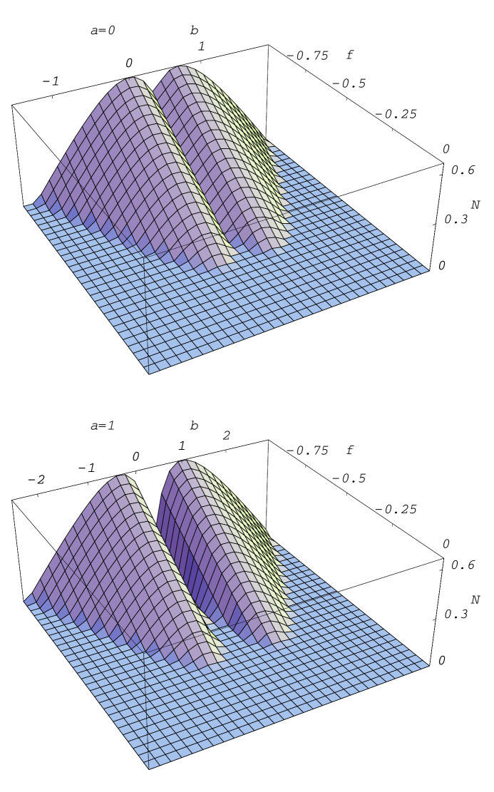
Figure 1: Depiction of $N=\max\{||\widetilde{\rho_{AB}}^{\mathcal{T}_{\{c_{A},r_{B}\}}}||-h_{a}h_{b},0\}$ for a $3\times 3$ Werner state as a function of $b$ and $f$ when $a=0$ (the top figure) and $a=1$ (the bottom figure), respectively.

For the case $a=0$, we see that $N>0$ for all $-1\leq f<-\frac{1}{3}$ and $b=0$ or $\frac{2}{3}$. From the Theorem, we have $h_{a}h_{b}=1$ for $b=0$ or $\frac{2}{3}$ when $a=0$. $\widetilde{\rho_{AB}}$ is in fact the same for $b=0$ or $\frac{2}{3}$ and we obtain $N=\max\{\frac{|1-3f|-2}{3},0\}$ by direct computation. For that case $a=1$, we still have $N>0$ for all $-1\leq f<-\frac{1}{3}$ but with $b=-\frac{1}{3}$ or $1$. Also we see that $h_{a}h_{b}=2$ for $b=-\frac{1}{3}$ or $1$ when $a=1$. $\widetilde{\rho_{AB}}$ is the same for both $b=-\frac{1}{3}$ and $1$. In this case we have again $N=\max\{\frac{|1-3f|-2}{3},0\}$ by direct verification.

Example 2: Horodecki $3\times 3$ bound entangled state

Horodecki gives a very interesting weakly entangled state in hPLA97 which cannot be detected by the $PPT$ criterion. The density matrix $\rho$ is real and symmetric:

$$\rho={\frac{1}{8c+1}}\left[\begin{array}[]{ccccccccc}c&0&0&0&c&0&0&0&c\\ 0&c&0&0&0&0&0&0&0\\ 0&0&c&0&0&0&0&0&0\\ 0&0&0&c&0&0&0&0&0\\ c&0&0&0&c&0&0&0&c\\ 0&0&0&0&0&c&0&0&0\\ 0&0&0&0&0&0&{\frac{1+c}{2}}&0&{\frac{\sqrt{1-c^{2}}}{2}}\\ 0&0&0&0&0&0&0&c&0\\ c&0&0&0&c&0&{\frac{\sqrt{1-c^{2}}}{2}}&0&{\frac{1+c}{2}}\end{array}\right],$$ (33)

where $0<c<1$. The entanglement in this state is very difficult to detect with previous operational criterion in general. In hPLA97 , Horodecki showed that the range criterion could recognize the entanglement. For this state, the simple realignment criterion and its generalization: the GPT criterion can, surprisingly, detect the entanglement for all permissable $c$, as shown in ChenQIC03 . Here, we will observe the behavior in the language of the generalized reduction criterion (for real values of $a$ and $b$, as in Example $1$). The partial transposition $\widetilde{\rho_{AB}}^{\mathcal{T}_{\{r_{A},c_{A}\}}}$ using our Theorem fails to detect the entanglement by direct calculation. Therefore we are only concerned with the case of $\widetilde{\rho_{AB}}^{\mathcal{T}_{\{c_{A},r_{B}\}}}$ which corresponds to the realignment of $\widetilde{\rho_{AB}}$. For the case of $a=0$ and $a=1$, respectively, we plot $N=\max\{||\widetilde{\rho_{AB}}^{\mathcal{T}_{\{c_{A},r_{B}\}}}||-h_{a}h_{b},0\}$ as a function of $b$ and $c$ in Fig.2.

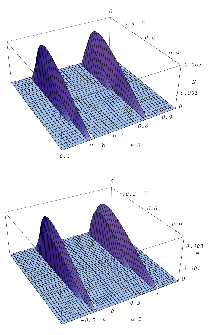
Figure 2: Depiction of $N=\max\{||\widetilde{\rho_{AB}}^{\mathcal{T}_{\{c_{A},r_{B}\}}}||-h_{a}h_{b},0\}$ for a Horodecki $3\times 3$ bound entangled state as a function of $b$ and $c$ when $a=0$ (the top figure) and $a=1$ (the bottom figure), respectively.

For the case of $a=0$, we see that $N>0$ for all $0<c<1$ and $b=0$ or $\frac{2}{3}$. In this case $h_{a}h_{b}=1$ for $b=0$ or $\frac{2}{3}$ when $a=0$. But $\widetilde{\rho_{AB}}$ has different forms for $b=0$ and $\frac{2}{3}$. For the case $a=1$ we still have $N>0$ for all $0<c<1$ but with $b=-\frac{1}{3}$ or $1$. Also we see that $h_{a}h_{b}=2$ and $\widetilde{\rho_{AB}}$ has quite different forms for $b=-\frac{1}{3}$ and $1$ when $a=1$. However, the function $N$ has the same value for the case $a=0$ when $b=0$ or $\frac{2}{3}$, or the case $a=1$ when $b=-\frac{1}{3}$ or $1$.

The results of the above two examples are a little bit surprising compared with the relationship between the PPT and reduction criteria. As is well known, the $PPT$ criterion is equivalent to the reduction criterion for a $2\times n$ system. That is to say, for $a=0$ and $b=1$, or $a=1$ and $b=0$ they give the same result for a $2\times n$ system. But in the case of the $3\times 3$ system, we have identical results for different $b$ other than the value of $0,1$ if we apply the realignment operations to $\widetilde{\rho_{AB}}$. This interesting phenomenon also occurs in higher dimensional cases. So our generalized reduction includes all the results from the original realignment or $GPT$ criteria but recognizes entanglement in a very subtle way which is quite different from other criteria.

IV Conclusion

Summarizing, we have introduced a computational criterion, which we call the “generalized reduction criterion”, providing a necessary condition for separability of bipartite quantum systems in arbitrary dimensions . This criterion combines many virtues of the reduction criterion and the GPT criterion. It gives a unified framework for the two criteria and provides a powerful necessary condition for separability using just simple matrix operations. Some interesting characters of this criterion are showed by two typical examples. The theorem can be straightforwardly generalized to the multipartite case by introducing more free parameters like $a$ and $b$ in the theorem.

We expect that this construction not only expands theoretically our sight in detecting entanglement of a general quantum state, but also sheds some light on possible ways to the final solution of the separability problem. We conjecture that any future stronger operational separability test should in principle include as special cases the simple GPT criterion, in particular the PPT criterion which is necessary and sufficient one for $2\times 2$ and $2\times 3$ system. This paper is an attempt following this way, though we have not yet found an example of a bound entangled state which can be detected by this criterion but not by the GPT criterion.

References

- (1) A. Einstein, B. Podolsky and N. Rosen, Phys. Rev. 47, 777 (1935).
- (2) E. Schrödinger, Natürwissenschaften 23, 807 (1935).
- (3) J.S. Bell, Physics (N.Y.) 1, 195 (1964).
- (4) J. Preskill, The Theory of Quantum Information and Quantum Computation, California Inst. of Tech., 2000, http://www.theory.caltech.edu/people/preskill/ph229/.
- (5) M.A. Nielsen and I.L. Chuang, Quantum Computation and Quantum Information, Cambridge University Press, Cambridge, 2000.
- (6) D. Bouwmeester, A. Ekert and A. Zeilinger (Eds.), The Physics of Quantum Information: Quantum Cryptography, Quantum Teleportation and Quantum Computation, Springer, New York, 2000.
- (7) R.F. Werner, Phys. Rev. A 40, 4277 (1989).
- (8) M. Horodecki, P. Horodecki and R. Horodecki, Springer Tracts in Mod. Phy. 173, 151 (2001).
- (9) M. Lewenstein, D. Bruss, J.I. Cirac, B. Kraus, M. Kus, J. Samsonowicz, A. Sanpera and R. Tarrach, J. Mod. Opt. 47, 2841 (2000).
- (10) B.M. Terhal, Theor. Comput. Sci. 287, 313 (2002).
- (11) A. Peres, Phys. Rev. Lett. 77, 1413 (1996).
- (12) M. Horodecki, P. Horodecki and R. Horodecki, Phys. Lett. A 223, 1 (1996).
- (13) C.H. Bennett, D.P. DiVincenzo, J.A. Smolin and W.K. Wootters, Phys. Rev. A 54, 3824 (1996).
- (14) W.K. Wootters, Phys. Rev. Lett. 80, 2245 (1998).
- (15) M. Horodecki and P. Horodecki, Phys. Rev. A 59, 4206 (1999).
- (16) N.J. Cerf, C. Adami and R.M. Gingrich, Phys. Rev. A 60, 898 (1999).
- (17) A.O. Pittenger and M.H. Rubin, Phys. Rev. A 62, 032313 (2000).
- (18) M.A. Nielsen and J. Kempe, Phys. Rev. Lett. 86, 5184 (2001).
- (19) B. Terhal, Phys. Lett. A 271, 319 (2000).
- (20) M. Lewenstein, B. Kraus, J.I. Cirac and P. Horodecki, Phys. Rev. A 62, 052310 (2000).
- (21) P. Horodecki, M. Lewenstein, G. Vidal and I. Cirac, Phys. Rev. A 62, 032310 (2000).
- (22) S. Albeverio, S.M. Fei and D. Goswami, Phys. Lett. A 286, 91 (2001).
- (23) S.M. Fei, X.H. Gao, X.H. Wang, Z.X. Wang and K. Wu, Phys. Lett. A 300, 555 (2002).
- (24) S.J. Wu, X.M. Chen and Y.D. Zhang, Phys. Lett. A 275, 244 (2000).
- (25) P.X. Chen, L.M. Liang, C.Z. Li and M.Q. Huang, Phys. Rev. A 63, 052306 (2001).
- (26) A.C. Doherty, P.A. Parrilo and F.M. Spedalieri, Phys. Rev. Lett. 88, 187904 (2002).
- (27) O. Rudolph, quant-ph/0202121.
- (28) K. Chen and L.A. Wu, Quant. Inf. Comput. 3, 193 (2003).
- (29) M. Horodecki, P. Horodecki and R. Horodecki, quant-ph/0206008.
- (30) K. Chen and L.A. Wu, Phys. Lett. A 306, 14 (2002).
- (31) O. Rudolph, Physical Review A 67, 032312 (2003).
- (32) N.P. Pitsianis, Ph.D. thesis, The Kronecker Product in Approximation and Fast Transform Generation Cornell University, New York, 1997.
- (33) C.F. Van Loan and N.P. Pitsianis, in: Linear Algebra for Large Scale and Real Time Applications, M.S. Moonen and G.H. Golub (Eds.), Kluwer Publications, 1993, pp. 293–314.
- (34) R.A. Horn and C.R. Johnson, Matrix Analysis, Cambridge University Press, New York, 1985.
- (35) R.A. Horn and C.R. Johnson, Topics in Matrix Analysis, Cambridge University Press, New York, 1991.
- (36) P. Horodecki, Phys. Lett. A 232, 333 (1997).