Decoherence of electron beams by electromagnetic field fluctuations

Abstract

Electromagnetic field fluctuations are responsible for the destruction of electron coherence (dephasing) in solids and in vacuum electron beam interference. The vacuum fluctuations are modified by conductors and dielectrics, as in the Casimir effect, and hence, bodies in the vicinity of the beams can influence the beam coherence. We calculate the quenching of interference of two beams moving in vacuum parallel to a thick plate with permittivity $\epsilon(\omega)=\epsilon_{0}+i4\pi\sigma/\omega$. In case of an ideal conductor or dielectric $(|\epsilon|=\infty)$ the dephasing is suppressed when the beams are close to the surface of the plate, because the random tangential electric field $E_{t}$, responsible for dephasing, is zero at the surface. The situation is changed dramatically when $\epsilon_{0}$ or $\sigma$ are finite. In this case there exists a layer near the surface, where the fluctuations of $E_{t}$ are strong due to evanescent near fields. The thickness of this near - field layer is of the order of the wavelength in the dielectric or the skin depth in the conductor, corresponding to a frequency which is the inverse electron time of flight from the emitter to the detector. When the beams are within this layer their dephasing is enhanced and for slow enough electrons can be even stronger than far from the surface.

1 Introduction

Quantum electromagnetic (EM) field fluctuations are well known as being responsible for the Casimir forces, see for example [1]. Less known is the role of these fluctuations in destructing electron coherence. In weak localization phenomena in solids EM fluctuations are one of the dephasing mechanisms of conduction electrons [2], see also [3]. The interference of vacuum electron beams, observed experimentally [4, 5], is also quenched by EM fluctuations [6], see also [7]. These two papers consider EM fluctuations in vacuum or when ideal conductors are present in the vicinity of the beams. The role of dissipation was discussed in Ref. [8]. Based on physical arguments, the decoherence was related to the deceleration of an electron from the beam due to the Ohmic dissipation of the current produced in the metal by the image charge.

The aim of this paper is to extend the calculations of Refs. [6, 7] to the case where the beams are close to dissipative bodies and to consider in detail the experiment geometry when two interfering beams move in vacuum parallel to a thick infinite plate with permittivity $\epsilon(\omega)=\epsilon_{0}+i\;4\pi\sigma/\omega$. Calculations of the dephasing factor in this geometry demonstrate the crucial role of dissipation. If the plate is an ideal conductor, $\sigma=\infty$, the fluctuations of the tangential electric field $E_{t}$, which are responsible for beam dephasing in this geometry, are suppressed near the plate surface because of the boundary condition $E_{t}=0$ at the surface. However, when $\sigma$ is finite, very strong fluctuations of $E_{t}$ exist near the plate surface, within a layer of the order of the skin depth. These near-field fluctuations dramatically enhance the beam dephasing. Unexpectedly, a similar effect exists also near a lossless dielectric with high permittivity, $\sigma=0,\epsilon_{0}\gg 1$, within a layer of the order of the wave length in the dielectric.

The paper is organized as follows. In Sec.2 we present the dephasing factor $e^{-K}$ in terms of the EM field correlator ${\cal D}$ in the case of no dissipation, Eq.(7), and give reasons why the quantum Langevin equation for the EM field has to be used when dissipation is present. In Sec.3 we derive the Langevin equation and prove that the expression of $K$ in terms of ${\cal D}$ is valid in the case of dissipation too. In this section we present also the relation between ${\cal D}$ and the EM field retarded Green function ${\cal G}$, which is used to calculate ${\cal D}$. The above mentioned special geometry is considered in Sec.4, where $K$ is given as an integral, Eq.(32), over wave vectors and frequencies, containing the spectral density of the EM field fluctuations $\langle E_{t}E_{t}\rangle_{{\bf k}\omega}$, and the spectral density $|({\bf l})_{{\bf k}\omega}|^{2}$ of the EM field radiated by the beam electrons. $\langle E_{t}E_{t}\rangle_{{\bf k}\omega}$ is calculated in Sec.5 and Sec.6, where Eqs.(53) and (54) demonstrate the enhancement of fluctuations due to near fields. In Sec.7 we present a model for $|({\bf l})_{{\bf k}\omega}|^{2}$ and calculate explicitly $K$ as a function of the distance of the beams from the plate $d$ and the electron velocity $v$ (see Eqs.(61),(62) and (63) and the text which follows). It turns out that the dephasing enhancement due to near fields is appreciable when $v$ and $\sigma$ are not very large. In Sec.8 we discuss the relation between beam dephasing and beam EM radiation. The Appendix contains some calculation details.

2 Beam dephasing

If one ignores the interaction of the beam electrons with the EM field, the number of electrons measured in the interference experiment is $n=|\psi_{1}|^{2}+|\psi_{2}|^{2}+2{\rm Re}(\psi_{1}\psi_{2}^{*}),$ where $\psi_{1}$ and $\psi_{2}$ are the wave-functions corresponding to the coherent motion of the electrons in beams 1 and 2, and $n$ is calculated at the detector position. The interaction with the EM field does not affect the squares $|\psi_{1}|^{2}$ and $|\psi_{2}|^{2}$ (since it does not change the number of electrons in the beams), but the product $\psi_{1}\psi_{2}^{*}$, responsible for the interference pattern, is multiplied by a factor $e^{i\phi}e^{-K}$ with real $\phi$ and positive $K$. The first factor only shifts the interference pattern in space, while the second one reduces the amplitude of the interference oscillations (compared to the background $|\psi_{1}|^{2}+|\psi_{2}|^{2}$) and describes dephasing.

To calculate the strength of dephasing we use the ”trace of the environment” picture [3]. At $t=t_{0}$, when the electron is emitted from the source, the environment is in state $|t_{0}\rangle$. While moving, the electron interacts with the environment and perturbs its state. When the electron moving in beam 1 arrives the detector at time $t_{1}$, the environment evolves due to this interaction to state $|t_{1}\rangle$. In a similar way one defines the state $|t_{2}\rangle$. According to the ”trace of the environment” picture $e^{i\phi}e^{-K}=\langle t_{2}|t_{1}\rangle.$

One can present the final states of the environment in terms of evolution operators,

$$|t_{1}\rangle=U_{1}|t_{0}\rangle,\qquad U_{1}={\cal T}\exp\left[-\frac{i}{\hbar}\int_{t_{0}}^{t_{1}}dtH_{1}(t)\right],$$ (1)

where ${\cal T}$ means time ordering and $H_{1}(t)$ is the interaction of the electron in beam 1 with the environment. $H_{1}(t)$ is in the interaction representation, i.e. sandwiched with evolution exponents $\exp[-i{\cal H}t/\hbar]$ containing the beam electron Hamiltonian and the environment Hamiltonian. In a similar way one defines $U_{2}$ in terms of $H_{2}(t)$ and finds $\langle t_{2}|t_{1}\rangle=\langle t_{0}|U_{2}^{-1}U_{1}|t_{0}\rangle.$ For an EM environment, choosing a gauge with zero scalar potential, we have

$$H_{1}(t)=-\frac{1}{c}\int d{\bf r}\,{\bf j}_{1}({\bf r},t){\bf A}({\bf r},t),$$ (2)

where ${\bf j}_{1}$ electron current density operator for the electron in beam 1 (sandwiched with the evolution exponents containing the beam electron Hamiltonian) and ${\bf A}$ the vector potential operator (sandwiched with the evolution exponents containing the EM environment Hamiltonian). $H_{2}(t)$ is defined similarly with the current ${\bf j}_{2}$.

In this approach one assumes that at the initial moment $t_{0}$ the electron source and the environment are un-correlated. It is also assumed that the renormalization of the bare electron parameters due to the interaction with the EM environment [7] does not influence substantially the dephasing phenomena.

To proceed we assume, following [6], that the current is a classical quantity. When there is no dissipation in the EM environment, its Hamiltonian is simply the EM field Hamiltonian and the EM field can be quantized expanding it in normal modes. It is well known that in this case the commutator $[{\bf A}({\bf r},t),{\bf A}({\bf r}^{\prime},t^{\prime})]$ is an imaginary c-number, and due to the classical nature of the currents ${\bf j}_{1}$ and ${\bf j}_{2}$ the commutators of $H_{1}(t)$ and $H_{2}(t^{\prime})$ have the same property. Because of this property the time ordering affects only the phase of the evolution operators [9], and one can obtain

$$U_{1}=e^{i\phi_{1}}V_{1},\qquad V_{1}=\exp\left[-\frac{i}{\hbar}\int_{-\infty}^{\infty}dtH_{1}(t)\right],$$ (3)

if $H_{1}$ is defined to be zero for $t<t_{0}$ and for $t>t_{1}$. The phase $\phi_{1}$ contains the commutator $[H_{1}(t),H_{1}(t^{\prime})]$. Defining $H_{2}(t)$ in a similar way, we have

$$U_{2}^{-1}U_{1}=e^{i(\phi_{1}-\phi_{2})}V_{2}^{-1}V_{1}=e^{i(\phi_{1}-\phi_{2})}e^{i\chi}\exp\left[-\frac{i}{\hbar}\int_{-\infty}^{\infty}dt(H_{1}(t)-H_{2}(t))\right],$$ (4)

where the additional phase $\chi$ contains the commutator $[H_{1}(t),H_{2}(t^{\prime})]$. Averaging this over $|t_{0}\rangle$ we find

$$\langle t_{2}|t_{1}\rangle = e^{i\phi}e^{-K}=e^{i(\phi_{1}-\phi_{2}+\chi)}\left\langle\exp\left[\frac{i}{\hbar c}\int_{-\infty}^{\infty}dt\int d{\bf r}\;{\bf j}_{12}({\bf r},t){\bf A}({\bf r},t)\right]\right\rangle,$$ (5)

where ${\bf j}_{12}({\bf r},t)={\bf j}_{1}({\bf r},t)-{\bf j}_{2}({\bf r},t)$ and $\langle...\rangle$ means average over $|t_{0}\rangle$. When the initial state of the environment is an equilibrium state with temperature $T$, the average means a thermal average $\langle...\rangle_{T}$.

The second important property of ${\bf A}({\bf r},t)$ in the case of no dissipation is that it is a Gaussian operator with respect to thermal averaging $\langle...\rangle_{T}$. After expanding ${\bf A}$ in normal modes this property follows from the relation [9]

$$\langle\exp(\alpha^{*}a^{\dagger}-\alpha a)\,\rangle_{T} = \exp\left[\frac{1}{2}\langle(\alpha^{*}a^{\dagger}-\alpha a)^{2}\rangle_{T}\right]=\exp\left[-|\alpha|\,^{2}\left(n+\frac{1}{2}\right)\right],$$ (6)

where $a^{\dagger}$ is the bosonic operator creating a photon in some normal mode, $n=\langle a^{\dagger}a\rangle_{T}$ is the occupation number of this mode, and $\alpha$ is a complex number. Using the Gaussian properties of ${\bf A}$ one can perform the thermal averaging in Eq.(5) and obtain

$$K=\frac{1}{2(\hbar c)^{2}}\int dtdt^{\prime}\int d{\bf r}d{\bf r}^{\prime}j_{12}^{\alpha}({\bf r},t)j_{12}^{\beta}({\bf r}^{\prime},t^{\prime})\langle A_{\alpha}({\bf r},t)A_{\beta}({\bf r}^{\prime},t^{\prime})\rangle_{T},$$ (7)

where $\alpha,\beta=x,y,z$. If one defines the thermal correlator

$${\cal D}_{\alpha\beta}({\bf r},{\bf r}^{\prime};t-t^{\prime})=\frac{1}{2}\langle A_{\alpha}({\bf r},t)A_{\beta}({\bf r}^{\prime},t^{\prime})+A_{\beta}({\bf r}^{\prime},t^{\prime})A_{\alpha}({\bf r},t)\rangle_{T},$$ (8)

the final result is

$$K=\frac{1}{2(\hbar c)^{2}}\int dtdt^{\prime}\int d{\bf r}d{\bf r}^{\prime}j_{12}^{\alpha}({\bf r},t)j_{12}^{\beta}({\bf r}^{\prime},t^{\prime}){\cal D}_{\alpha\beta}({\bf r},{\bf r}^{\prime};t-t^{\prime}).$$ (9)

It was obtained for $T=0$ in Ref.[6] and for $T\neq 0$ in Ref.[7]. We derived it in a different way to emphasize the two assumptions under which this result is valid (for classical currents), namely: (i) the commutator of the field operator ${\bf A}({\bf r},t)$ is an imaginary $c$-number and (ii) ${\bf A}({\bf r},t)$ is a Gaussian quantity with respect to thermal averaging.

When dissipation is present, the EM environment Hamiltonian includes not only the EM field, but also the electrons in the absorbing bodies and their interaction with the EM field. If the field operator ${\bf A}$ is defined as sandwiched by evolution exponents containing the EM field Hamiltonian only, it has to be considered as a random quantity due to the influence of the dissipative electron system in the absorbing bodies. These electrons are the thermal bath, whose temperature defines the temperature of the EM field. Being a random operator, ${\bf A}$ obeys the quantum Langevin equation, where the effect of the dissipative electrons is simulated by a random force. We will show in what follows that the crucial properties of ${\bf A}({\bf r},t)$ used to derive Eq.(9) are valid also for the random vector potential operator, and hence Eq.(9) is valid when dissipative bodies are present. Note, that in case of dissipation normal modes of the EM field do not exist, the EM field can not be quantized in the usual way, and this is why one is forced to use the Langevin equation approach.

3 Quantum Langevin equation for the EM field

A quantum Langevin equation for the coordinate operator $q$ of a particle moving in potential $V(q)$, derived in Ref. [10], can be written in terms of the particle Lagrangian $L=m\dot{q}^{2}/2+V(q)$ as

$$\frac{d}{dt}\frac{\partial L}{\partial\dot{q}(t)}-\frac{\partial L}{\partial q(t)}+\int_{-\infty}^{t}dt^{\prime}\gamma(t-t^{\prime})\dot{q}(t^{\prime})=F(t).$$ (10)

The kernel $\gamma$ is responsible for the ”friction” produced by the environment, which is a thermal bath at temperature $T$, and the operator $F(t)$ is the random force. The statistical and commutation properties of the random force are defined by the dissipation kernel $\gamma$. Namely, $F(t)$ is a Gaussian stationary random process with $\langle F\rangle=0$ and a correlator

$$\frac{1}{2}\left\langle F(t)F(t^{\prime})+F(t^{\prime})F(t)\right\rangle=\frac{1}{2\pi}\int_{-\infty}^{\infty}d\omega\;\exp[-i\omega(t-t^{\prime})]\hbar\omega\coth\frac{\hbar\omega}{2T}\,{\rm Re}\gamma(\omega),$$ (11)

while the commutator of the random force is an imaginary $c$-number,

$$[F(t),F(t^{\prime})]=\frac{2}{\pi}\int_{-\infty}^{\infty}d\omega\exp[-i\omega(t-t^{\prime})]\;\hbar\omega\,{\rm Re}\gamma(\omega).$$ (12)

(Note, that this Langevin equation is equivalent to the well-known approaches used by Feynman and Vernon [11] and Caldeira and Legget [12]).

Consider the classical Maxwell equations for the long-wave EM field, ${\rm rot}{\bf E}=-\dot{{\bf H}}/c$ and ${\rm rot}{\bf H}=\dot{{\bf D}}/c+(4\pi/c){\bf j}$, where ${\bf D}$ is the displacement given by

$${\bf D}({\bf r},t)={\bf E}({\bf r},t)+\int_{-\infty}^{t}dt^{\prime}\;\chi({\bf r},t-t^{\prime}){\bf E}({\bf r},t^{\prime}),$$ (13)

and ${\bf j}$ is the external current density. Note that fields entering the above macroscopic equations are averaged over a volume $\Delta V=(\Delta L)^{3}$, where $\Delta L$ is large compared to all relevant microscopic lengths, but small compared to the wave-length of the EM field. With the gauge ${\bf E}=-\dot{{\bf A}}/c$ and ${\bf H}={\rm rot}{\bf A}$ the first Maxwell equation is satisfied and the second gives an equation for the vector potential

$$\frac{1}{c^{2}}\ddot{{\bf A}}(t) + {\rm rot}{\rm rot}{\bf A}(t)+\frac{1}{c^{2}}\int dt^{\prime}\dot{{\bf A}}(t^{\prime})\dot{\chi}(t-t^{\prime})=\frac{4\pi}{c}{\bf j}(t).$$ (14)

Starting from the EM field Lagrangian one can prove that this equation can be considered as the quantum Langevin equation for the random field operator ${\bf A}$, if ${\bf j}$ is the appropriate random force created by the thermal bath of dissipative electrons. ($j_{\alpha}\Delta V/c$ plays the role of $F$ and $\dot{\chi}\Delta V/4\pi c^{2}$ plays the role of $\gamma$.) The correlator of this force is known from the fluctuation-dissipation theorem [13],

$$\frac{1}{2}\left\langle j_{\alpha}({\bf r},t)j_{\beta}({\bf r}^{\prime},t^{\prime})+j_{\beta}({\bf r}^{\prime},t^{\prime})j_{\alpha}({\bf r},t)\right\rangle=\int d\omega\;e^{-i\omega(t-t^{\prime})}(j_{\alpha}({\bf r})j_{\beta}({\bf r}^{\prime}))_{\omega}$$ (15)

with

$$(j_{\alpha}({\bf r})j_{\beta}({\bf r}^{\prime}))_{\omega}=\delta_{\alpha\beta}\delta({\bf r}-{\bf r}^{\prime})\frac{\hbar}{8\pi^{2}}\;\omega^{2}\coth\frac{\hbar\omega}{2T}\;{\rm Im}\epsilon({\bf r},\omega).$$ (16)

Comparing this correlator with Eq.(11), we can find from Eq.(12) the commutator of the random currents, which turns out to be an imaginary $c$-number,

$$[j_{\alpha}({\bf r},t),j_{\beta}({\bf r}^{\prime},t^{\prime})]=\delta_{\alpha\beta}\delta({\bf r}-{\bf r}^{\prime})\frac{\hbar}{2\pi^{2}}\int d\omega e^{-i\omega(t-t^{\prime})}\omega^{2}\;{\rm Im}\epsilon({\bf r},\omega).$$ (17)

(The quantum Langevin equation for the EM field was considered also in Ref.[14], but in a form not suitable for our problem.)

The retarded Green function, corresponding to Eq.(14), obeys

$$\frac{1}{c^{2}}\ddot{{\cal G}}_{\alpha\lambda}({\bf r},{\bf r}^{\prime};t)+{\rm rot}{\rm rot}_{\alpha\beta}{\cal G}_{\beta\lambda}({\bf r},{\bf r}^{\prime};t)+\frac{1}{c^{2}}\int dt^{\prime}\dot{{\cal G}}_{\alpha\lambda}({\bf r},{\bf r}^{\prime};t^{\prime})\dot{\chi}(t-t^{\prime})$$ (18)

$$=-4\pi\delta_{\alpha\lambda}\delta({\bf r}-{\bf r}^{\prime})\delta(t),$$

with the condition ${\cal G}(t)=0$ for $t<0$. (The ${\rm rot}$ operators are defined in terms of the antisymmetric tensor $\delta_{\alpha\sigma\beta}$ as ${\rm rot}_{\alpha\beta}=\delta_{\alpha\sigma\beta}\nabla_{\sigma}$ and ${\rm rot}{\rm rot}_{\alpha\beta}=\nabla_{\alpha}\nabla_{\beta}-\delta_{\alpha\beta}\nabla^{2}$.) Using this Green function one can calculate the random field operator

$$A_{\alpha}({\bf r},t)=-\frac{1}{c}\int dt^{\prime}\int d{\bf r}^{\prime}{\cal G}_{\alpha\beta}({\bf r},{\bf r}^{\prime};t-t^{\prime})j_{\beta}({\bf r}^{\prime},t^{\prime}).$$ (19)

Two important consequences follows from this relation. First, as the commutator of the currents is an imaginary $c$-number and the ${\cal G}$ is real, the commutator of the random field operators is also an imaginary $c$-number. Second, as the current is a stationary Gaussian process and ${\cal G}$ depends on $t-t^{\prime}$, same is the random field operator. Since these two properties of the field operator were crucial for deriving the dephasing factor as given by Eq.(9) for the case of no dissipation, we proved thereby that this result is valid also when dissipation is present.

The last equation allows also the calculation of the correlator and the commutator of the field operator. The correlator is known [15] to be related to the Green function defined by Eq.(18),

$${\cal D}_{\alpha\beta}({\bf r},t;{\bf r}^{\prime},t^{\prime})=\int d\omega\;e^{-i\omega(t-t^{\prime})}(A_{\alpha}({\bf r})A_{\beta}({\bf r}^{\prime}))_{\omega}$$ (20)

with

$$(A_{\alpha}({\bf r})A_{\beta}({\bf r}^{\prime}))_{\omega}=-\frac{\hbar}{\pi}\coth\frac{\hbar\omega}{2T}\;{\rm Im}{\cal G}_{\alpha\beta}(\omega;{\bf r},{\bf r}^{\prime}),$$ (21)

where the Green function in the frequency domain is defined as

$${\cal G}_{\beta\lambda}({\bf r},{\bf r}^{\prime};t) = \int\frac{d\omega}{2\pi}e^{-i\omega t}{\cal G}_{\beta\lambda}(\omega;{\bf r},{\bf r}^{\prime}).$$ (22)

The definition of ${\cal G}(\omega)$ corresponds to that in [16]. The Green function is symmetric, ${\cal G}_{\beta\lambda}(\omega;{\bf r},{\bf r}^{\prime})={\cal G}_{\lambda\beta}(\omega;{\bf r}^{\prime},{\bf r}),$ and it follows from the properties of $\epsilon({\bf r},\omega)$ that ${\cal G}_{\beta\lambda}(\omega;{\bf r},{\bf r}^{\prime})^{*}={\cal G}_{\beta\lambda}(-\omega;{\bf r},{\bf r}^{\prime}).$ One can prove the following important integral relation

$$\frac{\omega^{2}}{c^{2}}\int d{\bf r}_{0}{\rm Im}\epsilon({\bf r}_{0},\omega){\cal G}_{\lambda\alpha}(\omega;{\bf r},{\bf r}_{0}){\cal G}_{\lambda^{\prime}\alpha}(\omega;{\bf r}^{\prime},{\bf r}_{0})^{*}=-4\pi{\rm Im}{\cal G}_{\lambda\lambda^{\prime}}(\omega;{\bf r},{\bf r}^{\prime}),$$ (23)

which is an obvious generalization to 3D of the 1D relation given in [14]. (It can be proven using the following Green theorem: $\int d{\bf r}\;\phi\;{\rm rot}{\rm rot}_{\alpha\beta}\psi=\int d{\bf r}\;{\rm rot}_{\sigma\alpha}\phi\;{\rm rot}_{\sigma\beta}\psi.$). Using this integral relation one can obtain Eq.(21) and also calculate the commutator

$$[A_{\alpha}({\bf r})_{\omega},A_{\beta}({\bf r}^{\prime})_{\omega^{\prime}}]=-\delta(\omega+\omega^{\prime})\frac{2\hbar}{\pi^{2}}{\rm Im}{\cal G}_{\alpha\beta}(\omega;{\bf r},{\bf r}^{\prime}).$$ (24)

It is important to notice that deriving Eq.(21) and Eq.(24) with the help of Eq.(23) one has to assume that the temperature (entering Eq.(16)) is constant over the whole space (where ${\rm Im}\,\epsilon\neq 0$). This is correct in thermal equilibrium, when all absorbing bodies are at the same temperature, and hence Eq.(21) provides the correlator for the equilibrium EM field. But it does not provide the correlator for the nonequilibrium thermal EM radiation, when there is radiation energy exchange between bodies with different temperatures. This correlator can be also calculated using Eq. (16), but the integral over the source point can not be simplified using Eq.(23).

4 Dephasing by an infinite thick plate

In what follows we consider a simple geometry when the dephasing body is a half-space $z<0$ with $\epsilon({\bf r},\omega)=\epsilon(\omega)$ and the two beams move in vacuum $z>0$ in a plane $z=d$ parallel to the interface. In this geometry the Green function of the EM field is translational invariant in the $x,y$ plane and hence can be presented as follows [16]

$${\cal G}_{\alpha\beta}(\omega;{\bf r},{\bf r}^{\prime})=\int\frac{d^{2}k}{(2\pi)^{2}}\;e^{i{\bf k}({\bf R}-{\bf R}^{\prime})}g_{\alpha\beta}(\omega,{\bf k}|z,z^{\prime}),$$ (25)

where ${\bf R}$ is the component of ${\bf r}$ in the $(x,y)$ plane and ${\bf k}$ is a vector in this plane. Because of the special geometry we are interested in the Green function ${\cal G}$ for $z=z^{\prime}=d$ and $\alpha,\beta=x,y$, and will denote $g_{\alpha\beta}(\omega,{\bf k}|d,d)\equiv g_{\alpha\beta}(\omega,{\bf k})$. Using the explicit expressions for $g_{\alpha\beta}$ given in [16], one can write

$$g_{\alpha\beta}(\omega,{\bf k})=g_{t}(\omega,k)\left[\frac{k_{\alpha}k_{\beta}}{k^{2}}-\frac{1}{2}\delta_{\alpha\beta}\right]+\frac{1}{2}\delta_{\alpha\beta}\;g_{l}(\omega,k),$$ (26)

where

$$g_{l,t}(-\omega,k)=g_{l,t}(\omega,k)^{*},\qquad g_{\alpha\beta}(\omega,-{\bf k})=g_{\alpha\beta}(\omega,{\bf k})=g_{\alpha\beta}(-\omega,{\bf k})^{*}.$$ (27)

The $g_{\alpha\beta}(\omega,{\bf k})$ are related to the correlator of the tangential components of the electric field in the plane $z=d$. Using Eqs.(27) one can check from Eq.(21) that for $\alpha,\beta=x,y$

$$(E_{\alpha}({\bf R})E_{\beta}({\bf R}^{\prime}))_{\omega}=\int d^{2}k\;e^{i{\bf k}({\bf R}-{\bf R}^{\prime})}(E_{\alpha}E_{\beta})_{\omega{\bf k}}$$ (28)

with

$$(E_{\alpha}E_{\beta})_{\omega{\bf k}}=\frac{2\hbar}{(2\pi)^{3}}\left(\frac{\omega}{c}\right)^{2}\coth\frac{\hbar\omega}{2T}\;(-{\rm Im}g_{\alpha\beta}(\omega,{\bf k})).$$ (29)

The classical current in beam 1 is $j_{1}({\bf r},t)=e{\bf v}_{1}(t)\delta({\bf R}-{\bf R}_{1}(t))\delta(z-d),$ where ${\bf R}_{1}(t)$ is the trajectory of beam 1 and ${\bf v}_{1}(t)=d{\bf R}_{1}(t)/dt$ is the electron velocity in this beam. One can present

$${\bf j}_{1}({\bf r},t)=e\delta(z-d)\int\frac{d^{2}k}{(2\pi)^{2}}\int d\omega\;e^{-i\omega t+i{\bf k}{\bf R}}\;({\bf l}_{1})_{{\bf k}\omega},$$ (30)

where the radiation amplitude is

$$({\bf l}_{1})_{{\bf k}\omega}=\int\frac{dt}{2\pi}{\bf v}_{1}(t)\;e^{i\omega t-i{\bf k}{\bf R}_{1}(t)}.$$ (31)

The relevant frequencies and wave vectors are those of the EM field created by the electron in beam 1. Similar expressions can be written for beam 2. We now introduce into the dephasing integral, Eq.(9), the correlator ${\cal D}$ expressed in terms of ${\cal G}$ according to Eq.(20), and the Fourier expansions of ${\bf j}_{1,2}$ and ${\cal G}$ according to Eq.(30) and Eq.(25), we find, using Eqs.(27),

$$K=\frac{e^{2}}{2\hbar c^{2}}\int_{0}^{\infty}\frac{d\omega}{2\pi}\coth\frac{\hbar\omega}{2T}\int\frac{d^{2}k}{(2\pi)^{2}}\left\{-{\rm Im}g_{\alpha\beta}(\omega,{\bf k})\right\}\;[(l_{\alpha})^{*}_{{\bf k}\omega}(l_{\beta})_{{\bf k}\omega}+c.c.],$$ (32)

where $({\bf l})_{{\bf k}\omega}=({\bf l}_{1})_{{\bf k}\omega}-({\bf l}_{2})_{{\bf k}\omega}$. The contribution to this integral comes from frequencies and wave vectors which are present simultaneously in the fluctuation spectra $g(\omega,{\bf k}$) and the radiation spectra $({\bf l})_{{\bf k}\omega}$. Using Eq.(26) one can rewrite the integral over $d^{2}k$ as follows

$$\frac{1}{2\pi}\int_{0}^{\infty}dkk\left\{-2{\rm Im}g_{t}(\omega,k)\langle|\hat{l}_{{\bf k}\omega}|^{2}\rangle-{\rm Im}[g_{l}(\omega,k)-g_{t}(\omega,k)]\langle|({\bf l})_{{\bf k}\omega}|^{2}\rangle\right\},$$ (33)

where $\langle...\rangle$ means angular average and $\hat{l}_{{\bf k}\omega}={\bf k}({\bf l})_{{\bf k}\omega}/k$.

For slow enough electrons one can use the dipole approximation (DA), when the term ${\bf k}{\bf R}_{1}(t)$ in Eq.(31) can be neglected. The condition for this is $\omega\gg kv$, where $\omega$ and $k$ are the typical frequency and wave vector of the EM fluctuations contributing to the integral $K$, and $v$ is the characteristic electron velocity. In this approximation $({\bf l}_{1})_{{\bf k}\omega}\equiv({\bf l}_{1})_{\omega}$, and $e({\bf l}_{1})_{\omega}$ is the radiating dipole moment. Now $({\bf l})_{{\bf k}\omega}=({\bf l}_{1})_{\omega}-({\bf l}_{2})_{\omega}\equiv({\bf l})_{\omega}$. We substitute $({\bf l})_{\omega}$ into Eq.(32) and as a result in the DA the dephasing integral is

$$K=\frac{e^{2}}{2\hbar c^{2}}\int_{0}^{\infty}\frac{d\omega}{2\pi}\coth\frac{\hbar\omega}{2T}\;S(\omega)\;|({\bf l})_{\omega}|^{2},$$ (34)

where

$$|({\bf l})_{\omega}|^{2}=|(l_{x})_{\omega}|^{2}+|(l_{y})_{\omega}|^{2},\qquad S(\omega)=-{\rm Im}\int\frac{d^{2}k}{(2\pi)^{2}}g_{l}(\omega,k).$$ (35)

$S(\omega)$ is related to average amplitude of the tangential electric field at distance $d$ from the interface. From Eq.(28) at ${\bf R}^{\prime}={\bf R}$ one finds

$$(E^{2}_{t})_{\omega}=(E^{2}_{x}+E^{2}_{y})_{\omega}=\frac{\hbar}{\pi}\left(\frac{\omega}{c}\right)^{2}\coth\frac{\hbar\omega}{2T}\;S(\omega).$$ (36)

It is convenient to represent $K=K_{p}+K_{e}$, where the two terms are the contributions to the integral of the domains, correspondingly, $k<\omega/c$ and $k>\omega/c$. In the first domain the wave vector component perpendicular to the interface $k_{z}=\sqrt{(\omega/c)^{2}-k^{2}}$ is real, which means that this domain corresponds to waves propagating perpendicular to the interface (PW), while in the second one $k_{z}$ is imaginary and it corresponds to evanescent waves (EW).

5 Spectral densities $g(\omega,k)$

Using the explicit expressions for $g_{\alpha\beta}$ given in [16], one can find (for $\omega>0$)

$$g_{l,t}(\omega,k)=\frac{2\pi i}{k_{0}}[e^{ipu(\xi)}F_{l,t}(\xi)-G_{l,t}(\xi)],$$ (37)

where $\xi=|{\bf k}|/k_{0}$ with $k_{0}=\omega/c$, and

$$G_{l,t}(\xi)=u\pm\frac{1}{u},\qquad F_{l,t}(\xi)=\pm\frac{1}{u}\;\frac{v-u}{v+u}-u\;\frac{v-\epsilon(\omega)u}{v+\epsilon(\omega)u},$$ (38)

with $u=[1-\xi^{2}]^{1/2},\;v=[\epsilon(\omega)-\xi^{2}]^{1/2},{\rm Im}u>0,\;{\rm Im}v>0$ and $p=2k_{0}d$. The upper sign corresponds to $l$ and the lower to $t$.

Consider the spectral densities $(-{\rm Im}g_{l,t})$ in the $(\omega,k)$ plane at $\omega>0,k>0$ (see Figure 1). One important borderline in this plane is $\xi=1$, i.e. $k=\omega/c$, which, as noted above, separates the propagating waves (PW) domain below it from the evanescent waves (EW) domain above it. In the PW domain $\xi<1$ and

$$-{\rm Im}g_{l,t}(\omega,k)=\frac{2\pi}{k_{0}}[G_{l,t}(\xi)-{\rm Re}F_{l,t}(\xi)\cos pu(\xi)],$$ (39)

while in the EW domain $\xi>1$ and

$$-{\rm Im}g_{l,t}(\omega,k)=-\frac{2\pi}{k_{0}}e^{-p\sqrt{\xi^{2}-1}}{\rm Re}F_{l,t}(\xi).$$ (40)

For $\epsilon(\omega)\equiv 1$ one finds $u=v$ and $F(\xi)=0$. This corresponds to empty space, in which case the spectral densities $-{\rm Im}g_{l,t}(\omega,k)\neq 0$ only in the PW domain, where in this case

$$-{\rm Im}g_{l,t}(\omega,k)=\frac{2\pi}{k_{0}}G_{l,t}(\xi).$$ (41)

The same result is obviously obtained far from the interface, when $d\rightarrow\infty$, since one can neglect the oscillating or decaying term in Eq.(37).

The second important borderline is $\xi=|\epsilon(\omega)|^{1/2}$. For a non-dispersive lossless dielectric, ${\rm Im}\epsilon=0,\;\epsilon\equiv n^{2}>1$, this borderline is simply $k=\omega/c_{n}$, where $c_{n}\equiv c/n$ is the light velocity in the dielectric. One easily finds that $-{\rm Im}g_{l,t}(\omega,k)=0$ above the second borderline, for $\xi>n$. Below it, for $1<\xi<n$, one has

$${\rm Re}F_{l,t}(\xi)=-\frac{2}{\epsilon-1}(\epsilon-\xi^{2})^{1/2}\left[\frac{\epsilon(\xi^{2}-1)}{(\epsilon+1)\xi^{2}-\epsilon}\pm 1\right].$$ (42)

In the generic case of arbitrary complex $\epsilon(\omega)$ the spectral densities $(-{\rm Im}g_{l,t})$ are non-zero in the whole $(\omega,k)$ plane.

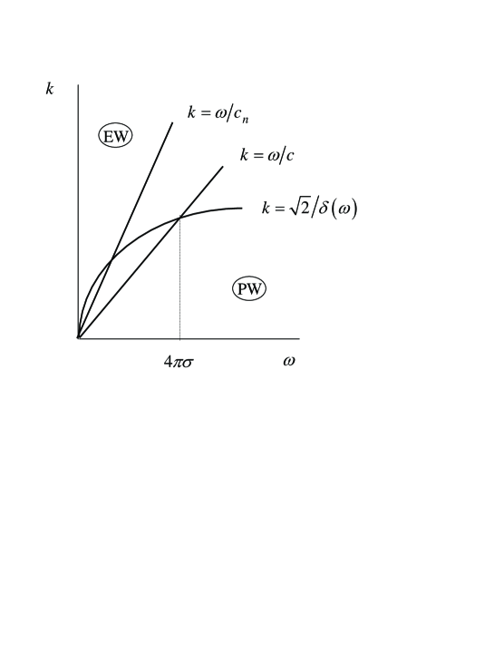
Figure 1: Borderlines in the $(\omega,k)$ plane, see text.

In what follows we will consider two cases: (i) a highly polarizable lossless dielectric, ${\rm Im}\epsilon=0,\;\epsilon\gg 1$, and (ii) a ”good” conductor, ${\rm Im}\epsilon\gg{\rm Re}\,\epsilon\simeq 1$. In the last case we write $\epsilon(\omega)=\epsilon_{0}+i(4\pi\sigma/\omega)$, where $\sigma$ is the conductivity, and assume that $\sigma$ is larger than all relevant frequencies. Both cases correspond to $|\epsilon|\gg 1$ and it is instructive therefore to investigate the limit $|\epsilon|=\infty$. In this limit $F(\xi)=G(\xi)$ and the spectral densities $-{\rm Im}g_{l,t}(\omega,k)\neq 0$ only in the PW domain, where

$$-{\rm Im}g_{l,t}(\omega,k)=\frac{2\pi}{k_{0}}[1-\cos pu(\xi)]G_{l,t}(\xi).$$ (43)

One can see that near the interface with an ideal conductor ($\sigma=\infty$) or an ideal dielectric ($\epsilon_{0}=\infty$) the tangential electric field fluctuations are suppressed. In the case of a conductor it is obvious from the boundary condition $E_{t}=0$. In the case of a dielectric this boundary condition is also effective, since $E_{t}\neq 0$ would mean, due to the continuity of $E_{t}$, infinite energy density in the dielectric or infinite displacement current.

Now we turn to the spectral density corrections which are due to finite $|\epsilon|$. To investigate the role of these corrections we use the following expansions. Well below the second borderline, i.e. at $\xi\ll|\epsilon|^{1/2}$, one has

$$F_{l}(\xi)=G_{l}(\xi)-4\epsilon^{-1/2}+O(\epsilon^{-1}),\qquad F_{t}(\xi)=G_{t}(\xi)\left[1-2\epsilon^{-1}\right]+O(\epsilon^{-3/2}).$$ (44)

Well above the second borderline, i.e. at $\xi\gg|\epsilon|^{1/2}$, one finds

$$F_{l,t}(\xi)=i\;\frac{\epsilon-1}{\epsilon+1}\;\xi+i\left(\frac{\epsilon-1}{\epsilon+1}\right)^{2}\frac{1}{2\xi}+O(\xi^{-3}).$$ (45)

At $\xi\simeq|\epsilon|^{1/2}$ obviously $F_{l,t}(\xi)\simeq|\epsilon|^{1/2}$.

It follows from Eq.(44) that in the PW domain the finite $|\epsilon|$ corrections are small. However as we will see later, these corrections are important in the EW domain at small distances from the interface $d$. To account for these corrections in a dielectric one can use the explicit expressions given by Eq.(42), but for a conductor the situation is more complicated. For a good conductor it is convenient to use the surface impedance $\zeta(\omega)$ and the skin depth $\delta(\omega)$ defined as follows,

$$\zeta(\omega)=(\omega/8\pi\sigma)^{1/2}\approx(2|\epsilon(\omega)|)^{-1/2},\qquad\delta(\omega)=\frac{c}{(2\pi\sigma\omega)^{1/2}}=2\zeta(\omega)\frac{c}{\omega}\;.$$ (46)

In these terms the second borderline is $k=\sqrt{2}/\delta(\omega)$ or $\xi=(\sqrt{2}\zeta(\omega))^{-1}$. Since $\zeta(\omega)\ll 1$ and $\delta(\omega)\ll k_{0}^{-1}$ when $\omega\ll 4\pi\sigma$, this borderline in the EW domain is well above the first borderline $k=\omega/c$.

In between the borderlines, $\omega/c\ll k\ll\delta(\omega)^{-1}$, one can find using Eqs.(44),

$${\rm Re}F_{l}(\xi)=-4\zeta(\omega),\qquad{\rm Re}F_{t}(\xi)=-4\zeta(\omega)^{2}\xi.$$ (47)

Above the upper borderline, $k\gg\delta(\omega)^{-1}$, one finds from Eq.(45), using $(\epsilon-1)/(\epsilon+1)=1+4i\zeta(\omega)^{2}$, the dominant term to be

$${\rm Re}F_{l,t}(\xi)=-4\zeta(\omega)^{2}\xi.$$ (48)

Now we find from Eq.(40) the spectral densities for a good conductor in the EW domain. In between the borderlines

$$-{\rm Im}g_{l}(\omega,k)=\frac{8\pi}{k_{0}}\zeta(\omega)e^{-2kd},\qquad-{\rm Im}g_{t}(\omega,k)=\frac{8\pi}{k_{0}^{2}}\zeta(\omega)^{2}ke^{-2kd},$$ (49)

while above the upper borderline

$$-{\rm Im}g_{l,t}(\omega,k)=\frac{8\pi}{k_{0}^{2}}\zeta(\omega)^{2}ke^{-2kd},\quad-{\rm Im}g_{\alpha\beta}(\omega,k)=\frac{8\pi}{k_{0}^{2}}\zeta(\omega)^{2}ke^{-2kd}\frac{k_{\alpha}k_{\beta}}{k^{2}}.$$ (50)

In the EW domain the fluctuations are small, because of the small surface impedance, and are strongly suppressed at $k\gtrsim d^{-1}$, since random fields created by fluctuations of the random currents with wavelength shorter than $d$ are averaged at distance $d$.

6 Spectral density $S(\omega)$

The spectral density, which enters in the DA, can be split into contributions of the PW and EW domains, $S(\omega)=S_{p}(\omega)+S_{e}(\omega)$, with

$$S_{p}(\omega) = -\frac{1}{2}k_{0}{\rm Re}\int_{0}^{1}d\xi\;\xi[e^{ip\sqrt{1-\xi^{2}}}F_{l}(\xi)-G_{l}(\xi)],$$ (51)

$$S_{e}(\omega) = -\frac{1}{2}k_{0}\int_{1}^{\infty}d\xi\;\xi e^{-p\sqrt{\xi^{2}-1}}{\rm Re}F_{l}(\xi).$$

To avoid misunderstanding we note that the spectral density due to a half-space $z<0$ with $\epsilon(\omega)$ calculated in Ref. [17] is not for the equilibrium EM field, but is for the radiation into a zero temperature half space $z>0$.

In the limit $|\epsilon|=\infty$ only PW contribute and one finds easily the spectral density

$$S(\omega)=S_{p}(\omega)=\frac{\omega}{c}\;\left[\frac{2}{3}-\frac{\cos p}{p^{2}}-\frac{\sin p}{p}\left(1-\frac{1}{p^{2}}\right)\right].$$ (52)

At large distances from the interface, $d\gg k_{0}^{-1}$, one has $S(\omega)=(2/3)k_{0}$, which correspond to EM field fluctuations in empty space. (The factor 2/3 appear because only two tangential components of the electric field are relevant). At small distances, $d\ll k_{0}^{-1}$, the fluctuations are suppressed, $S(\omega)\sim d^{2}$. For an ideal conductor or ideal dielectric the contribution to $S(\omega)$ comes from $\xi\simeq 1$ (i.e. $k\simeq\omega/c$) independent of the value of the parameter $p=2k_{0}d$.

Now we turn to the finite $|\epsilon|$ corrections. One can see from Eq.(44) that the corrections to $S_{p}(\omega)$ are small, and one can use for $S_{p}(\omega)$ the result given by Eq.(52). But this is not the case for $S_{e}(\omega)$ when $d$ is small and the decay of the exponent is this integral is slow. For a dielectric, $S_{e}(\omega)$ can be calculated using Eq.(42) and when $\epsilon=n^{2}\gg 1$ the result is

$$d\ll\lambda_{n}:\quad S_{e}(\omega)=\frac{2}{3}k_{0}n\;;\qquad d\gg\lambda_{n} : \quad S_{e}(\omega)=\frac{1}{2k_{0}n}\,\frac{1}{d^{2}},$$ (53)

where $\lambda_{n}=c_{n}/\omega=(k_{0}n)^{-1}$ is the wave length in the dielectric. The first of Eqs.(53) means simply that the fluctuations of $E_{t}$ at $d\ll\lambda_{n}$ in the vacuum are the same as in the dielectric, which is consistent with the continuity of $E_{t}$ at the interface. Eqs.(53) clearly demonstrate the importance of finite $|\epsilon|$ corrections at small distances. Comparing $S_{e}(\omega)$ for $d\gg\lambda_{n}$ with $S_{p}(\omega)$ from Eq.(52), one can see, that the ideal dielectric approach, when $S(\omega)$ is dominated by PW, is valid only at $d\gg\lambda n^{-1/4}=\lambda_{n}n^{3/4}$, while at smaller distances $S(\omega)$ is dominated by EW. According to the ideal dielectric approximation, Eq.(52), near the interface the fluctuations are suppressed compared to free space, while from the first of Eqs.(53) it follows that they are enhanced compared to free space by a factor $n$. The contribution to the integral $S_{e}(\omega)$ comes from $k\simeq\lambda_{n}^{-1}$, when $d\ll\lambda_{n}$, and from $k\simeq d^{-1}$ when $d\gg\lambda_{n}$. When $S_{e}(\omega)$ dominates, both cases correspond to large imaginary $k_{z}$. In other words, the fluctuations contributing to $S_{e}(\omega)$, are due to near fields localized close to the interface.

The situation in a conductor is different, since from Eq.(48) one can see that the integral $S_{e}(\omega)$ diverges at $d=0$. The near-field fluctuations in the case of a conductor are

$$d\ll\delta(\omega):\;S_{e}(\omega)=\frac{\zeta(\omega)^{2}}{2k_{0}^{2}d^{3}}=\frac{\delta(\omega)^{2}}{8d^{3}};\quad d\gg\delta(\omega):\;S_{e}(\omega)=\frac{\zeta(\omega)}{2k_{0}d^{2}}=\frac{\delta(\omega)}{4d^{2}}.$$ (54)

The near field/far field crossover point is $d_{\times}\simeq(c/\omega)\zeta(\omega)^{1/4}$ and for all $d$ the relevant $k\simeq d^{-1}$. When $d\ll\delta(\omega)$ the relevant $k$ are above the borderline $k=\sqrt{2}/\delta(\omega)$ and the first of Eqs.(54) is obtained using Eq.(50), while when $d\gg\delta(\omega)$ the relevant $k$ are below this borderline and the second of Eqs.(54) is obtained using Eq.(49).

Comparing $S_{e}(\omega)$ for a dielectric and a conductor one can see that they are similar not very close to the interface, if one replaces $n^{-1}$ by $\zeta(\omega)$ and $\lambda_{n}$ by $\delta(\omega)$. The behavior very close to the interface is different, since for a dielectric $S_{e}(\omega)$ is finite, while for a conductor it diverges. (This singularity is cut-off if one takes into account the spatial dispersion of the conductor $\epsilon$ [17]).

7 Dephasing by near fields

To simplify the picture of dephasing we assume that the electrons smoothly accelerate and decelerate. In other words, we assume that the electron motion has only one characteristic time scale $\tau$, which is the time of flight from the emitter to the detector, and only one length scale $L$, which is the trajectory length. The characteristic electron velocity is defined as $v=L/\tau$. We also assume, following the experimental situation, that the beams are close, i.e. the distance between them $a$ is small compared to $L$. The frequencies of the EM waves emitted by the electrons are of the order of $\omega=\tau^{-1}$ and wavelengths are of the order of $\lambda=c\tau$. In this model the angle averages entering the integrals in Eq.(33) and Eq.(34) can be presented as follows:

$$\langle|\hat{l}_{{\bf k}\omega}|^{2}\rangle=\theta L^{2}\Psi_{1}(z,y),\quad\langle|({\bf l})_{{\bf k}\omega}|^{2}\rangle=\theta L^{2}\Psi_{2}(z,y),\quad|({\bf l})_{\omega}|^{2}=\theta L^{2}\Psi_{2}(z,0),$$ (55)

where $z=\omega\tau/2$, $y=kL$, and the small factor $\theta=(a/L)^{2}$ appears because the beams are close and the effective current ${\bf j}_{12}$ is smaller than the beam currents ${\bf j}_{1}$ and ${\bf j}_{2}$. The functions $\Psi$ decay fast enough at $\omega\gtrsim\tau^{-1}$ and $k\gtrsim L^{-1}$, restricting the integration in the $(\omega,k)$ plane in Eq.(32) within the rectangle $\square\equiv[\;0<\omega\lesssim\tau^{-1},\;0<k\lesssim L^{-1}]$, shown in Figure 2 by dashed lines.

The frequency integral in Eq.(34) contains three characteristic frequencies, namely, $T/\hbar$ (the frequency of the EM field thermal fluctuations), $\tau^{-1}$ (the frequency radiated by the electron), and $c/d$ (the frequency which enters the spectral densities $g$). Assuming $v/c=0.1$ and $L=10$ cm, we have $\tau=3\times 10^{-9}$ s. The electro-optical system, which creates, guides and detects the beams, is at room temperature, and this is the temperature of the EM field surrounding the beams. At room temperature $\hbar/T=2.5\times 10^{-14}$ s and obviously always $T/\hbar\gg\tau^{-1}$. Hence one can replace in the integral Eq.(32) $\coth(\hbar\omega/2T)$ by its classical high temperature approximation.

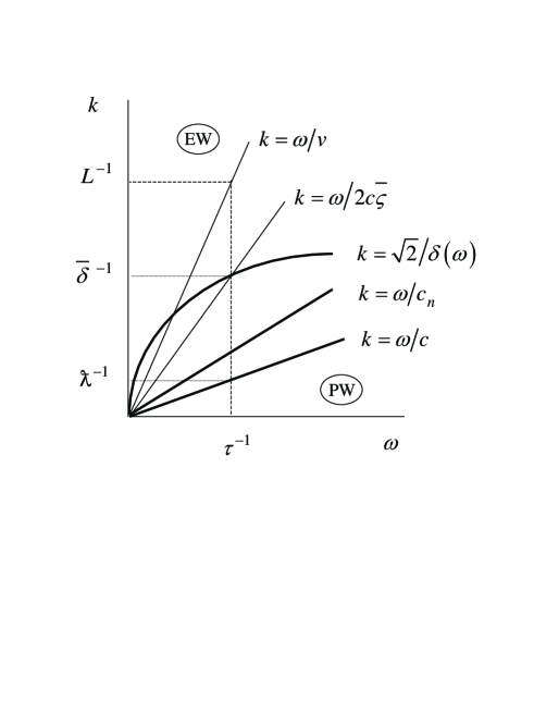
Figure 2: Integration domains in the $(\omega,k)$ plane, see text.

From the spectral densities calculated in sec.5 and sec.6 it follows that when $|\epsilon|\gg 1$ the contribution $K_{p}$ of the PW can be calculated as for an ideal conductor or dielectric. To calculate this contribution one can employ the DA, Eq.(34), because when $|\epsilon|=\infty$ the density $S(\omega)$ comes from $k\simeq\omega/c$, and for non-relativistic electrons the condition for the DA to be valid, namely $kv\ll\omega$, is satisfied.

First we calculate the dephasing near an ideal conductor or ideal dielectric, given by $K_{p}$, Eq.(34). Substituting there $|({\bf l})_{\omega}|^{2}$ from Eq.(55) we obtain

$$d\gg\lambda : \quad K_{p}=K_{0}=b_{p1}\,\alpha\theta\left(\frac{L}{c}\right)^{2}\frac{T/\hbar}{\tau}\;;$$ (56)

$$d\ll\lambda : \quad K_{p}=b_{p2}\,K_{0}\frac{d^{2}}{\lambda^{2}}.$$

Here $K_{0}$ is the dephasing in free space, $\alpha=e^{2}/\hbar c$ is the fine structure constant and the numerical factors $b\simeq 1$ are given in terms of integrals

$$b_{p1}=\frac{2J_{0}}{3\pi},\;b_{p2}=\frac{16J_{2}}{5J_{0}};\quad J_{k}=\int_{0}^{\infty}dzz^{k}\Psi_{2}(z,0).$$ (57)

The second of Eqs.(56) demonstrates that near an ideal conductor and dielectric the dephasing is suppressed. For the parameters used one obtains, neglecting numerical factors, $K_{0}\simeq 10\theta$. This means that for well separated beams $(\theta\simeq 1)$ at room temperature the dephasing due to thermal fluctuations can be significant. In the existing experiments, however, the beams are very close, $a=100\mu$m, and the dephasing is negligible, $K_{0}\simeq 10^{-5}$.

Now we turn to EW contribution $K_{e}$, which is responsible for the enhancement of the dephasing near the interface. As one can see from Figure 2, this contribution is large for small electron velocities $v$, when the overlap of the rectangle $\square$ with the EW domain is maximal. Motivated by this we consider first the simpler case of dielectric for $v\ll c_{n}=c/n$. Since for a dielectric the spectral densities $-{\rm Im}\,g_{l,t}(\omega,k)$ vanish above the borderline $k=\omega/c_{n}$, the integration domain overlaps only with the ”bottom” of the rectangle $\square$, where $k$ is small, meaning that one can employ the DA. Being interested in an almost ideal dielectric ($n\gg 1$), we substitute the spectral density from Eqs.(53) into Eq.(34) and find the dephasing due to near fields to be

$$d\ll\lambda_{n} : \quad K_{e}=\frac{1}{2}K_{0}n;$$ (58)

$$d\gg\lambda_{n} : \quad K_{e}=b_{e}\,K_{0}\frac{\lambda^{2}}{n\,d^{2}},\quad b_{e}=\frac{3J_{-2}}{8J_{0}},$$

where $\lambda_{n}\equiv c\tau/n$. Comparing the second of Eqs.(58) with Eq.(56) one finds the far field - near field crossover for dephasing to be $d_{\times}\simeq\lambda n^{-1/4}$, obviously the same as for $S(\omega)$. Contrary to the predictions of the ideal dielectric approximation $(n=\infty)$ the dephasing of beams moving near the interface is not suppressed compared to empty space, but enhanced by a large factor $n/2$. Since for most dielectrics $n$ does not exceed 10, the condition $v\ll c/n$ is not very severe for non-relativistic electrons, but on the other hand, the enhancement of the dephasing near the interface is not very strong.

The situation is much more complicated for conductors, since the spectral densities $-{\rm Im}\,g_{l,t}(\omega,k)$ do not vanish above the upper borderline $k=\sqrt{2}/\delta(\omega)$ and the integration domain overlaps with the whole rectangle $\square$. The parameter which plays the role of $1/n$ in case of a conductor is $\overline{\zeta}=(8\pi\sigma\tau)^{-1/2}$, i.e. the surface impedance calculated for the characteristic frequency $\tau^{-1}$. Copper at room temperature has $\sigma=5\times 10^{17}$sec${}^{-1}=6\times 10^{5}\,(\Omega{\rm cm})^{-1}$, so for a good conductor this impedance can be as small as $10^{-5}$, and hence the restriction $v\ll\overline{\zeta}c$ can be very severe. As a result one has to consider velocities larger than $\overline{\zeta}c$, when the DA might be invalid. Consequently the calculations are very involved, so we first present the results, discuss them, and sketch the calculations in the Appendix. In what follows we present the results for $\kappa\equiv K/K_{0}$ and the crossover distance $d_{\times}$ from near-field to far-field dephasing. The results are given in terms of the trajectory length $L$, the radiated wave length $\lambda=c\tau$, the surface impedance $\overline{\zeta}$, and the skin depth $\overline{\delta}=2\lambda\overline{\zeta}$. All numerical factors of order one are omitted.

Three velocity intervals are relevant, namely,

$$A:\quad v/c\ll\overline{\zeta};\qquad B:\quad\overline{\zeta}\ll v/c\ll\overline{\zeta}^{1/4};\qquad C:\quad\overline{\zeta}^{1/4}\ll v/c.$$ (59)

The crossover distances from near-field to far-field dephasing in these intervals are as follows

$$A+B:\quad d_{\times}=\overline{\zeta}^{1/4}\lambda;\qquad C:\quad d_{\times}=\overline{\zeta}^{1/2}(\lambda^{2}/L).$$ (60)

The far-field dephasing, at $d\gg d_{\times}$, in all velocity intervals is given by Eq.(56). The near-field dephasing, at $d\ll d_{\times}$, is different in different velocity intervals.
In interval $A$

$$d\ll L:\;\kappa=\overline{\delta}^{2}\lambda/L^{3};\quad L\ll d\ll\overline{\delta}:\;\kappa=\overline{\delta}^{2}\lambda/d^{3};\quad\overline{\delta}\ll d\ll d_{\times}:\;\kappa=\overline{\delta}\lambda/d^{2}.$$ (61)

In interval $B$:

$$d\ll L:\quad\kappa=\overline{\delta}\lambda/L^{2};\qquad L\ll d\ll d_{\times}:\quad\kappa=\overline{\delta}\lambda/d^{2}.$$ (62)

In interval $C$:

$$d\ll d_{\times}:\quad\kappa=\overline{\delta}\lambda/L^{2}.$$ (63)

As one can see from the above results, in the velocity interval $A+B$ the crossover $d_{\times}$ is the same as for $S(\omega)$ and $L\ll d_{\times}\ll\lambda$. In this velocity interval $K$ depends on $d$ in a non-monotonous way, reaching a minimum at $d_{\times}$, where $\kappa\simeq\overline{\zeta}\,^{1/2}$. In the velocity interval $C$ one finds $\overline{\delta}\ll d_{\times}\ll L$ and approaching the interface $K$ decays monotonously till $d\simeq d_{\times}$, where it saturates at $\kappa\simeq\overline{\zeta}(v/c)^{-2}$. For all velocities $K$ is finite at $d=0$, since at very small $d$ the DA is invalid, and the singularity $d^{-3}$ in $S(\omega)$ is cut-off by the ineffectiveness of wave vectors $k\gtrsim L^{-1}$.

As was already mentioned, the dephasing $K_{0}$ in empty space is very weak, and this is why the possible enhancement of $K$ near the interface is of special interest. Looking for the ratio $\eta\equiv K(d=0)/K_{0}$ one can see from the above results that the dephasing near the interface is enhanced compared to that in empty space only for small enough electron velocities, when $v/c\ll\overline{\zeta}\,^{1/2}$, i.e. in the interval $A$ and in the smaller velocity part of interval $B$. Since in the experiment the fixed parameter is not $\tau$, but $L$, and hence $\overline{\zeta}$ depends on $v$, it is more convenient to use a different parameter, namely $\gamma=c/8\pi\sigma L$. In terms of this parameter the velocity interval $A$ is $v/c\ll\gamma$ and the dephasing enhancement in this interval is $\eta=\gamma(v/c)^{-2}$. The smaller velocity part of interval $B$ is $\gamma\ll v/c\ll\gamma\,^{1/3}$ and here $\eta=\gamma\,^{1/2}(v/c)^{-3/2}$. (Note also, that the necessary condition $\overline{\zeta}\ll 1$ reduces to $\gamma(v/c)\ll 1$ and is always satisfied when $\gamma\ll 1$.) For the parameters used above one finds $\gamma\simeq 10^{-10}$ and $\gamma\,^{1/3}\simeq 10^{-3}$. It is clear now that in the case of a good metal the dephasing is enhanced only for relatively slow electrons and is not very high. For example, when $v/c=10^{-4}$ one finds $\eta\simeq 10$. Much stronger dephasing can be achieved with a high resistivity semiconductor, for example Si with $\sigma=1\,(\Omega{\rm cm})^{-1}$, in which case $\gamma\simeq 10^{-4}$ and for $v/c=10^{-4}$ one finds $\eta\simeq 10^{4}$.

8 Dissipation versus dephasing

The coherence of the electrons in the beams can be destroyed only if there are mechanisms which allow their energy to be dissipated. When there are no absorbing bodies in the EM environment of the beams, Eq.(9) describes dephasing related to the dissipation of electron energy by radiation of EM waves ”to infinity”. In fact it means that the energy is dissipated in very far bodies, not included in the consideration explicitly. Eq.(9) is formally valid also when the beams are within a lossless cavity, if the small absorbtion in the walls is still large enough to prevent EM field buildup in the cavity.

If electrons in the two beams move along close trajectories and with similar velocities, ${\bf j}_{12}={\bf j}_{1}-{\bf j}_{2}$ is small and the dephasing is weak. When the distance between the trajectories is small compared to the correlation length of the EM field in the direction perpendicular to the beams, the random electric fields in adjacent points of the two trajectories fluctuate synchronously, and as a result electrons in both beams change their phases also synchronously, which means that the beams remain mutually coherent. It does not mean, however, that the energy losses in the beams, defined by the currents ${\bf j}_{1}$ and ${\bf j}_{2}$ separately, are small. There is one additional very important difference between dephasing and dissipation. Using the relation $\langle D(\alpha)^{{\dagger}}a^{{\dagger}}aD(\alpha)\rangle_{T}=n+|\alpha|^{2}$, where $D(\alpha)=\exp[\alpha a^{{\dagger}}-\alpha^{*}a]$, one can prove that the energy radiated by a classical current into a thermal EM field is

$$W=\frac{1}{2\hbar c^{2}}\int dtdt^{\prime}\int d{\bf r}d{\bf r}^{\prime}j^{\alpha}({\bf r},t)j^{\beta}({\bf r}^{\prime},t^{\prime})\;i\frac{\partial}{\partial t}[A_{\alpha}({\bf r},t),\;A_{\beta}({\bf r}^{\prime},t^{\prime})].$$ (64)

Hence, in strong contrast to dephasing, the energy losses of the beam electrons do not depend on the environment temperature.

Appendix

In what follows we sketch the calculations of the results presented in Eqs.(60), (61),(62) and (63). There are two contributions to $K_{e}$, namely $K_{e}^{\prime\prime}$, coming from above the borderline $k=\sqrt{2}/\delta(\omega)$, and $K_{e}^{\prime}$, coming from between the borderlines $k=\omega/c$ and $k=\sqrt{2}/\delta(\omega)$. These two contributions can be estimated using $-{\rm Im}\,g_{l,t}(\omega,k)$ from Eqs.(50) and (49), correspondingly. One can also see from Fig.2 that when $d\gg L$ the cut-off factor $e^{-2kd}$ in $-{\rm Im}\,g_{l,t}(\omega,k)$ selects from the rectangle $\square$ only its ”bottom” and hence the DA is valid.

In the velocity interval $A$ the lengths hierarchy is $L\ll\overline{\delta}\ll\lambda$. When $d\ll\overline{\delta}$ the main contribution is $K_{e}^{\prime\prime}$, where $g_{l}=g_{t}$, and the second term in Eq.(33) vanishes. As a result

$$K_{e}=K_{e}^{\prime\prime}=\frac{3}{J_{0}}K_{0}\frac{\overline{\delta}^{2}\lambda}{L^{3}}\int_{0}^{\infty}\frac{dz}{z^{2}}\int_{0}^{\infty}dyy^{2}e^{-(2d/L)y}\Psi_{1}(z,y).$$ (65)

If $d\gg L$ one can put $z=0$, which corresponds to the DA, in agreement with what was stated above, and obtain

$$K_{e}=\frac{3J_{-2}}{4J_{0}}K_{0}\frac{\overline{\delta}^{2}\lambda}{d^{3}}.$$ (66)

If $d\ll L$ one can put $d=0$ and the integral is a numerical factor of order one. When $d\gg\overline{\delta}$ the main contribution is $K_{e}^{\prime}$ with $g_{l}$ dominating, and in addition the DA is valid. Substituting the second of Eqs.(54) into Eq.(34) one finds

$$K_{e}=K_{e}^{\prime}=\frac{3J_{-3/2}}{2^{7/2}J_{0}}K_{0}\frac{\overline{\delta}\lambda}{d^{2}}.$$ (67)

In the velocity interval $B+C$ the lengths hierarchy is $\overline{\delta}\ll L\ll\lambda$. Here the main contribution is always $K_{e}^{\prime}$ and one can check that $g_{t}$ can be neglected compared to $g_{l}$. As a result

$$K_{e}=K_{e}^{\prime}=\frac{3}{2^{1/2}J_{0}}K_{0}\frac{\overline{\delta}\lambda}{L^{2}}\int_{0}^{\infty}\frac{dz}{z^{3/2}}\int_{0}^{\infty}dyye^{-(2d/L)y}\Psi_{2}(z,y).$$ (68)

If $d\gg L$ one can put $y=0$ and obtain

$$K_{e}=\frac{3J_{-3/2}}{2^{5/2}J_{0}}K_{0}\frac{\overline{\delta}\lambda}{d^{2}}.$$ (69)

When $d\ll L$ one can put $d=0$ and the integral is a numerical factor. These results are valid in the whole velocity interval $B+C$. The separation appears when one compare the near-field and far-field contributions and finds that $d_{\times}\gg L$ in $B$ , while $d_{\times}\ll L$ in $C$.

References

References

[1] Bordag M, Mohideen U and Mostepanenko V.M 2001
Phys. Reports353, 1
[2] Altshuler B L, Aronov A G and Khmelnitskii D E
1982 J.Phys.C15, 7367
[3] Stern A, Aharonov Y and Imry Y
1990 Phys. Rev.A41, 3436
[4] Hasselbach F, Kissel H and Sonnentag P 2000 in Decoherence: Theoretical, Experimental, and Conceptual Problems, edited by
Blanchard Ph, Giulini D, Joos E, Kiefer C and Stamatescu I- O
(Springer-Verlag, Berlin), pp. 201 - 212.
[5] Tonomura A 2000 Int. J. Mod. Phys.A15, 3427
[6] Ford L H 1993 Phys. Rev.D47, 5571
[7] Breuer H-P and Petruccione F 2001
Phys. Rev.A63, 032102
[8] Anglin J R , Paz J P and Zurek W H 1997
Phys. Rev.A55, 4041
[9] Glauber G 1963 Phys. Rev.131, 2766
[10] Ford G W, Lewis J T and O’Connell R F 1988
Phys. Rev.A37, 4419
[11] Feynman R P and Vernon Jr. F L 1963
Ann.Phys. (N. Y.)24, 118
[12] Caldeira A O and Legget A J 1983 Ann. Phys. (N. Y.)149, 374
[13] Landau L D and Lifshitz M E 1960
Electrodynamics of Continuous Media (Addison-Wesley, Reading, MA )
[14] Gruner T and Welsh D G 1996 Phys. Rev.A53, 1818
[15] Abrikosov A A, Gorkov L P and Dzyaloshinski I E 1963
Methods of Quantum Field Theory in Statistical Physics (Prentice-Hall,
Englewood Cliffs, N. J.).
[16] Maradudin A A and Mills D L 1975
Phys. Rev.B11, 1392
[17] Rytov S M, Kravtsov YU A and Tatarskii V I 1987 Principles of Statistical Radiophysics (Berlin: Springer)