The band spectrum of periodic potentials with $\mathcal{PT}$-symmetry

Abstract

A real band condition is shown to exist for one dimensional periodic complex non-hermitian potentials exhibiting $\mathcal{PT}$-symmetry. We use an exactly solvable ultralocal periodic potential to obtain the band structure and discuss some spectral features of the model, specially those concerning the role of the imaginary parameters of the couplings. Analytical results as well as some numerical examples are provided.

1 Introduction

In a previous series of papers [1]-[2], we have presented the exact diagonalization of the hermitian Schrödinger operator corresponding to a periodic potential composed of $N$ atoms modelled by delta functions with different couplings for arbitrary $N$. This basic structure can repeat itself an infinite number of times giving rise to a periodic structure representing a $N$-species one dimensional infinite chain of atoms. To our surprise this model is exactly solvable and a far from straightforward calculation leads to an exact band condition. Due to the factorizable form of the solution one has not only the advantage of closed form expressions but one can also perform computer calculations with an exceedingly degree of accuracy due to the exact nature of the solution itself. The main physical motivation was indeed to modelate the band structure of a one dimensional quantum wire. The model can be extended with a minimum amount of effort to the non-hermitian but $\mathcal{PT}$-symmetric [3] quantum hamiltonian and the band condition becomes real although the potential is obviously a complex one. The imaginary parts of the couplings play a central role in defining the band structure which can be modeled at will by varying this parameter. The purpose of this paper is to present this new solution in a detailed fashion. In a previous paper a preliminary analysis of the existence and properties of this exact band model solution were given [4]. Here we want to present a careful study of the solution in a more rigurous manner paying due attention to the exciting properties that this rich structure seems to exhibit.

The idea of performing band structure calculations by using a non-hermitian Hamiltonian is extremely promissing as the examples of $\mathcal{PT}$-symmetric quantum hamiltonians so far existing in the literature rely more in aspects concerning the discrete spectrum and bound states ([5], [6], [7] and [8]) and are also far from an actual physical application. It is not the aim of the present paper to provide a full discussion of the manifold aspects of the $\mathcal{PT}$-symmetry in quantum mechanics. We address the interest reader to the original reference [3], some recent interesting theoretical criticism [9] and also to some work done recently in one dimensional models [10] which may help to understand better the role of $\mathcal{PT}$-symmetry in the framework of one dimensional systems. In all these papers the imaginary part of the coupling plays a substantial role in defining the spectrum of bound states. We shall show that in the case of the band structure hereby presented this imaginary parts are of primary importance in defining the transport properties of the one dimensional quantum chain.

The plan of the paper is the following. In Section 2 we shall be discussing the main features of the model just as a simple model for a quantum wire with only real couplings. Furthermore the presence of $\mathcal{PT}$-symmetry and the role of the complex couplings will be introduced. The band spectrum remains analytical and real in spite of the complex non-hermitian nature of the potential. In Section 3 a throughout analysis of the band condition is made in order to clarify the effect of the imaginary parts of the couplings on the band spectrum. This analysis can be expressed analytically for some cases where $N$ is not too large. Otherwise the equations appear to be intractable. Even in this case numerical calculations can always be performed with a large degree of accuracy. In section 4 we make some comments on the band spectrum and observe the form of the $\mathcal{PT}$-symmetric electronic states. Several pathologies plaguing the band spectrum for the complex coupling case are observed. It can be avoided working on a small range of energies for certain values of the imaginary couplings. The localization of the wave function over the primitive cell is also found to be altered manipulating only the imaginary parameters. We close with a section of Conclusions.

2 The model and its band spectrum

Let us begin with a brief remainder of the solution presented in [1] corresponding to a infinite periodic potential composed of a basic structure made out of a finite number $N$ of equally spaced deltas with different real $N$ couplings, repeating itself an infinite number of times. If the spacing is $a$ and

$$a_{j}=\frac{\hbar^{2}}{me_{j}^{2}}$$ (2.1)

is the length associated to each coupling ($e_{j}^{2}$), the band structure can be written as

$$\cos(NQa)=\mathcal{B}(\varepsilon;a_{1},a_{2},\ldots,a_{N})$$ (2.2)

where Q is an arbitrary real number which varies between $\frac{\pi}{Na}$ and $-\frac{\pi}{Na}$ and

$$\mathcal{B}(\varepsilon;a_{1},\ldots,a_{N})= 2^{N-1}\sum_{P}h_{i}...(N)...h_{k}-2^{N-3}\sum_{P}h_{i}...(N-2)...h_{k}$$ (2.3)

$$+2^{N-5}\sum_{P}h_{i}...(N-4)...h_{k}-\ldots(-1)^{\frac{N}{2}-1}2\sum_{P}h_{i}...(2)...h_{k}$$

$$+(-1)^{\frac{N}{2}}$$

$$\mathcal{B}(\varepsilon;a_{1},\ldots,a_{N})= 2^{N-1}\sum_{P}h_{i}...(N)...h_{k}-2^{N-3}\sum_{P}h_{i}...(N-2)...h_{k}$$ (2.4)

$$+2^{N-5}\sum_{P}h_{i}...(N-4)...h_{k}-\ldots(-1)^{\frac{N-3}{2}}2^{2}\sum_{P}h_{i}...(3)...h_{k}$$

$$+(-1)^{\frac{N-1}{2}}(h_{1}+h_{2}+\ldots+h_{N})$$

for even and odd $N$ repectively.

The symbol $\sum_{P}h_{i}...(M)...h_{k}$ means a sum over all products of M different $h_{i}$’s with the following rule for each product: the indices must follow an increasing order and to an odd index must always follow an even index and reciprocally.

The functions $h_{j}$ have the universal form:

$$h_{j}(\varepsilon)=\cos(\varepsilon)+\left(\frac{a}{a_{j}}\right)\frac{\sin(\varepsilon)}{\varepsilon}$$ (2.5)

and the independent variable is a function of the energy (i.e. $\varepsilon=ka$). In order to see that this condition looks much simpler than one might think at the beginning of the calculation let us list below, for the benefit of the reader, the first three conditions for the cases $N=2,\,3$ and $4$.

$$\cos(2Qa)=2h_{1}h_{2}-1$$ (2.6)

$$\cos(3Qa)=4h_{1}h_{2}h_{3}-(h_{1}+h_{2}+h_{3})$$ (2.7)

$$\cos(4Qa)=8h_{1}h_{2}h_{3}h_{4}-2(h_{1}h_{2}+h_{1}h_{4}+h_{2}h_{3}+h_{3}h_{4})+1$$ (2.8)

It does not require too much time to write down the band conditions for fairly large $N$, but more important is the fact that the exact formulae (2.3) and (2.4) are in itself quite easy to program for sequential calculations. Using the band condition we have been able to generate not only a full band spectrum but also to calculate the density of states for periodic one dimensional lattices with a high degree of accuracy (See references [1] and [2]).

The next step is to include $\mathcal{PT}$-symmetry in this model. It is not hard to see that (2.2) is still real if we include the following changes:

• Promote the couplings from real to complex. i.e. $\left(\frac{a}{a_{j}}\right)\rightarrow r_{j}+\rmi s_{j}$

• Order the potential in a $\mathcal{PT}$-invariant form, that allow us to choose a $\mathcal{PT}$-symmetric primitive cell. This leads to the following identifications:

  $$h_{N} =h_{1}^{*}$$

  $$h_{N-1} =h_{2}^{*}$$

  $$\vdots$$

  $$h_{\frac{N}{2}+1} =h_{\frac{N}{2}}^{*}\qquad\textrm{even }N$$

  $$h_{\frac{N+1}{2}} =h_{\frac{N+1}{2}}^{*}\qquad\textrm{odd }N$$

It is easy to check that equations (2.3) and (2.4) remain real under these identifications which make obviously the periodic potential complex but $\mathcal{PT}$-invariant. There has been an earlier attempt to generate real band condition from a complex but $\mathcal{PT}$-invariant potential [11]. However the results concerning the appearance and disappearance of forbidden and allowed bands was inconclusive. In our case this effect is clear and will be discussed at length below.

As is well known for years a hermitian periodic potential cannot alter its band spectrum just by fine tunning the couplings. The bands can indeed be made wider or narrower but its number and quality (forbidden or allowed) remains unchanged. The theorems supporting these statements are all based upon the intuitive idea that a hermitian operator cannot change its spectrum that is basically given by the eigenvalues and eigenfunctions of the states at the edges of the bands. The mathematics can be hard but the physical idea was indeed whether this behaviour would be mantained if a $\mathcal{PT}$-invariant potential is used. For this purpose they use various analytical potentials carefully shifted to be $\mathcal{PT}$-invariant. They can prove that the band condition is real but in order to analyze the band structure they have to assert with a very high degree of precision whether a given curve is above (below) $+1$ ($-1$) in a similar manner as we have to ascertain ourselves that the expressions (2.6)-(2.8) (and in general (2.3) and (2.4)) exceeds $+1$ or goes below $-1$. In the case of [11] this appears a very hard task indeed as the authors do not have to their disposal an analytical band condition, so they must carry out various kinds of approximations. The authors conclude that ”despite this impressive precision, […its equations] (16) and (17) cannot be used directly to answer the crucial question of whether there are band gaps because these approximations to the discriminant [… band condition] never cross the values […normalized to] $\pm 1$”

But we do have such an exact band condition and in spite of the apparent formidable aspect of the expressions (2.3)-(2.4) we can perform various kinds of exact and numerical analysis in order to check the dependence of the band width and the band number on the exceptional parameter that arises in our model: the imaginary part of the complex couplings. This will be the subject of next Section.

3 The band condition for couplings with non-vanishing imaginary part

In order to understand the effect of the imaginary part of the couplings on the band spectrum one must analize in detail the behaviour of the band condition. Let us begin with the simplest $\mathcal{PT}$-symmetric chain including $2$ deltas in the primitive cell characterized by the parameters $(a/a_{1})=r_{1}+\rmi s_{1}$ and $(a/a_{1})^{*}=r_{1}-\rmi s_{1}$. This case has been also carefully studied considering different distances between the deltas in reference [12]. The band structure is entirely determined by the function $\mathcal{B}=2\;h_{1}h_{1}^{*}-1$, which can written as

$$\mathcal{B}=\mathcal{B}(s_{1}=0)+\frac{2s_{1}^{2}\sin^{2}(\varepsilon)}{\varepsilon^{2}}.$$ (3.1)

The term due to the imaginary part is always positive and it has the effect of lifting up the band condition for all values of $r_{1}$. The position and width of the allowed (forbidden) bands come from the intersections at $\mathcal{B}=1,-1$ which depend strongly on the position of the maxima and minima of the band condition. The changes on these limiting points can be analytically described in this case.

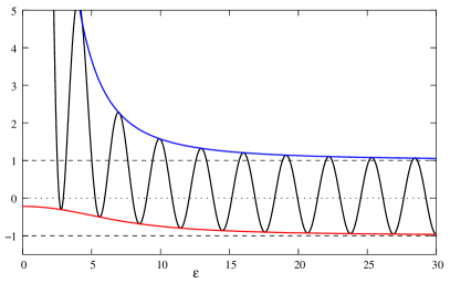
(a) $r_{1}=5$, $s_{1}=4$

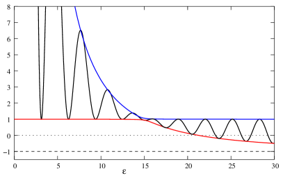
(b) $r_{1}=0.5$, $s_{1}=15$

Figure 1: Band condition for $N=2$ when $s\sim r$ and $s\gg r$. The coloured lines corresponds to $C_{\pm}$.

From the equation $\rmd\mathcal{B}/\rmd\varepsilon=0$ one can find the value of the oscillatory part of the band condition (i.e. the trigonometric functions) as a function of $\varepsilon$ and substituting into $\mathcal{B}$ with a properly choice of signs will result in an analytical form for the curves crossing the extremal points of the band condition which reads:

$$C_{\pm}=2\;f_{\pm}f_{\pm}^{*}-1$$ (3.2)

where $C_{+}(C_{-})$ lays on the maxima(minima) and the functions $f_{\pm}$ are defined as follows:

$$f_{\pm}= \frac{1}{\sqrt{F_{\pm}}}\left[\sqrt{2}r_{1}(r_{1}-\rmi s_{1})\pm\left(F_{\pm}-2r_{1}^{2}\varepsilon^{2}\right)^{\frac{1}{2}}\right]$$ (3.3)

$$F_{\pm}= r_{1}^{2}+(r_{1}^{2}+s_{1}^{2})^{2}+2(r_{1}+r_{1}^{2}-s_{1}^{2})\varepsilon^{2}+\varepsilon^{4}\pm$$ (3.4)

$$(r_{1}-r_{1}^{2}-s_{1}^{2}+\varepsilon^{2})\left[(r_{1}+r_{1}^{2}+s_{1}^{2})^{2}+2(r_{1}+r_{1}^{2}-s_{1}^{2})\varepsilon^{2}+\varepsilon^{4}\right]^{\frac{1}{2}}.$$

Hence, the behaviour of the band condition can be studied through the evolution of $C_{\pm}$. Taking the limit $s_{1}\rightarrow 0$ we obtain,

$$\lim_{s_{1}\rightarrow 0}C_{\pm}=\cases{1+\frac{2r_{1}^{2}}{\varepsilon^{2}}\frac{r_{1}(2+r_{1})+\varepsilon^{2}}{r_{1}(2+r_{1})+\varepsilon^{2}+\frac{r_{1}^{2}}{\varepsilon^{2}}}\\ -1.}$$ (3.5)

The real part of the couplings controls the amplitude of the oscillations (and therefore the distance between $C_{+}$ and $C_{-}$) but the minima will always lean on $\mathcal{B}=-1$ unless the imaginary part is non zero. Thus as we increase $s_{1}$ the minima will rise, as can be seen in figure 1(a), and they never touch $-1$ because $\lim_{\varepsilon\rightarrow\infty}C_{-}=-1$. On the other hand considering $r_{1}\rightarrow 0$, after some algebra one obtains

$$\lim_{r_{1}\rightarrow 0}C_{+} =\cases{-1+\frac{2s_{1}^{2}}{\varepsilon^{2}}\frac{s_{1}^{4}+\varepsilon^{4}+s_{1}^{2}(1-2\varepsilon^{2})}{s_{1}^{4}+\varepsilon^{4}+s_{1}^{2}(\frac{s_{1}^{2}}{\varepsilon^{2}}-2\varepsilon^{2})}&for $\varepsilon\leq s_{1}$\\ 1&for $\varepsilon>s_{1}$}$$ (3.6)

and for $C_{-}$ the limit is the same as for $C_{+}$ but interchanging with respect to the intervals in $\varepsilon$. Thus for an imaginary part of the coupling large enough compared to the real one the band condition goes above $+1$ for energies below the value $s_{1}$. Figure 1(b) shows this last configuration. In fact the situation $s_{1}\gg r_{1}$ can be easily understood from the form of the band condition that can easily be written in this limit as:

$$\mathcal{B}\simeq-1+\frac{2s_{1}^{2}}{\varepsilon^{2}}+2\cos^{2}(x)\left(1-\frac{s_{1}^{2}}{\varepsilon^{2}}\right)$$ (3.7)

which shows clearly the boundaries when $\varepsilon\leq s_{1}:\,1\leq\mathcal{B}\leq-1+2s_{1}^{2}/\varepsilon^{2}$ saturated at $\varepsilon=n\pi$ and $\varepsilon=(2n+1)\frac{\pi}{2}\quad n\in\mathbb{Z}$ respectively. For $\varepsilon>s_{1}$ the boundaries simply interchange among them. Due to the nature of the functions $h_{j}(\varepsilon)$ the band condition is always tied up to the value $+1$ at every multiple of $\pi$ for all $r_{1},s_{1}$, as figure 1(b) clearly shows. Several configurations of the spectrum as the ones in figure 1 can be built for different values of the complex coupling.

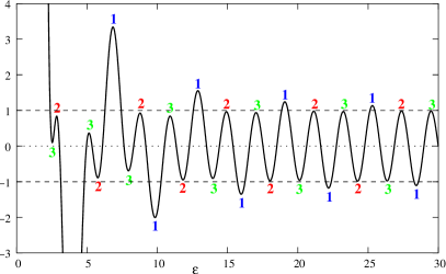
(a) $r_{1}=4$, $r_{2}=5$, $s_{1}=3$

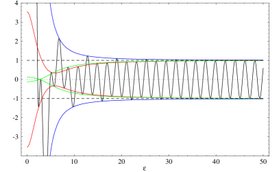
(b) $r_{1}=3$, $r_{2}=2$, $s_{1}=5$

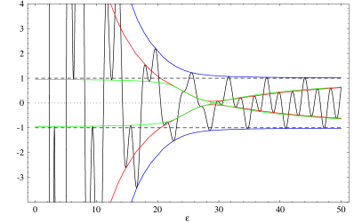
(c) $r_{1}=3$, $r_{2}=2$, $s_{1}=25$

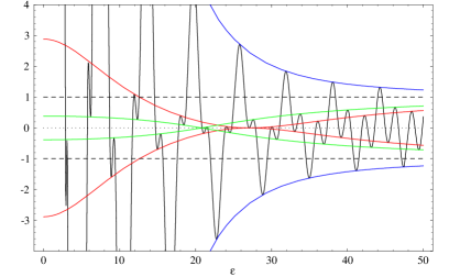
(d) $r_{1}=10$, $r_{2}=10$, $s_{1}=25$

Figure 2: Band condition for $N=3$ for different values of the couplings. Each type of extremal point is labelled with a different colour.

Let us now consider a $\mathcal{PT}$-symmetric chain whose primitive cell includes $3$ atoms charaterized by the parameters $(a/a_{1})=r_{1}+\rmi s_{1}$, $(a/a_{2})=r_{2}$ and $(a/a_{1})^{*}$. The band condition function reads $\mathcal{B}=4\;h_{1}h_{1}^{*}h_{2}-(h_{1}+h_{1}^{*}+h_{2})$. This can be arranged as:

$$\mathcal{B}=\mathcal{B}(s_{1}=0)+\frac{4s_{1}^{2}\sin^{2}(\varepsilon)\left[\varepsilon\cos(\varepsilon)+r_{2}\sin(\varepsilon)\right]}{\varepsilon^{3}}.$$ (3.8)

The extra term arising from the imaginary part of the coupling can be either positive or negative depending on the value of $r_{2}$ and the energy. The effect of $s_{1}$ is different compared to the previous case although there is only one imaginary parameter. The structure of the band condition seems to be composed by pieces each one including $3$ different types of extremal points, as figure 2(a) shows, and each type apparently following a given pattern. The curves crossing the extremal points of the band condition can also be analytically calculated in this $N=3$ case but the expressions are quite hard to simplify and therefore we do not provide the explicit form of the equations. Three curves are obtained, one for each type of extremal point. Initially when $s_{1}=0$ all the extremal points are outside or on the borders of the range $[-1,1]$. As we increase the imaginary part, the amplitudes of two of the three types of extremal points begin to decrease (green and red in figure 2(b)). At the same time as $s_{1}$ becomes larger the green and red curves get narrower with decreasing energy until $\varepsilon\sim s_{1}$. Below this value the curves broaden trying to expel the extremal points of the band condition outside the target range (figure 2(c)). From the form of $\mathcal{B}$ it is clear that the even(odd) multiples of $\pi$ will remain fixed to $1$($-1$). The efficiency of this expelling process depends upon the values of the real couplings as they control the amplitudes of the oscillations. One can stretch the maxima and minima (up and down respectively) increasing $r_{1}$, $r_{2}$, as shown in figure 2(d).

Several configurations can be obtained among the ones shown in figure 2 and one important feature must be emphasized: the band condition always changes “symetrically” with respect to the abscisa axis. That is: there is the same amount of positive and negative function whatever the values of the couplings are. In fact the curves laying on the extremal points show an exact reflection symmetry around the energy axis. This is in great contrast to the $N=2$ case where the band condition can be pushed up above $+1$ for certain couplings. Thus when $s_{1}\gg r_{1},r_{2}$ there will always remain a trace of the original permitted energy ranges in the form of “flat” bands.

(a) $r_{1}=3$, $r_{2}=2$, $s_{1}=0$, $s_{2}=0$

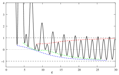
(b) $r_{1}=3$, $r_{2}=2$, $s_{1}=9$, $s_{2}=2$

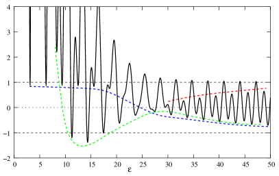
(c) $r_{1}=3$, $r_{2}=2$, $s_{1}=4$, $s_{2}=25$

(d) $r_{1}=3$, $r_{2}=2$, $s_{1}=20$, $s_{2}=21$

Figure 3: Band condition for $N=4$ with different values of the couplings. The coloured dashed lines are intended to clarify the behaviour of different groups of extremal points.

The first chain for which two different imaginary couplings can be manipulated is the one with $N=4$ atoms inside the primitive cell: $(a/a_{1})=r_{1}+\rmi s_{1}$, $(a/a_{2})=r_{2}+\rmi s_{2}$, $(a/a_{2})^{*}$ and $(a/a_{1})^{*}$. In this case we have not calculated analytically the curves crossing the extremal points. Nevertheless a pictorial approach for some of the curves has been included in the graphics for a better understanding of the tendencies of change. The initial situation ($s_{1}=s_{2}=0$) is a common one for a periodic chain (figure 3(a)) and two different group of extremal points can be distinguished. As we increase the imaginary part of the couplings one group of extremal points starts to decrease and the band condition lifts up globally (figure 3(b)). The effect of the two imaginary parts is quite similar. When both of them have comparable values the two groups of minima follow the same tendency moving upwards the band condition. However if one imaginary part grows much more than the other one, several minima strech down in a region of energy roughly included in $s_{small}<\varepsilon<s_{large}$ (figure 3(c)). Finally when $s_{1},s_{2}\gg r_{1},r_{2}$ one can force the band condition to go above $+1$ (keeping our well known knots at $\varepsilon=n\pi$) in a certain energy range which depends on the values of the imaginary parts of the couplings (figure 3(d)) approximately the same way as for the $N=2$ case. Unlike the $N=3$ example the band condition can be unbalanced to positive values with a properly choice of the parameters.

The band condition has been also studied in detail for $N=5$ and $N=6$. Its behaviour gets really complex as the number of atoms grows. In figure 4 and figure 5 some characteristic examples are shown. For $N=5$ the band condition shows five types of extremal points that evolve “symmetrically” around the abcisa axis as we change the imaginary couplings. For $N=6$ three types of maxima and minima appear and for large enough values of the imaginary couplings the band condition is greater than $+1$.

To summarize this mathematical analysis of the band condition let us now list some of the most salient features:

• the band condition is composed of pieces integrated by $N$($N/2$) extremal points for odd(even) $N$. Each extremal point belongs to a group that evolves differently according to the values of the imaginary parts of the couplings

• for odd $N$ the band condition is “symmetric” around the abcisa axis for all values of the couplings. Therefore, some permitted levels always remain as a part of the spectrum

• for even $N$ the band condition can be expelled out of the target range for certain values of the couplings and so removing the allowed bands

• for $\varepsilon=n\pi$ the band condition is fixed to $+1$ or $-1$ depending on the parity of $N$ and $n$ for all values of the couplings

• the real parts of the couplings are always proportional to the amplitude of the oscillations.

(a) $r_{1}=4$, $r_{2}=1$, $r_{3}=1$, $s_{1}=20$, $s_{2}=5$

(b) $r_{1}=4$, $r_{2}=2$, $r_{3}=3$, $s_{1}=10$, $s_{2}=20$

Figure 4: Band condition for a $\mathcal{PT}$-symmetric chain with $N=5$.

(a) $r_{1}=5$, $r_{2}=3$, $r_{3}=4$, $s_{1}=2$, $s_{2}=5$, $s_{3}=4$

(b) $r_{1}=1$, $r_{2}=2$, $r_{3}=0.5$, $s_{1}=10$, $s_{2}=11$, $s_{3}=12$

Figure 5: Band condition for a $\mathcal{PT}$-symmetric chain with $N=6$.

Even with all the included figures it is hard to make a complete explanation of the behaviour of the band condition that otherwise can only be fully understood watching some proper animations of the function. This is the procedure we have followed to support the results. We encourage the interested reader to reproduce those animations that can easily be done with Mathematica. Some example code lines are listed in the appendix.

4 The band structure and the electronic states

Let us now make some comments about the band structure. One important feature that stands out from the above examples is the presence of maxima(minima) inside the target range $(-1,1)$. This fact involves the presence of points in the recripocal space where the gradient of the energy diverges that makes the physical interpretation of the hamiltonian not so straightforward. Probably some additional restrictions have to be imposed on the $\mathcal{PT}$-symmetric hamiltonian. These special points also cause some changes on the form of the bands which are always understood as the ensembles of states and energies labelled with a certain index ($n$ for the $n$-th band). Every point of the Brillouin zone must represent a physical state on every band. Therefore for a certain value $Qa$ let us label the eigenenergies of the hamiltonian following an increasing order ($\varepsilon_{1}(Qa)<\varepsilon_{2}(Qa)<\ldots$). These procedure leads unavoidably to the definition of bands whose dipersion relations are not continuos over the reciprocal space as seen in figure 6(a). Of course the choice of the bands indices is not unique but none of them will be free of these discontinuities.

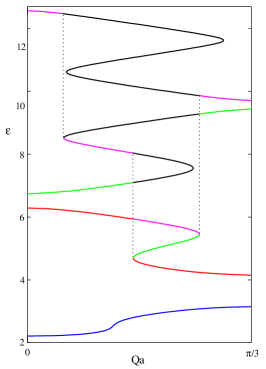
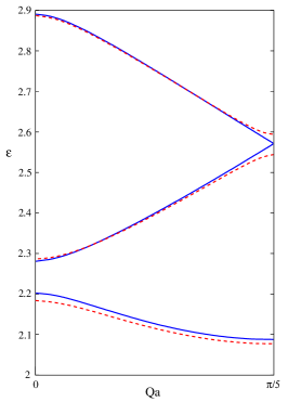
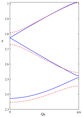
Figure 6: Band structure in the irreducible part of the first Brillouin zone for different chains: (a) $N=3$ with $r_{1}=1$, $r_{2}=2$, $s_{1}=3$. Different colours show the first four bands. (b) $N=5$ with $r_{1}=4$, $r_{2}=2$, $r_{3}=1$, $s_{1}=s_{2}=0$ (red) and $s_{1}=0.775$, $s_{2}=0.1$ (blue). (c) $N=6$ with $r_{1}=5$, $r_{2}=2$, $r_{3}=3$, $s_{1}=s_{2}=s_{3}=0$ (red) and $s_{1}=1.613$, $s_{2}=0.12$, $s_{3}=0.3$ (blue).

On the other hand those pathologies can be avoided if one restrics his working scenario to an small range of energies. In that case the imaginary parts of the couplings can be tuned to modify essentially the spectrum of the system removing or decreasing gaps to change virtually its response to transport phenomena (figures 6(b) and 6(c)).

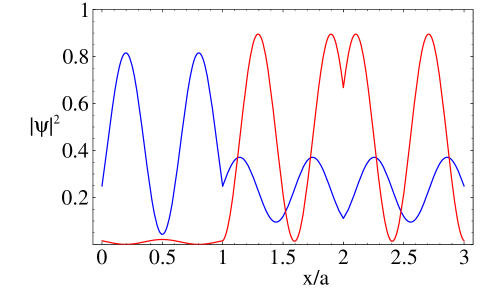
Figure 7: Electronic wave function normalized to 1 inside the primitive cell of a $\mathcal{PT}$-symmetric chain for $N=3$ with $r_{1}=5$, $r_{2}=3$. $s_{1}=0$(blue) and $s_{1}=19$(red) at $\varepsilon=5.2$.

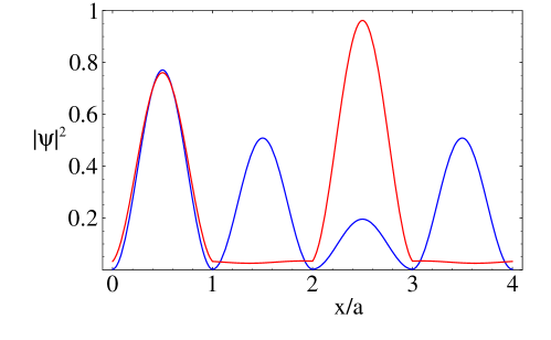
Figure 8: Electronic wave function normalized to 1 inside the primitive cell of a $\mathcal{PT}$-symmetric chain for $N=4$ with $r_{1}=3$, $r_{2}=4$, $s_{1}=5$, $s_{2}=8.1$ for different energies: $\varepsilon=2.95$(red) and $\varepsilon=3.13$(blue).

One can also wonder about the form of an electronic states belonging to such a characteristic spectrum. It is not hard to calculate analytically the wave function inside the primitive cell as a function of the position and the energy with the help of the computer for low $N$. To our surprise we have found that the imaginary parts of the couplings behave as control parameters of the localization of the electrons inside the primitive cell. Thus one could tune these parameters to decrease the probability of presence in several sectors almost to zero or distribute it more homogeneously over the primitive cell, as shown in figure 7. Also for non-vanishing imaginary parts of the couplings the depence of the state on the energy seems quite strong as a small variation of this energy can involve an important change in the shape of the state (figure 8).

5 Conclusions

In this paper the band structure of a one dimensional $N$-different coupling delta periodic potential is also assumed to be $\mathcal{PT}$-symmetric and hence the delta couplings can be made complex. In spite of the non-hermitian nature of such a Hamiltonian, the band spectrum condition remains real. The imaginary parts of the couplings play an essential role in the variety of shapes and forms that the band spectrum and the wavefunctions may acquire in this new framework. Although the band condition is analytical for arbitrary $N$, we have studied carefully just some cases with a low number of couplings. A throughout study of the $N=2$ case is given with analytic expressions for the limiting points of the bands. The cases $N=3$, $4$, $5$ and $6$ are solved graphically and conclusive results for the band spectrum are also offered. In all these cases, the control of the imaginary parts plays an essential role in the way that the band spectrum gets distorted and reshaped. As we have been able to discuss the evolution of this band spectrum, we are now planning to apply these results to more physical situations in which localization and de-localization may be tuned on and off by means of a judicious control of the imaginary parts. We have been able to show how wavefunction de-localization takes place actually for particular cases as the ones discussed in Section 4. However a manifold of interest questions remains to be answered such as: Could a random (non-periodical) calculation with this sort of potentials be carried out in the case of $\mathcal{PT}$-symmetry ?, Does the de-localization property holds for more general cases?. These and related research subjects are now being investigated and will be reported elsewhere.

Appendix

Here are some example lines for animating the band condition. First load the package “Animation” and define the band conditions for $N=2$ and $N=3$.

    << Graphics ‘Animation‘
    h[r_,s_]=Cos[x]+(r+I*s)*Sin[x]/x;
    B2[r1_,s1_]=2*h[r1,s1]*h[r1,-s1]-1;
    B3[r1_,r2_,s1_]=4*h[r1,s1]*h[r2,0]*h[r1,-s1]
                         -(h[r1,s1]+h[r2,0]+h[r1,-s1]);

To see the evolution of the band condition for $N=3$ versus the imaginary part $s_{1}$ for $r_{1}=2$ and $r_{2}=3$ one would write:

    Animate[Plot[Evaluate[{B3[2,3,t],1,-1}],{x,0,30},
                                         PlotRange->{-3,3}],{t,0,30}]

and finally one must group and compress the cells with all the generated plots and by double clicking on the image the animation will start.

References

References

- [1] Cerveró José M and Rodriguez A 2002 Eur. Phys. J., B 30 239-251
- [2] Cerveró José M and Rodriguez A 2003 Eur. Phys. J., B 32 537-543
- [3] Bender Carl M and Boettcher S 1998 Phys. Rev. Lett., 80 5243-5246
- [4] Cerveró José M 2003 Phys. Lett., A 317 26-31
- [5] Avinash Khare et al. 1998 J. Phys. A: Math. Gen., 21 L501-L508
- [6] Cerveró José M 1991 Phys. Lett., A 153 1-4
- [7] Lévay G and Znojil M 2002 J. Phys. A: Math. Gen., 35 8793-8804
- [8] Znojil M 2003 J. Phys. A: Math. Gen., 36 7639-7648
- [9] Mostafazadeh A 2003 Preprint quant-ph/0310164
- [10] Ram Narayan Deb et al. 2003 Phys. Lett., A 307 215-221
- [11] Bender Carl M et al. 1999 Phys. Lett., A 252 272-276
- [12] Ahmed Zafar 2001 Phys. Lett.A, 286 231-235