Dynamical tunneling of bound systems through a potential barrier: complex way to the top.

Abstract

A semiclassical method of complex trajectories for the calculation of the tunneling exponent in systems with many degrees of freedom is further developed. It is supplemented with an easily implementable technique, which enables one to single out the physically relevant trajectory from the whole set of complex classical trajectories. The method is applied to semiclassical transitions of a bound system through a potential barrier. We find that the properties of physically relevant complex trajectories are qualitatively different in the cases of potential tunneling at low energy and dynamical tunneling at energies exceeding the barrier height. Namely, in the case of high energies, the physically relevant complex trajectories describe tunneling via creation of a state close to the top of the barrier. The method is checked against exact solutions of the Schrödinger equation in a quantum mechanical system of two degrees of freedom.

I Introduction

Semiclassical methods provide a useful tool for the study of nonperturbative processes. Tunneling phenomena represent one of the most notable cases where semiclassical techniques are used to obtain otherwise unattainable information on the dynamics of the transition. A standard example of semiclassical technique is WKB approximation to tunneling in quantum mechanics of one degree of freedom. In this case solutions $S(q)$ to the Hamilton–Jacobi equation are pure imaginary in the classically forbidden region. Therefore, the function $S(q)$ can be obtained as the action functional on a real trajectory $q(\tau)$, which is the solution to the equations of motion in Euclidean time domain, $t=-i\tau$, with real Euclidean action $S_{E}=-iS$.

This simple picture of tunneling is no longer valid for systems with many degrees of freedom, where solutions $S(\mathbf{q})$ to the Hamilton–Jacobi equation are known to be generically complex in the classically forbidden region (see Refs. Huang:1989 ; Takada:1993 for recent discussion). This leads to the concept of “mixed” tunneling, as opposed to “pure” tunneling where $S(\mathbf{q})$ is pure imaginary. “Mixed” tunneling cannot be described by any real tunneling trajectory. However, it could be related to a complex trajectory. If so, the function $S(\mathbf{q})$ (and therefore the exponential part of the wave function) is calculated as the action functional on this complex trajectory.

A particularly difficult situation arises when one considers transitions of a non–separable system with a strong interaction between its degrees of freedom, such that the quantum numbers of the system change considerably during the transition. Methods based on adiabatic expansion are not applicable in this situation, while the method of complex trajectories proves to be extremely useful.

The method of complex trajectories in the form suitable for the calculation of $S$–matrix elements was formulated and checked by direct numerical calculations in Refs. Miller:1970 ; Miller:1972 ; George:1972 (see Ref. Miller for review). Further studies Wilkinson:1986 ; Wilkinson:1987 ; Takada:1995 ; Takada:1996 ; Bonini:1999cn ; Bonini:1999kj showed that this method can be generalized to the calculation of the tunneling wave functions and tunneling probabilities, energy splittings in double well potentials and decay rates from metastable states. Similar methods were successful in the study of tunneling in high-energy collisions in field theory Rubakov:1992ec ; Kuznetsov:1997az ; Bezrukov:2001dg ; Bezrukov:2003er , where one considers systems with definite particle number (${\cal N}=2$) in the initial state; in the study of chemical reactions and atom ionization processes, where the initial bound systems are in definite quantum states Miller ; Perelomov1 ; Perelomov2 ; etc. The main advantage of the method of complex trajectories is that it can be easily generalized and numerically implemented in the cases of large and even infinite (field theory) number of degrees of freedom, in contrast to other methods such as Huygens-type construction of Refs. Huang:1989 ; Takada:1993 and initial value representation (IVR) of Refs. Miller:1970 ; Miller:1988 ; Thompson:1999 ; Kay:1997 ; Maitra:1997 ; Miller:2001 .

In this paper we develop the method of complex trajectories further. Namely, we concentrate on the following problem. It is known Miller:1970 that the physically relevant complex trajectory satisfies the classical equations of motion with certain boundary conditions. However, this boundary value problem generically has also an infinite, though discrete, set of unphysical solutions. In one dimensional quantum mechanics all solutions can easily be classified. In systems with many degrees of freedom such a classification is extremely difficult, if at all possible. In the case of small number of degrees of freedom (realistically, $N=2$), one can scan over all solutions and find the solution giving the largest tunneling probability Miller:1970 ; Takada:1995 ; Takada:1996 , but in systems with large or infinite number of degrees of freedom the problem of choosing the physically relevant solution becomes a formidable task.

The problem of choosing the appropriate solution becomes even more pronounced when the qualitative properties of the relevant complex trajectory are different in different energy regions. This may happen when the physically relevant classical solution “meets” an unphysical one at some value of energy $E=E_{1}$, or in other words, when solutions to the boundary value problem, viewed as functions of energy, bifurcate at $E=E_{1}$.

In this paper we give an example of this sort, which appears to be fairly generic (see also Bonini:1999cn ; Bonini:1999kj ; Kuznetsov:1996cm ; Bezrukov:2001dg ; Bezrukov:2003er ). We then develop a method which chooses the phyically relevant solution automatically, implement it numerically and check this method against the numerical solution to the full Schrödinger equation.

We study inelastic transitions of a bound system through a potential barrier. For concreteness we consider a model with one internal degree of freedom besides the center-of-mass coordinate. We consider a situation in which the spacing between the levels of the bound system is small compared to the height of the barrier, and assume strong enough coupling between the degrees of freedom, to make sure that the quantum numbers of the bound system change considerably during the transition process. This is precisely the situation in which the method of complex trajectories shows its full strength.

Transitions of bound systems involve a particular energy scale — the height of the barrier $V_{0}$. At energies below $V_{0}$ classical over–barrier transitions are forbidden energetically; the corresponding regime is called “potential tunneling”. For $E>V_{0}$ it is energetically allowed for the system to evolve classically to the other side of the barrier. However, over-barrier transitions may be forbidden dynamically even at $E>V_{0}$. Indeed, inelastic interactions of a bound system with a potential barrier generally lead to the excitation of the internal degrees of freedom with the simultaneous decrease of the center-of-mass energy, and this may prevent the system from the over–barrier transition. Tunneling regime at energies exceeding the barrier height is called “dynamical tunneling”.

Examples of dynamical tunneling are well–known in scattering theory Miller:1972 . This type of tunneling between bound states was discovered in Ref. Heller:1981 , the generality of dynamical tunneling in large molecules was stressed in Refs. Davis:1981 ; Heller:1994 . It is dynamical tunneling that is of primary interest in our study.

A novel phenomenon we observe is that dynamical tunneling at $E\gtrsim V_{0}$ (more precisely, at $E>E_{1}$, where $E_{1}$ is somewhat larger than $V_{0}$) occurs in the following way: the system jumps on top of the barrier, and restarts its classical evolution from the region near the top. From the physical viewpoint, this is not quite what is normally meant by “tunneling through a barrier”. Yet the transitions remain exponentially suppressed, but the reason is different: to jump above the barrier, the system has to undergo considerable rearrangement, unless the incoming state is chosen in a special way (see footnote, above). This rearrangement costs exponentially small probability factor. We note that similar exponential factor was argued to appear in various field theory processes with multi-particle final states Banks:1990zb ; Zakharov:1991rp ; Veneziano:1992rp ; Rubakov:1995hq .

We find that the new physical behaviour of the system is related to a bifurcation of the family of the complex-time classical solutions, viewed as functions of energy. This is precisely the bifurcation which we alluded to above. Our method of dealing with this bifurcation is to regularize the boundary value problem in such a way that the bifurcations disappear altogether (at real energies), and the only solutions recovered after removing the regularization are physical ones.

The paper is organized as follows. The system we discuss in this paper is introduced in Sec. II.1. In Sec. II.2 we formulate the boundary value problem for the calculation of the tunneling exponent. Then we examine the classical over-barrier solutions and find all initial states that lead to classically allowed transitions in Sec. II.3. In Sec. II.4 we present a straightforward application of the semiclassical technique, outlined in Sec. II.2, and find that it ceases to produce relevant complex trajectories n a certain region of initial data, namely, at $E>E_{1}$. In Sec. III we introduce our regularization technique and show that it indeed enables one to find all the relevant complex trajectories, including ones with $E>E_{1}$ (Sec. III.1). We check our method against the numerical solution of the full Schrödinger equation in Sec. III.2. In Sec. III.3 and Appendix C we show how our regularization technique is used to join smoothly the “classically allowed” and “classically forbidden” families of solutions in the cases of two- and one- dimensional quantum mechanics, respectively.

II Semiclassical transitions through a potential barrier

II.1 The model

The situation we discuss in this paper is a transition through a potential barrier of a bound system of Refs. Bonini:1999cn ; Bonini:1999kj , namely a system made of two particles of identical mass $m$, moving in one dimension and bound by a harmonic oscillator potential of frequency $\omega$ (Fig. 1).

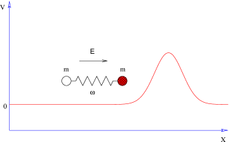
Figure 1: Oscillator hitting a potential barrier, with which only the “dark” particle interacts.

One of the particles interacts with a repulsive potential barrier. The potential barrier is assumed to be high and wide, while spacing between the oscillator levels is much smaller than the barrier height $V_{0}$. The Hamiltonian of the model is

$$H=\frac{p_{1}^{2}}{2m}+\frac{p_{2}^{2}}{2m}+\frac{m\omega^{2}}{4}(x_{1}-x_{2})^{2}+V_{0}\mathrm{e}^{-x_{1}^{2}/2\sigma^{2}}\;,$$ (1)

where the conditions on the oscillator frequency and potential barrier are

$$\hbar\omega\ll V_{0},$$ (2)

$$\sigma\gg\hbar/\sqrt{mV_{0}}\;.$$

Since the variables do not separate, this is certainly a non-trivial system.

We choose units with $\hbar=1,$ $m=1$. It is also convenient to treat the frequency $\omega$ as a dimensionless parameter, so that all physical quantities are dimensionless. In our subsequent numerical study we use the value $\omega=0.5$, still keeping, however, notation “$\omega$” in formulas. The system is semiclassical, i.e.  conditions (2) are satisfied, if one chooses $\sigma=1/\sqrt{2\lambda}$, $V_{0}=1/\lambda$, where $\lambda$ is a small parameter. At the classical level, this parameter is irrelevant: after rescaling the variables $x_{1}\to x_{1}/\sqrt{\lambda},\;\;x_{2}\to x_{2}/\sqrt{\lambda},$ the small parameter enters only through the overall multiplicative factor $1/\lambda$ in the Hamiltonian. Therefore, the semiclassical technique can be developed as an asymptotic expansion in $\lambda$.

The properties of the system are made clearer by replacing the variables $x_{1},\;x_{2}$ with the center-of-mass coordinate $X\equiv(x_{1}+x_{2})/\sqrt{2}$ and the relative oscillator coordinate $y\equiv(x_{1}-x_{2})/\sqrt{2}$. In terms of the latter variables, the Hamiltonian takes the form

$$H=\frac{p_{X}^{2}}{2}+\frac{p_{y}^{2}}{2}+\frac{\omega^{2}}{2}y^{2}+\frac{1}{\lambda}\mathrm{e}^{-\lambda(X+y)^{2}/2}.$$ (3)

The interaction potential

$$U_{\mathrm{int}}\equiv\frac{1}{\lambda}\mathrm{e}^{-\lambda(X+y)^{2}/2}$$

vanishes in the asymptotic regions $X\to\pm\infty$ and describes a potential barrier between these regions. At $X\to\pm\infty$ the Hamiltonian (3) corresponds to an oscillator of frequency $\omega$ moving along the center-of-mass coordinate $X$. The oscillator asymptotic state is characterized by its excitation number $N$ and total energy $E=p_{X}^{2}/2+\omega(N+1/2)$. We are interested in the transmissions through the potential barrier of the oscillator with given initial values of $E$ and $N$.

II.2 $T/\theta$ boundary value problem

The probability of tunneling from a state with fixed initial energy $E$ and oscillator excitation number $N$ from the asymptotic region $X\to-\infty$ to any state in the other asymptotic region $X\to+\infty$ takes the following form:

$$\mathcal{T}(E,N)=\lim_{t_{f}-t_{i}\to\infty}\sum_{f}\left|\langle f|\mathrm{e}^{-i\hat{H}(t_{f}-t_{i})}|E,N\rangle\right|^{2}\;,$$ (4)

where it is implicit that the initial and final states have support only well outside the range of the potential, with $X<0$ and $X>0$, respectively. Semiclassical methods are applicable when the initial energy and excitation number are parametrically large,

$$E=\tilde{E}/\lambda\;,\quad N=\tilde{N}/\lambda\;,$$

where $\tilde{E}$ and $\tilde{N}$ are held constant as $\lambda\to 0$. The transition probability has the exponential form

$${\cal T}=D\mathrm{e}^{-\frac{1}{\lambda}F(\tilde{E},\;\tilde{N})}\;,$$ (5)

where $D$ is a pre-exponential factor, which is not considered in this paper. Our purpose is to calculate the leading semiclassical exponent $F(\tilde{E},\;\tilde{N})$. The exponent for tunneling from the oscillator ground state is obtained Rubakov:1992fb ; Rubakov:1992ec ; Bonini:1999cn ; Bonini:1999kj by taking the limit ${\tilde{N}\to 0}$ in $F(\tilde{E},\tilde{N})$.

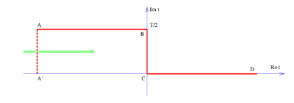
Figure 2: Contour in the complex time plane.

In what follows we rescale the variables, $X\to X/\sqrt{\lambda}$, $y\to y/\sqrt{\lambda}$, and omit tilde over the rescaled quantities $\tilde{E},\;\tilde{N}$.

The exponent $F(E,N)$ is related to a complex trajectory, which satisfies a certain complexified classical boundary value problem. We present the derivation of this problem in Appendix A. The outcome is as follows. There are two Lagrange multipliers, $T$ and $\theta$, which are related to the parameters $E$ and $N$ characterizing the incoming state. The boundary value problem is conveniently formulated on the contour ABCD in the complex time plane (see Fig. 2), with the imaginary part of the initial time equal to $T/2$. The coordinates $X(t),\;y(t)$ must satisfy the complexified equations of motion in the internal points of the contour, and be real in the asymptotic future (region D):

$$\frac{\delta S}{\delta X(t)}=\frac{\delta S}{\delta y(t)}=0\;,$$ (6a)

$$\begin{array}[]{l}\displaystyle\mathop{\mathrm{Im}}y(t)\to 0,\\[4.30554pt] \displaystyle\mathop{\mathrm{Im}}X(t)\to 0,\end{array}\qquad\text{as }t\to+\infty\;.$$ (6d)

In the asymptotic past (region A of the contour, where $$t=t^{\prime}+iT/2 t^{\prime} U_{\mathrm{int}}$$, is real negative) one can neglect the interaction potential , and the oscillator decouples:

$$y=\frac{1}{\sqrt{2\omega}}(u\mathrm{e}^{-i\omega t^{\prime}}+v\mathrm{e}^{i\omega t^{\prime}}).$$

The boundary conditions in the asymptotic past, $$t^{\prime}\to-\infty X$$, are that the center-of-mass coordinate must be real, while the complex amplitudes of the decoupled oscillator must be linearly related,

$$\begin{array}[]{l}\mathop{\mathrm{Im}}X\to 0,\\[4.30554pt] v\to\mathrm{e}^{\theta}u^{*},\end{array}\qquad\text{as }t^{\prime}\to-\infty\;.$$ (6e)

The boundary conditions (6d) and (6e) make, in fact, eight real conditions (since, e.g., $\mathop{\mathrm{Im}}X(t^{\prime})\to 0$ implies that both $\mathop{\mathrm{Im}}X$ and $\mathop{\mathrm{Im}}\dot{X}$ tend to zero), and completely determine a solution, up to time translation invariance (see discussion in Appendix A).

It is shown in Appendix A that a solution to this boundary value problem is an extremum of the functional

$$F[X,y;X^{*},y^{*};T,\theta]=-iS[X,y]+iS[X^{*},y^{*}]\\ -ET-N\theta+\text{Boundary terms}\;.$$ (7)

The value of this functional at the extremum gives the exponent for the transition probability (up to large overall factor $1/\lambda$, see eq. (5)),

$$F(E,\;N)=2\mathop{\mathrm{Im}}S_{0}(T,\;\theta)-ET-N\theta\;,$$ (8)

where $S_{0}$ is the action of the solution, integrated by parts,

$$S_{0}=\int\!dt\left(\!-\frac{1}{2}X\frac{d^{2}X}{dt^{2}}-\frac{1}{2}y\frac{d^{2}y}{dt^{2}}\right.\\ \left.-\frac{1}{2}\omega^{2}y^{2}-U_{\mathrm{int}}(X,y)\right).$$ (9)

Here the integration runs along the contour ABCD. The values of the Lagrange multipliers $T$ and $\theta$ are related to energy and excitation number as follows,

$$E(T,\theta) = \frac{\partial}{\partial T}2\mathop{\mathrm{Im}}S_{0}(T,\theta)\;,$$ (10)

$$N(T,\theta) = \frac{\partial}{\partial\theta}2\mathop{\mathrm{Im}}S_{0}(T,\theta)\;.$$ (11)

Making use of Eq. (8), it is straightforward to check also the inverse Legendre transformation formulas,

$$T(E,\;N) = -\frac{\partial}{\partial E}F(E,\;N)\;,$$ (12)

$$\theta(E,\;N) = -\frac{\partial}{\partial N}F(E,\;N)\;.$$ (13)

One can also check that the right hand side of Eq. (10) coincides with the energy of the classical solution, while the right hand side of Eq. (11) is equal to the classical counterpart of the occupation number,

$$E=\frac{\dot{X}^{2}}{2}+\omega N\;;\qquad N=uv\;.$$ (14)

So, one may either search for the values of $T$ and $\theta$ that correspond to given $E$ and $N$, or, following a computationally simpler procedure, solve the boundary value problem (6) for given $T$ and $\theta$ and then find the corresponding values of $E$ and $N$ from Eq. (14). Note that the initial conditions (6e) complemented by Eqs. (14) are equivalent to the initial conditions of Refs. Miller:1970 ; Miller:1972 ; George:1972 , the latter being expressed in terms of action–angle variables. The boundary conditions in the asymptotic future (6d) are different from those of Refs.Miller:1970 ; Miller:1972 ; George:1972 , since we consider inclusive, rather than fixed, final state.

Let us discuss some subtle points of the boundary value problem (6). First, one notices that the condition of asymptotic reality (6d) does not always coincide with the condition of reality at finite time. Of course, if the solution approaches the asymptotic region $X\to+\infty$ on the part CD of the contour, the asymptotic reality condition (6d) implies that the solution is real at any finite positive $t$. Indeed, the oscillator decouples as $X\to+\infty$, so the condition (6d) means that its phase and amplitude, as well as $X(t)$, are real as $t\to+\infty$. Due to equations of motion, $X(t)$ and $y(t)$ are real on the entire CD–part of the contour. This situation corresponds to the transition directly to the asymptotic region $X\to+\infty$. However, the situation can be drastically different if the solution on the final part of the time contour remains in the interaction region. For example, let us imagine that the solution approaches the saddle point of the potential $X=0$, $y=0$ as $t\to+\infty$. Since one of the perturbations about this point is unstable, there may exist solutions which approach this point exponentially along the unstable direction, i.e. $X(t),\;y(t)\propto\mathrm{e}^{-\mathrm{const}\cdot t}$ with possibly complex pre-factors. In this case the solution may be complex at any finite time, and become real only asymptotically, as $t\to+\infty$. Such solution corresponds to tunneling to the saddle point of the barrier, after which the system rolls down classically towards $X\to+\infty$ (with probability of order $1$, inessential for the tunneling exponent $F$). We will see in Sec. III.1 that the situation of this sort indeed takes place for some values of energy and excitation number.

Second, since at large negative time (in the asymptotic region $X\to-\infty$) the interaction potential disappears, it is straightforward to continue the asymptotics of the solution to the real time axis. For solutions satisfying (6e) this gives at large negative time

$$y(t)=\frac{1}{\sqrt{2\omega}}\left(u\mathrm{e}^{-\omega T/2}\mathrm{e}^{-i\omega t}+u^{*}\mathrm{e}^{\theta+\omega T/2}\mathrm{e}^{i\omega t}\right)\;,$$

$$\mathop{\mathrm{Im}}X(t)=-\frac{T}{2}p_{X}\;.$$

We see that the dynamical coordinates on the negative side of the real time axis are generally complex. For solutions approaching the asymptotic region $X\to+\infty$ as $t\to+\infty$ (so that $X$ and $y$ are exactly real at finite $t>0$), this means, that there should exist a branch point in the complex time plane: the contour A’ABC in Fig. 2 winds around this point and cannot be deformed to the real time axis. This argument does not work for solutions ending in the interaction region as $t\to+\infty$, so branch points between the AB–part of the contour and the real time axis may be absent. We will see in Sec. III.1 that this is indeed the case in our model in a certain range of $E$ and $N$.

II.3 Over-barrier transitions: the region of classically allowed transitions and its boundary $E_{0}(N)$

Before studying the exponentially suppressed transitions, let us consider the classically allowed ones. To this end, let us study the classical evolution (real time, real-valued coordinates), in which the system is initially located at large negative $X$ and moves with positive center-of-mass velocity towards the asymptotic region $X\to+\infty$. The classical dynamics of the system is specified by four initial parameters. One of them (e.g., the initial center-of-mass coordinate) fixes the invariance under time translation, while the other three are the total energy $E$, the initial excitation number of the $y$–oscillator, defined in classical theory as $N\equiv E_{\mathrm{osc}}/\omega$, and the initial oscillator phase $\varphi_{i}$.

Any initial quantum state of our system can be fully determined by energy $E$ and initial oscillator excitation number $N$; we can represent each state by a point in the $E$–$N$ plane. There is, however, one additional classically relevant initial parameter, the oscillator phase $\varphi_{i}$. An initial state $(E,N)$ leads to unsuppressed transmission if the corresponding classical over–barrier transitions are possible for some value(s) of $\varphi_{i}$. These states form some region in the $E$–$N$ plane, which is to be found in this section.

For given $N$, at large enough $E$ the system can certainly evolve to the other side of the barrier. On the other hand, if $E$ is smaller than the barrier height, the system definitely undergoes reflection. Thus, there exists some boundary energy $E_{0}(N)$, such that classical transitions are possible for $E>E_{0}(N)$, while for $E<E_{0}(N)$ they do not occur for any initial phase $\varphi_{i}$. The line $E_{0}(N)$ represents the boundary of the region of classically allowed transitions. We have calculated $E_{0}(N)$ numerically: the result is shown in Fig. 3.

An important point of the boundary $E_{0}(N)$ corresponds to the static unstable classical solution $X(t)=y(t)=0$. In field theory context, such a solution is called “sphaleron” Klinkhamer:1984di ), and for the sake of terminology we will use this name in what follows. This solution is the saddle point of the potential $U(X,y)\equiv{\omega^{2}y^{2}}/{2}+U_{\mathrm{int}}(X,y)$ and has exactly one unstable direction, the negative mode (see Fig. 4). The sphaleron energy $E_{\mathrm{S}}=U(0,0)=1$ determines the minimum value of the function $E_{0}(N)$. Indeed, while classical over–barrier transitions with ${E<E_{\mathrm{S}}}$ are impossible, the over–barrier solution with slightly higher energy can be obtained as follows: at the point $X=y=0$, one adds momentum along the negative mode, thus “pushing” the system towards $X\to+\infty$. Continuing this solution backwards in time one finds that the system tends to $X\to-\infty$ for large negative time and has a certain oscillator excitation number. Solutions with energy closer to the sphaleron energy correspond to smaller “push” and thus spend longer time near the sphaleron. In the limiting case when the energy is equal to $E_{\mathrm{S}}$, the solution spends an infinite time in the vicinity of the sphaleron. This limiting case has a definite initial excitation number $N_{\mathrm{S}}$, so that $E_{0}(N_{\mathrm{S}})=E_{\mathrm{S}}$ (see Fig. 3). The value of $N_{\mathrm{S}}$ is unique because there is exactly one negative direction of the potential in the vicinity of the sphaleron.

In complete analogy to the features of the over–barrier classical solutions near the sphaleron point ($E_{\mathrm{S}}$, $N_{\mathrm{S}}$), one expects that as the values of $E,\;N$ approach any other boundary point $(E_{0}(N),\;N)$, the corresponding over–barrier solutions will spend more and more time in the interaction region, where $U_{\mathrm{int}}\neq 0$. This follows from a continuity argument. Namely, let us first fix the initial and final times, $t_{i}$ and $t_{f}$. If in this time interval a solution with energy $E_{1}$ evolves to the other side of the barrier and a solution with energy $E_{2}$ and the same oscillator excitation number is reflected back, there exists an intermediate energy at which the solution ends up at $t=t_{f}$ in the interaction region. Taking the limit $t_{f}\to+\infty$ and $(E_{1}-E_{2})\to 0$, we obtain a point at the boundary $E_{0}(N)$ and a solution tending asymptotically to some unstable time dependent solution that spends infinite time in the interaction region. We call the latter solution excited sphaleron; it describes some (in general nonlinear) oscillations above the sphaleron along the stable direction in coordinate space. Therefore, every point of the boundary ${(E_{0}(N),\;N)}$ corresponds to some excited sphaleron. Solutions tending asymptotically to the excited sphalerons, form a surface in a phase space (separatrix), which separates regions of qualitatively different classical motion of the system.

We display in Fig. 4 a solution, found numerically in our model, that tends to an excited sphaleron. We see that the trajectory of excited sphaleron is, roughly speaking, orthogonal to the unstable direction at the saddle point $({X=0,}\;{y=0})$.

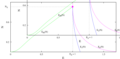
Figure 3: The boundary $E_{0}(N)$ of the region of classically allowed transitions, the bifurcation line $E_{1}(N)$ and the line of the periodic instantons $E_{PI}(N)$.

II.4 Suppressed transitions: bifurcation line $E_{1}(N)$

Let us now turn to classically forbidden transitions, and consider the boundary value problem (6). It is relatively straightforward to obtain numerically solutions for $\theta=0$. The boundary conditions (6d), (6e) in this case take the form of reality conditions in the asymptotic future and past. It can be shown Khlebnikov:1991th that the physically relevant solutions with $\theta=0$ are real on the entire contour ABCD of Fig. 2 and describe nonlinear oscillations in the upside-down potential on the Euclidean part BC of the contour. The period of the oscillations is equal to $T$, so that the points B and C are two different turning points, where $\dot{X}=\dot{y}=0$. These real Euclidean solutions are called periodic instantons. A practical technique for obtaining these solutions numerically on the Euclidean part BC consists in minimizing the Euclidean action (for example, with the method of conjugate gradients, see Ref. Bonini:1999cn ; Bonini:1999kj for details). The solutions on the entire contour are then obtained by solving numerically the Cauchy problem, forward in time along the line CD and backward in time along the line BA. Having the solution in asymptotic past (region A), one then calculates its energy and excitation number (14). The solutions to this Cauchy problem are obviously real, so the boundary conditions (6d), (6e) are indeed satisfied with $\theta=0$. It is worth noting that solutions with $\theta=0$ are similar to the ones in quantum mechanics of one degree of freedom. The line of periodic instantons in $E$–$N$ plane in our model is shown in Fig. 3.

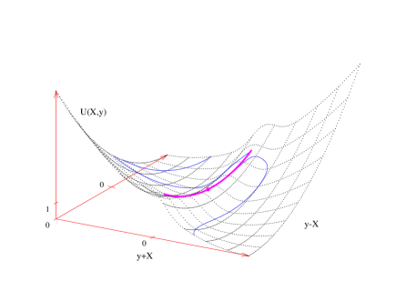
Figure 4: The potential (dotted lines) in the vicinity of the sphaleron ${(X=0,\;y=0)}$ (marked by the point), excited sphaleron (thick line) corresponding to the point $(E,N)=(1.985,3.72)$. at the boundary of the region of classically allowed transitions, and the trajectory of the solution which is close to this excited sphaleron (thin line). In this figure the asymptotic regions $X\to\pm\infty$ are along the diagonal.

Once the solutions with $\theta=0$ are found, it is natural to try to cover the entire region of classically forbidden transitions of $E-N$ plane with a deformation procedure, by moving in small steps in $\theta$ and $T$. The solution to the boundary value problem with $(T+\Delta T,\;\theta+\Delta\theta)$ may be obtained numerically, by applying an iteration technique, with the known solution at $(T,\;\theta)$ serving as the initial approximation. Provided the solutions end up in correct asymptotic region at each step, i.e. $X\to+\infty$ on part D of the contour, the solutions obtained by this procedure of small deformations are physically relevant. However, the method of small deformations fails to produce relevant solution if there are bifurcation points in the $E$–$N$ plane, where the physical branch of solutions merges to an unphysical branch. As there are unphysical solutions close to physical ones in the vicinity of bifurcation points, one cannot use the procedure of small deformations near these points.

We have found numerically that in our model the method of small deformations produces correct solutions to the $T/\theta$ boundary value problem in a large region of the $E-N$ plane, where $E<E_{1}(N)$. However, at sufficiently high energy $E>E_{1}(N)$, where $E_{1}(N)\gtrsim E_{\mathrm{S}}$, the deformation procedure generates solutions that bounce back from the barrier (see Fig. 5), i.e. have wrong “topology”.

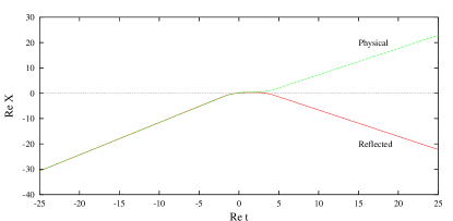
Figure 5: The dependence of the tunneling coordinate $X$ on time for two solutions with nearly the same energy and initial excitation number. The physical solution tunnels to the asymptotic region $X\to+\infty$, while the unphysical one gets reflected back to $X\to-\infty$. The physical solution has $E=1.028,\;N=0.44$, while the unphysical one has $E=1.034,\;N=0.44$. These two solutions are close to the point at the bifurcation line $E_{1}(N=0.44)=$ 1.031.

This happens deep inside the region of classically forbidden transitions, where the suppression is large, and one naively expects the semiclassical technique to work well. Clearly, solutions with wrong topology do not describe the tunneling transitions of interest. Therefore, if the semiclassical method is applicable at all in the region $E_{1}(N)<E<E_{0}(N)$, there exists another, physical branch of solutions. In that case the line $E_{1}(N)$ is the bifurcation line, where the physical solutions “meet” the ones with wrong “topology”. Walking in small steps in $\theta$ and $T$ is useless in the vicinity of this bifurcation line, and one needs to introduce some trick to find the relevant solutions beyond that line. The bifurcation line $E_{1}(N)$ for our quantum mechanical problem of two degrees of freedom is shown in Fig. 3.

The loss of topology beyond a certain bifurcation line in $E-N$ plane is by no means a property of our model only. This phenomenon has been observed in field theory models, in the context of both induced false vacuum decay Kuznetsov:1997az and baryon-number violating transitions in gauge theory Bezrukov:2001dg (in field-theoretic models, the parameter $N$ is the number of incoming particles). In all cases, the loss of topology prevented one to compute the semiclassical exponent for the transition probability in an interesting region of relatively high energies.

Coming back to quantum mechanics of two degrees of freedom, we point out that the properties of tunneling solutions with different energies approaching the bifurcation line $E_{1}(N)$ from the left of the $E$–$N$ plane, are in some sense similar to the properties of tunneling solutions in one–dimensional quantum mechanics whose energy is close to the barrier height, see Appendix C. Again by continuity, these solutions of our two-dimensional model spend a long time in the interaction region; this time tends to infinity on the line $E_{1}(N)$. Hence, at any point of this line, there is a solution which starts in the asymptotic region left of the barrier, and ends up on an excited sphaleron. Such a behavior is indeed possible because of the existence of an unstable direction near the (excited) sphaleron, even for complex initial data. We suggest in the next Section a trick to deal with this situation—this is our regularization technique.

III Regularization technique

In this Section we develop our regularization technique, and find the physically relevant solutions between the lines $E_{1}(N)$ and $E_{0}(N)$. We will see that all solutions from the new branch (and not only on the lines $E_{0}(N)$ and $E_{1}(N)$) correspond to tunneling onto the excited sphaleron (“tunneling on top of the barrier”). These solutions would be very difficult, if at all possible, to obtain directly, by solving numerically the non-regularized classical boundary value problem (6): they are complex at finite times, and become real only asymptotically as $t\to+\infty$, whereas numerical methods require working with finite time intervals.

As an additional advantage, our regularization technique enables one to obtain a family of the over–barrier solutions, that covers all the region of the initial data, corresponding to classicaly allowed transitions, including its boundary. This is of interest in models with large number of degrees of freedom and in field theory, where finding the boundary $E_{0}(N)$ by direct methods is difficult (see e.g., Ref. Rebbi:1995zw for discussion of this point).

III.1 Regularized problem: classically forbidden transitions

The main idea of our method is to regularize the equations of motion by adding a term proportional to a small parameter $\epsilon$ so that configurations staying for an infinite time near the sphaleron no longer exist among the solutions of the $T/\theta$ boundary value problem. After performing the regularization we explore all region of classically forbidden transitions without crossing the bifurcation line. Taking then the limit ${\epsilon\to 0}$ we reconstruct the correct values of $F$, $E$ and $N$.

When formulating the regularization technique it is more convenient to work with the functional $F[X,y;X^{*},y^{*};T,\theta]$, Eq. (7), itself rather than with the equations of motion. We prevent $F$ from beeing extremized by configurations approaching the excited sphalerons asymptotically. To achieve this, we add to the original functional (7) a new term of the form $2\epsilon T_{\mathrm{int}}$, where $T_{\mathrm{int}}$ estimates the time the solution “spends” in the interaction region. The parameter of regularization $\epsilon$ is the smallest one in the problem, so any regular extremum of the functional $F$ (the solution that spends finite time in the region $U_{\mathrm{int}}\neq 0$) changes only slightly after the regularization. At the same time, the excited sphaleron configuration has $T_{\mathrm{int}}=\infty$ which leads to infinite value of the regularized functional $F_{\epsilon}\equiv F+2\epsilon T_{\mathrm{int}}$. Hence, the excited sphalerons are not stationary points of the regularized functional.

For the problem at hand $U_{\mathrm{int}}\sim 1$ in the interaction region, and $T_{\mathrm{int}}$ can be defined as follows,

$$T_{\mathrm{int}}=\frac{1}{2}\left[\int dt\;U_{\mathrm{int}}(X,y)+\int dt\;U_{\mathrm{int}}(X^{*},y^{*})\right]\;.$$ (15)

We notice that $T_{\mathrm{int}}$ is real, and that the regularization is equivalent to the multiplication of the interaction potential by a complex factor

$$U_{\mathrm{int}}\to(1-i\epsilon)U_{\mathrm{int}}=\mathrm{e}^{-i\epsilon}U_{\mathrm{int}}+O(\epsilon^{2})\;.$$ (16)

This results in the corresponding change of the classical equations of motion, while the boundary conditions (6d), (6e) remain unaltered.

We still have to understand whether solutions with $\epsilon\neq 0$ exist at all. The reason for the existence of such solutions is as follows. Let us consider a well-defined (for $\epsilon>0$) matrix element

$$\mathcal{T}_{\epsilon}=\lim\limits_{t_{f}-t_{i}\to\infty}\sum\limits_{f}\left|\langle f|\mathrm{e}^{(-i\hat{H}-\epsilon U_{\mathrm{int}})(t_{f}-t_{i})}|E,N\rangle\right|^{2}\;,$$

where $|E,\;N\rangle$ denotes, as before, the incoming state with given energy and oscillator excitation number. The quantity ${\cal T}_{\epsilon}$ has a well defined limit as $\epsilon\to 0$, equal to the tunneling probability (4). As the saddle point of the regularized functional $F_{\epsilon}\equiv F+2\epsilon T_{\mathrm{int}}$ gives the semiclassical exponent for the quantity ${\cal T}_{\epsilon}$, one expects that such saddle point indeed exists.

Therefore, the regularized $T/\theta$ boundary value problem is expected to have solutions necessarily spending finite time in the interaction region. By continuity, these solutions do not experience reflection from the barrier, if one makes use of the procedure of small deformations starting from solutions with correct “topology”. The line $E_{1}(N)$ is no longer a bifurcation line of the regularized system, so the procedure of small deformations enables one to cover the entire region of classically forbidden transitions. The semiclassical suppression factor of the original problem is recovered in the limit $\epsilon\to 0$.

It is worth noting that the interaction time is Legendre conjugate to $\epsilon$,

$$T_{\mathrm{int}}=\frac{1}{2}\frac{\partial}{\partial\epsilon}F_{\epsilon}(E,N,\epsilon)\;.$$ (17)

This equation may be used as a check of numerical calculations.

We implemented the regularization procedure numerically. To solve the boundary value problem, we make use of the computational methods described in Ref. Bonini:1999cn ; Bonini:1999kj . To obtain the semiclassical tunneling exponent in the region between the bifurcation line $E_{1}(N)$ and the boundary of the region of classically allowed transitions $E_{0}(N)$, we began with a solution to the non-regularized problem deep in the “forbidden” region of initial data (i.e., at $E<E_{1}(N)$). Then we increased the value of $\epsilon$ from zero to a certain small positive number, keeping $T$ and $\theta$ fixed. Then we changed $T$ and $\theta$ in small steps, keeping $\epsilon$ finite, and found solutions to the regularized problem in the region $E_{1}(N)<E<E_{0}(N)$. These solutions had correct “topology”, i.e. they indeed ended up in the asymptotic region $X\to+\infty$. Finally, we lowered $\epsilon$ and extrapolated $F$, $E$ and $N$ to the limit $\epsilon\to 0$.

Let us consider more carefully the solutions in the region $E_{1}(N)<E<E_{0}(N)$ which we obtain in the limit $\epsilon\to 0$. They belong to a new branch, and thus may exhibit new physical properties. Indeed, we found that, as the value of $\epsilon$ decreases to zero, the solution at any point $(E,N)$ with $E_{1}(N)<E<E_{0}(N)$ spends more and more time in the interaction region. The limiting solution corresponding to $\epsilon=0$ has infinite interaction time: in other words, it tends, as $t\to+\infty$, to one of the excited sphalerons. The resulting physical picture is that at large enough energy (i.e., at $E>E_{1}(N)$), the system prefers to tunnel exactly onto an unstable classical solution, excited sphaleron, that oscillates about the top of the potential barrier. To demonstrate this, we have plotted in Fig. 6 the solution $\vec{x}(t)\equiv(X(t),y(t))$ at large times, after taking numerically the limit $\epsilon\to 0$. To understand this figure, one recalls that the potential near the sphaleron point $X=y=0$ has one positive mode and one negative mode. Namely, by introducing new coordinates $c_{+}$, $c_{-}$,

$$X=\cos\alpha\;c_{+}+\sin\alpha\;c_{-}\;,$$

$$y=-\sin\alpha\;c_{+}+\cos\alpha\;c_{-}\;,$$

$$\mathrm{ctg}2\alpha=-\frac{\omega^{2}}{2}\;,$$

one writes, in the vicinity of the sphaleron,

$$H=1+\frac{p_{+}^{2}}{2}+\frac{p_{-}^{2}}{2}+\frac{\omega_{+}^{2}}{2}c_{+}^{2}-\frac{\omega_{-}^{2}}{2}c_{-}^{2}\;,$$

where

$$\omega_{\pm}^{2}=\pm(-1+\frac{\omega^{2}}{2})+\sqrt{1+\frac{\omega^{4}}{4}}>0\;.$$

Since the solutions to the $T/\theta$ boundary value problem are complex, the coordinates $c_{+}$ and $c_{-}$ are complex too. We show in Fig. 6 real and imaginary parts of $c_{+}$ and $c_{-}$ at large real time $t$ (part CD of the contour). We see that while $\mathop{\mathrm{Re}}c_{+}$ oscillates, the unstable coordinate $c_{-}$ approaches asymptotically the sphaleron value: $c_{-}\to 0$ as $t\to+\infty$. The imaginary part of $c_{-}$ is non-zero at any finite time. This is the reason for the failure of straightforward numerical methods in the region $E>E_{1}(N)$: the solutions from the physical branch do not satisfy the conditions of reality at any large but finite final time. We have pointed out in Sec. II.2 that this can happen only if the solution ends up near the sphaleron, which has a negative mode. This is precisely what happens: for $\epsilon=0$ at asymptotically large $t$ our solutions are real and oscillate near the sphaleron, remaining in the interacton region.

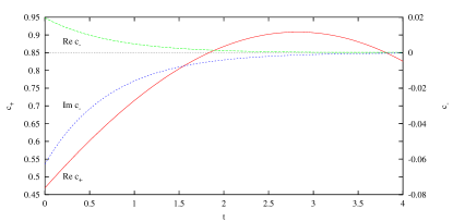
Figure 6: The large-time behavior of a solution with $\epsilon=0$ at $(E=1.05,\;N=0.43)$. The coordinates $X$ and $y$ are decomposed in the basis of the eigenmodes near the sphaleron. Note that $\mathop{\mathrm{Im}}c^{+}=0$.

III.2 Regularization technique versus exact quantum–mechanical solution

Quantum mechanics of two degrees of freedom is a convenient testing ground for checking the semiclassical methods and, in particular, our regularization technique. We have found the solutions to the full stationary Schrödinger equation and exact tunneling probability ${\cal T}$ by applying the numerical technique of Refs. Bonini:1999cn ; Bonini:1999kj . Our numerical calculations were performed for several small values of the semiclassical parameter $\lambda$, namely, for $\lambda=0.01$—$0.1$. Transitions through the barrier for these values of the semiclassical parameter are well suppressed. In particular, for $\lambda=0.02$ the tunneling probability ${\cal T}$ is of order $\mathrm{e}^{-14}$. To check the semiclassical result with better precision, we have calculated the exact suppression exponent $F_{\mathrm{QM}}(\lambda)\equiv-\lambda\log{\cal T}$ (cf. (5)) for $\lambda=0.09,0.05,0.03,0.02$ and extrapolated $F_{\mathrm{QM}}$ to $\lambda=0$ by polynomials of the third and fourth order. The results of extrapolation are independent of the order ($3$ or $4$) of polynomials with precision of $1\%$. The extrapolated suppression exponent $F_{\mathrm{QM}}(0)$ corresponds to infinite suppression and must exactly coincide (up to numerical errors) with the correct semiclassical result.

We performed this check in the region $E>E_{S}=1$, which is most interesting for our purposes. The results of the full quantum mechanical calculation of the suppression exponent $F_{\mathrm{QM}}$ in the limit $\lambda\to 0$ are represented by points in Fig. 7. The lines in that figure represent the values of the semiclassical exponent $F(E,N)$ for constant $N$, which we obtain in the limit $\epsilon\to 0$ of the regularization procedure. In practice, instead of taking the limit $\epsilon\to 0$ one calculates the regularized functional $F_{\epsilon}(E,N)=F(E,N)+O(\epsilon)$ for small enough $\epsilon$. In our calculations we used the value $\epsilon=10^{-6}$, so that the value of the suppression exponent was found with precision of order $10^{-5}$. We see that in the entire region of classically forbidden transitions (including the region $E>E_{1}(N)$) the semiclassical result for $F$ coincides with the exact one.

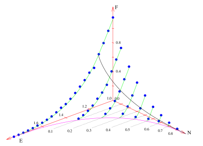
Figure 7: The tunneling exponent $F(E,N)$ in the region $E>E_{\mathrm{S}}=1$. The lines show the semiclassical results while points represent exact ones, obtained by solving the Schrödinger equation. The lines across the plot are the boundary of the region of classically allowed transitions $E_{0}(N)$ and the bifurcation line $E_{1}(N)$.

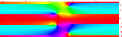
(a)

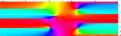
(b)

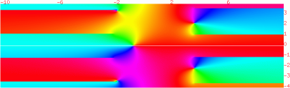
(c)

$\begin{array}[]{c}\pi\\ -\pi\end{array}\begin{array}[]{c}\includegraphics[width=28.45274pt]{fig18d}\end{array}0$

Figure 8: The phase of the tunneling coordinate in complex time plane at the three points of the curve $\tau=380$, $\vartheta=130$. Points (a), (b), (c) correspond to $\epsilon=\epsilon_{a}=0.01$, $\epsilon=\epsilon_{b}=0.0048$ and $\epsilon=\epsilon_{c}=0$, respectively. The asymptotics $X\to-\infty$ and $X\to+\infty$ correspond to $\mathrm{arg}(X)=\pi$ and $0$. The contour in the time plane is plotted with white line.

III.3 Classically allowed transitions

Let us show that our regularization procedure enables one to obtain a subset of classical over–barrier solutions, existing at high enough energies. This subset is interesting, as it extends all the way to the boundary of the region of classically allowed transitions, $E=E_{0}(N)$. In principle, finding this boundary is purely a problem of classical mechanics, and, indeed, in mechanics of two degrees of freedom one obtains this boundary numerically by solving the Cauchy problem for given $E$ and $N$ and all possible oscillator phases, see Sec. II.3. However, if the number of degrees of freedom is much larger, this classical problem becomes quite complicated, as one has to span a high-dimensional space of Cauchy data. As an example, a stochastic Monte Carlo technique was developed in Ref. Rebbi:1995zw to deal with this problem in field theory context. The approach below is as an alternative to the Cauchy methods.

First, let us recall that all classical over–barrier solutions with given energy and excitation number satisfy the $T/\theta$ boundary value problem with $T=0$, $\theta=0$. We cannot reach the “allowed” region of $E-N$ plane without regularization, since we have to cross the line $E_{0}(N)$ corresponding to the excited sphaleron configurations in the final state. However, the excited sphalerons are longer exist among the solutions of the regularized boundary value problem at any finite value of $\epsilon$. This suggests that the regularization enables one to enter the region of the classically allowed transitions and, after taking an appropriate limit, obtain classical solutions with finite values of $E$, $N$.

By definition, the classically allowed transitions have $F=0$. Thus, one expects that in the “allowed” region of initial data, the regularized problem has the property that $F_{\epsilon}(E,N)=\epsilon f(E,N)+O(\epsilon^{2})$. In view of the inverse Legendre formulas (12), (13) the values of $T$ and $\theta$ must be of order $\epsilon$: $T=\epsilon\tau(E,N)$, ${\theta=\epsilon\vartheta(E,N)}$, where the quantities $\tau$ and $\vartheta$ are related to the initial energy and excitation number (see Eqs. (12), (13)) in the following way,

$$\tau = -\lim\limits_{\epsilon\to 0}\frac{\partial}{\partial E}\frac{F_{\epsilon}}{\epsilon}=-\frac{1}{2}\frac{\partial}{\partial E}T_{\mathrm{int}}(E,N)\;,$$ (18)

$$\vartheta = -\lim\limits_{\epsilon\to 0}\frac{\partial}{\partial N}\frac{F_{\epsilon}}{\epsilon}=-\frac{1}{2}\frac{\partial}{\partial N}T_{\mathrm{int}}(E,N)\;,$$ (19)

where we have used Eq. (17). Therefore, one expects that one can invade the region of classically allowed transitions by taking a fairly sophisticated limit $\epsilon\to 0$ with $\tau\equiv T/\epsilon=\mathrm{const}$, $\vartheta\equiv\theta/\epsilon=\mathrm{const}$. For the allowed transitions the parameters $\tau$ and $\vartheta$ are analogous to $T$ and $\theta$.

By solving the regularized $T/\theta$ boundary value problem one constructs a single solution for given $E$ and $N$. On the other hand, for $\epsilon=0$ there are more classical over–barrier solutions: they form a continuous family labeled by the initial oscillator phase. Thus, after taking the limit $\epsilon\to 0$ one obtains a subset of over–barrier solutions, which should therefore obey some additional constraint. It is almost obvious, that this constraint is that the interaction time $T_{\mathrm{int}}$, Eq. (15), is minimal. This is shown in Appendix B.

The subset of classical over–barrier solutions obtained in the limit ${\epsilon\to 0}$ of the regularized $T/\theta$ procedure extends all the way to the boundary of the region of classically allowed transitions. Let us see what happens as one approaches this boundary from the “classically allowed” side. At the boundary $E_{0}(N)$, the unregularized solutions tend to excited sphalerons, so the interaction time $T_{\mathrm{int}}$ is infinite. This is consistent with (18), (19) only if $\tau$ and $\vartheta$ become infinite at the boundary. Thus, to obtain a point of the boundary one takes the further limit,

$$\big{(}E_{0}(N),\,N\big{)}=\lim_{\stackrel{{\scriptstyle\scriptstyle\tau/\vartheta=\mathrm{const}}}{{\scriptstyle\tau\to+\infty}}}\big{(}E(\tau,\vartheta),N(\tau,\vartheta)\big{)}\;.$$

Different values of $\tau/\vartheta$ correspond to different points of the line $E_{0}(N)$. In this way one finds the boundary of the region of classically allowed transitions without an initial-state simulation.

We have checked this procedure numerically. The limit $\epsilon\to 0$ exists indeed—the values of $E$ and $N$ tend to the point of the $E$–$N$ plane, which corresponds to the classically allowed transition. The phase of the tunneling coordinate $X(t)$ in complex time plane is shown in Fig. 8 for the three points (a), (b) and (c) of the curve $\tau\equiv T/\epsilon=380,\;\vartheta\equiv\theta/\epsilon=130$. Point (a) lies deep inside the tunneling region, $E_{a}<E_{1}(N_{a})$, point (c) corresponds to over-barrier solution with $T=0,\;\theta=0,\;\epsilon=0$, point (b) is in the middle of the curve. The branch points of the solution, the cuts and the contour are clearly seen on these graphs.

It is worth noting that the left branch points move down as $T$ and $\theta$ approach zero. Solutions close enough to the boundary $E_{0}(N)$ have left branch point in the lower complex half-plane, see Fig. 8. Therefore, the corresponding contour may be continuously deformed to the real time axis. These solutions still satisfy the reality conditions asymptotically (see Fig. 6), but show nontrivial complex behavior at any finite time.

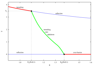
(a)

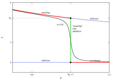
(b)

Figure 9: Dependence of the parameter $T=-\partial F/\partial E$ on energy for (a) two-dimensional model with fixed $N=0.1$ and (b) one-dimensional model (see Appendix C). Different lines correspond to different branches of classical solutions to $T/\theta$ boundary value problem. The branches labelled “reflection” end up on the wrong side of the barrier. Figure (b) contains also a line with nonzero $\epsilon$.

Making use of the regularized $T/\theta$ procedure, one is able to approach the boundary of the region of classically allowed transitions from both sides. The points at this boundary are obtained by taking the limits $T\to 0,\;T/\theta=\mathrm{const}$ of the tunneling solutions and $\tau\to+\infty$, ${\tau/\vartheta=\mathrm{const}}$ of the classically allowed ones. As $\tau^{*}\equiv\tau/\vartheta=T/\theta$ by construction, the lines $\tau^{*}=\mathrm{const}$ are continuous at the boundary $E_{0}(N)$, though may have discontinuity of the derivatives. The variable $\tau^{*}$ can be used to parametrize the curve $E_{0}(N)$.

IV Conclusions

We conclude that classical solutions describing transmissions of a bound system through a potential barrier with different values of energy and initial oscillator excitation number form three branches. These branches merge at bifurcation lines $E_{0}(N)$ and $E_{1}(N)$. Solutions from different branches describe physically different transition processes. Namely, solutions at low energies $E<E_{1}(N)$ describe conventional potential–like tunneling, while at $E>E_{0}(N)$ they correspond to unsuppressed over-barrier transitions. At intermediate energies, $E_{1}(N)<E<E_{0}(N)$, physically relevant solutions describe transitions on top of the barrier. This branch structure is shown in Fig. 9a, where the period $T=\partial F/\partial E$ obtained numerically for the solutions from different branches is plotted as function of energy for $N=0.1$.

One notices that the qualitative structure of branches in model, with internal degrees of freedom is similar to the structure of branches in one-dimensional quantum mechanics (see Appendix C). The latter is shown in Fig. 9b. The features of solutions in both cases are similar, though the solutions ending up on top of the barrier are degenerate in energy in one-dimensional case, and hence are not really physically interesting.

In this paper we introduced the regularization technique which enables one to connect smoothly solutions from different branches. Its advantage is that it automatically chooses the physically relevant branch. This technique is particularly convenient in numerical studies: we have seen that it enables one to cover the whole interesting region of parameter space. We applied this technique to baryon number violating processes in electroweak theoryBezrukov:2003er .

Appendix A $T/\theta$ boundary value problem

The semiclassical method for calculating the probability of tunneling from a state with a few parameters fixed was developed in Rubakov:1992ec ; Rubakov:1992fb ; Kuznetsov:1997az ; Bezrukov:2001dg in context of field theoretical models and in Miller:1970 ; Miller:1972 ; George:1972 ; Bonini:1999cn ; Bonini:1999kj in quantum mechanics. Here we outline the method, adapted to our model of two degrees of freedom.

A.1 Path integral representation of the transition probability

We begin with the path integral representation for the probability of tunneling from the asymptotic region $X\to-\infty$ through a potential barrier. Let the incoming state $|E,\;N\rangle$ have fixed energy and oscillator excitation number, and has support only for $X\ll 0$, well outside the range of the potential barrier. The inclusive tunneling probability for states of this type is given by

$$\mathcal{T}(E,N)=\lim\limits_{t_{f}-t_{i}\to\infty}\Bigg{\{}\int\limits_{0}^{+\infty}dX_{f}\int\limits_{-\infty}^{+\infty}dy_{f}\\ \left|\langle X_{f},y_{f}|\mathrm{e}^{-i\hat{H}(t_{f}-t_{i})}|E,N\rangle\right|^{2}\Bigg{\}}\;,$$ (20)

where $\hat{H}$ is the Hamiltonian operator. This probability can be reexpressed in terms of the transition amplitudes

$${\cal A}_{fi}=\langle X_{f},\;y_{f}|\mathrm{e}^{-i\hat{H}(t_{f}-t_{i})}|X_{i},\;y_{i}\rangle$$ (21)

and initial-state matrix elements

$${\cal B}_{ii^{\prime}}=\langle X_{i},\;y_{i}|E,\;N\rangle\langle E,\;N|X_{i}^{\prime},\;y_{i}^{\prime}\rangle$$ (22)

in the following way,

$${\cal T}(E,\;N)=\lim\limits_{t_{f}-t_{i}\to\infty}\Bigg{\{}\int\limits_{0}^{+\infty}dX_{f}\int\limits_{-\infty}^{0}d{X}_{i}\,d{X}_{i}^{\prime}\\ \int\limits_{-\infty}^{+\infty}dy_{i}\,dy_{i}^{\prime}\,dy_{f}\;{\cal A}_{fi}{\cal A}_{i^{\prime}f}^{*}{\cal B}_{ii^{\prime}}\Bigg{\}}\;.$$ (23)

The transition amplitude and its complex conjugate have the familiar path integral representation:

$$\mathcal{A}_{fi} = \int[d\vec{x}]\Bigg{|}_{\stackrel{{\scriptstyle\scriptscriptstyle\vec{x}(t_{i})=\vec{x}_{i}}}{{\scriptscriptstyle\vec{x}(t_{f})=\vec{x}_{f}}}}\mathrm{e}^{iS[\vec{x}]}\;,$$ (24)

$$\mathcal{A}_{i^{\prime}f}^{*} = \int[d\vec{x^{\prime}}]\Bigg{|}_{\stackrel{{\scriptstyle\scriptscriptstyle\vec{x}^{\prime}(t_{i})=\vec{x}^{\prime}_{i}}}{{\scriptscriptstyle\vec{x}^{\prime}(t_{f})=\vec{x}_{f}}}}\mathrm{e}^{-iS[\vec{x^{\prime}}]}\;,$$

where $\vec{x}=(X,y)$, and $S$ is the action of the model. To obtain a similar representation for the initial-state matrix elements, let us rewrite ${\cal B}_{ii^{\prime}}$ as follows,

$${\cal B}_{ii^{\prime}}=\langle X_{i},\;y_{i}|\hat{P}_{E}\hat{P}_{N}|X_{i}^{\prime},\;y_{i}^{\prime}\rangle\;,$$ (25)

where $\hat{P}_{N}$ and $\hat{P}_{E}$ denote the projectors onto states with oscillator excitation number $N$ and total energy $E$ respectively. It is convenient to use the coherent state formalism for the $y$-oscillator and choose the momentum basis for the $X$-coordinate. In this representation, the kernel of the projector operator $\hat{P}_{E}\hat{P}_{N}$ takes the form

$$\langle q,\;b|\hat{P}_{E}\hat{P}_{N}|p,\;a\rangle=\frac{1}{(2\pi)^{2}}\int d\xi\,d\eta\\ \mathrm{exp}\left(-iE\xi-iN\eta+\frac{i}{2}p^{2}\xi+\mathrm{e}^{i\omega\xi+i\eta}\bar{b}a\right)\delta(q-p)\;,$$

where $|p,\;a\rangle$ is the eigenstate of the center-of-mass momentum $\hat{p}_{X}$ and $y$-oscillator annihilation operator $\hat{a}$ with eigenvalues $p$ and $a$ respectively. It is straightforward to express this matrix element in the coordinate representation using the formulas

$$\langle y|a\rangle = \sqrt[4]{\frac{\omega}{\pi}}\mathrm{e}^{-\frac{1}{2}a^{2}+\sqrt{2\omega}ay-\frac{1}{2}\omega y^{2}}\;,$$

$$\langle X|p\rangle = \frac{1}{\sqrt{2\pi}}\mathrm{e}^{ipX}\;.$$

Evaluating the Gaussian integrals over $a$, $b$, $p$, $q$, we obtain

$${\cal B}_{ii^{\prime}} = \int d\xi\;d\eta\;\mathrm{exp}\left(-iE\xi-iN\eta-\frac{i}{2}\frac{(X_{i}-X_{i}^{\prime})^{2}}{\xi}\right.$$ (26)

$$+\left.\frac{\omega}{1-\mathrm{e}^{-2i\omega\xi-2i\eta}}\left[\frac{y_{i}^{2}+y_{i}^{\prime 2}}{2}(1+\mathrm{e}^{-2i\omega\xi-2i\eta})\right.\right.$$

$$\quad\quad\quad\quad\quad\quad\quad\quad\quad-2y_{i}y_{i}^{\prime}\mathrm{e}^{-i\omega\xi-i\eta}\bigg{]}\bigg{)}$$

where we omit the pre-exponential factor depending on $\eta,\;\xi$. For the subsequent formulation of the boundary value problem it is convenient to introduce the notations

$$T=-i\xi\;,\qquad\theta=-i\eta\;.$$

Then, combining together the integral representations (26) and (24) and rescaling coordinates, energy and excitation number $\vec{x}\to\vec{x}/\sqrt{\lambda}$, $E\to E/\lambda$, $N\to N/\lambda$, we finally obtain

$${\cal T}(E,\;N)=\lim\limits_{t_{f}-t_{i}\to\infty}\Bigg{\{}\int\limits_{-i\infty}^{+i\infty}dT\;d\theta\int\;[d\vec{x}\;d\vec{x}^{\prime}]\\ \exp\left\{-\frac{1}{\lambda}F[\vec{x},\;\vec{x}^{\prime};\;T,\;\theta]\right\}\Bigg{\}}\;,$$ (27)

where

$$F[\vec{x},\;\vec{x}^{\prime};\;T,\;\theta]=-iS[X,y]+iS[X^{\prime},\;y^{\prime}]\\ -ET-N\theta+B_{i}(\vec{x}_{i},\vec{x^{\prime}}_{i};T,\theta).$$ (28)

Here the non-trivial initial term $B_{i}$ is

$$B_{i}=\Bigg{\{} \frac{(X_{i}-X_{i}^{\prime})^{2}}{2T}$$

$$-\frac{\omega}{1-\mathrm{e}^{2\omega T+2\theta}}\bigg{[}\frac{1}{2}(y_{i}^{2}+{y_{i}^{\prime}}^{2})(1+\mathrm{e}^{2\omega T+2\theta})$$

$$\hphantom{-\frac{\omega}{1-\mathrm{e}^{2\omega T+2\theta}}\bigg{[}}-2y_{i}y_{i}^{\prime}\mathrm{e}^{\omega T+\theta}\bigg{]}\Bigg{\}}.$$ (29)

In (27) $\vec{x}$ and $\vec{x^{\prime}}$ are independent integration variables, while $\vec{x}_{f}^{\prime}\equiv\vec{x}_{f}$, see Eqs. (23).

A.2 The boundary value problem

For small $\lambda$, the path integral (27) is dominated by a stationary point of the functional $F$. Thus, to calculate the tunneling probability exponent, we extremize this functional with respect to all variables of integration: $X(t)$, $y(t)$, $X^{\prime}(t)$, $y^{\prime}(t)$, $T$, $\theta$. Note that because of the limit $t_{f}-t_{i}\to+\infty$, the variation with respect to the initial and final values of coordinates leads to boundary conditions imposed at asymptotic $t\to\pm\infty$, rather than at finite times $t_{i},t_{f}$. Note also that the stationary points may be complex.

The variation of the functional (28) with respect to the coordinates at intermediate times gives second order equations of motion, in general complexified,

$$\frac{\delta S}{\delta X(t)}=\frac{\delta S}{\delta y(t)}=\frac{\delta S^{\prime}}{\delta X^{\prime}(t)}=\frac{\delta S^{\prime}}{\delta y^{\prime}(t)}=0\;.$$ (30a)

The boundary conditions at the final time $$t_{f}\to+\infty F X_{f}\equiv X_{f}^{\prime} y_{f}\equiv y_{f}^{\prime}$$ are obtained by extremization of with respect to , . These are

$$\dot{X_{f}}=\dot{X_{f}^{\prime}}\;,\qquad\dot{y_{f}}=\dot{y_{f}^{\prime}}\;.$$ (30b)

It is convenient to write the conditions at the initial time (obtained by varying $$X_{i} y_{i} X_{i}^{\prime} y_{i}^{\prime} t_{i}\to-\infty X\to-\infty$$, , , ) in terms of the asymptotic quantities. At the initial moment of time , the system moves in the region , well outside of the range of the potential barrier. Equations (30a) in this region describe free motion of decoupled oscillator, and the general solution takes the following form,

$$X(t)=X_{i}+p_{i}(t-t_{i}),$$

$$y(t)=\frac{1}{\sqrt{2\omega}}\left[a\mathrm{e}^{-i\omega(t-t_{i})}+\bar{a}\mathrm{e}^{i\omega(t-t_{i})}\right]\;,$$

while the solution for $$X^{\prime}(t) y^{\prime}(t) a \bar{a} X_{i} p_{i} a \bar{a}$$, has similar form. For the moment, and are independent variables. The initial boundary conditions in terms of the asymptotic variables , , , take the form:

$$p_{i}=p_{i}^{\prime}=-\frac{X_{i}-X_{i}^{\prime}}{iT},$$

$$a^{\prime}+\bar{a}^{\prime}=a\mathrm{e}^{\omega T+\theta}+\bar{a}\mathrm{e}^{-\omega T-\theta}\;,$$ (30c)

$$a+\bar{a}=a^{\prime}\mathrm{e}^{-\omega T-\theta}+\bar{a}^{\prime}\mathrm{e}^{\omega T+\theta}\;.$$

The variation with respect to the Lagrange multipliers $$T \theta E N$$ and gives the relation between the values of , and initial asymptotic variables (here we use the boundary conditions (30c)),

$$E = \frac{p_{i}^{2}}{2}+\omega N\;,$$ (30d)

$$N = a\bar{a}\;.$$

Equations (30a) – (30d) constitute the complete set of saddle-point equations for the functional $$F$$.

The variables $X^{\prime}$ and $y^{\prime}$ originate from the conjugate amplitude ${\cal A}_{i^{\prime}f}^{*}$ (see Eq. (24)), which suggests that they are the complex conjugate to $X$, $y$. Indeed, the Ansatz ${X^{\prime}(t)=X^{*}(t)}$, ${y^{\prime}(t)=y^{*}(t)}$ is compatible with the boundary value problem (30). Then the Lagrange multipliers $T$, $\theta$ are real, and the problem (30) may be conveniently formulated at the contour ABCD in the complex time plane (see Fig. 2).

Now we have only two independent complex variables $X(t)$ and $y(t)$, that have to satisfy the classical equations of motion in the interior of the contour,

$$\frac{\delta S}{\delta X(t)}=\frac{\delta S}{\delta y(t)}=0\;.$$ (31a)

The final boundary conditions (see Eq. (30b)) become the conditions of the reality of the variables $$X(t) y(t)$$ and at the asymptotic part D of the contour:

$$\begin{array}[]{l}\mathop{\mathrm{Im}}X_{f}=0,\;\;\mathop{\mathrm{Im}}y_{f}=0\;,\\[4.30554pt] \mathop{\mathrm{Im}}\dot{X}_{f}=0\;\;\mathop{\mathrm{Im}}\dot{y}_{f}=0\;,\end{array}\qquad t\to+\infty\;.$$ (31d)

The seemingly complicated initial conditions (30c) simplify when written in terms of the time coordinate $$t^{\prime}=t+iT/2$$ running along the part AB of the contour. Let us again write the asymptotics of a solution, but now along the initial part AB of the contour:

$$X=X_{0}+p_{0}(t^{\prime}-t_{i})\;,$$

$$y=\frac{1}{\sqrt{2\omega}}\left[u\mathrm{e}^{-i\omega(t^{\prime}-t_{i})}+v\mathrm{e}^{i\omega(t^{\prime}-t_{i})}\right]\;.$$

In terms of $$X_{0} y_{0} u v$$, , and , the boundary conditions (30c) are

$$\mathop{\mathrm{Im}}X_{0}=0,\;\;\mathop{\mathrm{Im}}p_{0}=0\;,$$ (31e)

$$v=u^{*}\mathrm{e}^{\theta}\;.$$

Finally, we write Eqs. (30d) in terms of the asymptotic variables along the initial part of the contour:

$$E=\frac{p_{0}^{2}}{2}+\omega N\;,$$ (32)

$$N=\omega uv\;.$$

These equations determine the Lagrange multipliers $T,\;\theta$ in terms of $E$, $N$. Alternatively, we can solve the problem (31) for given values of $T$, $\theta$ and find the values of $E$,$N$ from Eqs. (32), what is more convenient computationally.

Given a solution to the problem (31), the exponent $F$ is the value of the functional (28) at this saddle point. In this way we obtain the expression (8) for the tunneling exponent. The exponent $F$ is expressed now in terms of $S_{0}$, eq. (9) — integrated by parts action of the system. Non–trivial boundary term $B_{i}$, eq. (A.1), is cancelled by the boundary term coming from the integration by parts. Note that we did not make use of the constraints (32) to obtain the formula (8), so we still have to extremize (8) with respect to $T$ and $\theta$ (see discussion in Sec. II.2).

The classical problem (31) is conveniently dubbed $T/\theta$ boundary value problem. Eqs. (31d) and (31e) imply eight real boundary conditions for two complex second-order differential equations (31a). However, one of these real conditions is redundant: Eq. (31d) implies that the (conserved) energy is real, so the condition $\mathop{\mathrm{Im}}p_{0}\to 0$ is automatically satisfied (note that the oscillator energy $E_{\mathrm{osc}}=\omega uv=\omega\mathrm{e}^{\theta}uu^{*}$ is real). On the other hand, the system (31) is invariant under time translations along the real axis. This invariance is fixed, e.g., by demanding that $\mathop{\mathrm{Re}}(X)$ takes a prescribed value at a prescribed large negative time $t^{\prime}_{0}$ (note that other ways may be used instead. In particular, for $E<E_{1}(N)$ it is convenient to impose the constraint $\mathop{\mathrm{Re}}\dot{X}({t=0})=0$). Together with the latter requirement, we have exactly eight real boundary conditions for the system of two complexified (i.e. four real) second-order equations.

Appendix B A property of solutions to $T/\theta$ problem in for the case of over–barrier transitions

For given $E$, $N$ there is only one over–barrier classical solution which is obtained in the limit $\epsilon\to 0$ of the regularized $T/\theta$ procedure. To see what singles out this solution, let us analyze the regularized functional

$$F_{\epsilon}[q]=F[q]+2\epsilon T_{\mathrm{int}}[q],$$ (33)

where $q$ denotes the variables $\vec{x}(t),\;\vec{x}^{\prime}(t)$ and $T,\;\theta$ together. The unregularized functional $F$ has a valley of extrema $q^{e}(\varphi)$ corresponding to different values of the initial oscillator phase $\varphi$. Clearly, at small $\epsilon$ the extremum of $F_{\epsilon}$ is close to a point in this valley with the phase extremizing $T_{\mathrm{int}}[q^{e}(\varphi)]$.

$$\frac{d}{d\varphi}T_{\mathrm{int}}[q^{e}(\varphi)]=0\;.$$ (34)

Hence, the solution $q^{e}_{\epsilon}$ of the regularized $T/\theta$ boundary value problem tends to the over–barrier classical solution, with $T_{\mathrm{int}}$ extremized with respect to the initial oscillator phase.

Because $U_{\mathrm{int}}(\vec{x})>0$, $T_{\mathrm{int}}$ is a positive quantity with at least one minimum. In normal situation there is only one saddle point of $F_{\epsilon}$, so by solving the $T/\theta$ boundary value problem one obtains the classical solution with the time of interaction minimized.

Appendix C Classically allowed transitions: one-dimensional example

The difficulties with bifurcations of classical solutions emerge in quite a general class of quantum mechanical models. To illustrate this statement, let us consider the case of one-dimensional quantum mechanics, where the result is given by well-known WKB formula. We will show that the origin of the above difficulties can be seen in one-dimensional model also. The implementation of the regularization technique is explicit in one dimensional case. This makes it easy to see how our technique allows one to join smoothly classical solutions relevant to the tunneling and allowed transitions.

In quantum mechanics of one degree of freedom only one variable $X(t)$ is present, which describes motion of a particle with mass $m=1$ through a potential barrier $U(X)$. The motion is free in the asymptotic regions $X\to\pm\infty$. The semiclassical calculation of the tunneling exponent is performed by solving the classical equation of motion

$$\frac{\delta S}{\delta X(t)}=0$$

on the contour ABCD in complex time plane, with the conditions that the solution is real in the asymptotic past (region A), and asymptotic future (region D). The relevant solutions tend to $X\to-\infty$ and $X\to+\infty$ in regions A and D, respectively. The auxiliary parameter $T$ is related to the energy of incoming state by the requirement that the energy of the classical solution equals to $E$. The exponent for the transition probability is

$$F=2\mathop{\mathrm{Im}}S-ET\;.$$ (35)

One notes the resemblance of these boundary conditions to the ones on the tunneling coordinate $X$ in two-dimensional system.

In quantum mechanics of one degree of freedom, the contour ABCD may be chosen in such a way that the points B and C are the turning points of the solution. Then the solution is real also at the part BC of the contour. Indeed, a real solution at the part BC of the contour oscillates in the upside-down potential, $T/2$ equals to half-period of oscillations, and the points B and C are the two different turning points, $\dot{X}=0$. The continuation of this solution, according to the equation of motion, from the point C to the positive real times corresponds to the real-time motion, with zero initial velocity, towards $X\to+\infty$; the coordinate $X(t)$ stays real on the part CD of the contour. Likewise, the continuation back in time from the point B leads to real solution in the part AB of the contour. In this way the reality conditions are satisfied at A and D. The only contribution to $F$ comes from the Euclidean part of the contour, and one can check that the expression (35) reduces to

$$F(E)=2\int\limits_{X_{B}}^{X_{C}}\!\sqrt{2(U(X)-E)}\,dX\;,$$ (36)

which is the standard WKB result.

The solutions appropriate for the classically forbidden and classically allowed transitions apparently belong to different branches. As the energy approaches the height of the barrier $U_{0}$ from below, the amplitude of the oscillations in the upside-down potential decreases, while the period $T$ tends to a finite value determined by the curvature of the potential at its maximum. On the other hand, the solutions for $E>U_{0}$ always run along the real time axis, so the parameter $T$ is always zero. Hence, the relevant solutions do not merge at $E=U_{0}$, and $T(E)$ has a discontinuity at $E=U_{0}$. The regularization technique of Sec. III.1 removes this discontinuity and allows for smooth transitions through the point $E=U_{0}$. The only difference with quantum mechanics of multiple degrees of freedom is that in the latter case the bifurcation points exist not only at the boundary of the region of classically allowed transitions, but also well inside the region of classically forbidden transitions (but still at $E>E_{S}$, see Introduction and Sec. II.3).

To illustrate the situation, let us consider an exactly solvable model with

$$U(X)=\frac{1}{\cosh^{2}X}\;.$$

We implement our regularization technique by formally changing the potential

$$U(X)\to\mathrm{e}^{-i\epsilon}U(X)\;,$$ (37)

which leads to the corresponding change of the classical equations of motion. Here $\epsilon$ is a real regularization parameter, the smallest parameter in the model. At the end of the calculations one takes the limit $\epsilon\to 0$.

We do not change the boundary conditions in our regularized classical problem, i.e., we still require that $X(t)$ be real in the asymptotic future on the real time axis and that $X(t^{\prime})$ be real as $t^{\prime}\to-\infty$ on the part A of the contour ABCD. Then the conserved energy is real. The sphaleron solution $X(t)=0$ has now complex energy (because the potential is complex). Hence, the solutions to our classical boundary value problem necessarily avoid the sphaleron, and one may expect that the solutions behave smoothly in energy.

The general solution to the regularized problem is

$$\sqrt{\frac{E}{\mathrm{e}^{-i\epsilon}-E}}\sinh X=-\cosh\left(\sqrt{2E}(t-t_{0})\right)\;,$$

where $t_{0}$ is the integration constant. The value of $\mathop{\mathrm{Im}}t_{0}$ is fixed by the requirement that $\mathop{\mathrm{Im}}X=0$ at positive time $t\to+\infty$,

$$\mathop{\mathrm{Im}}t_{0}=\frac{T}{2}-\frac{1}{2\sqrt{2E}}\mathrm{arg}[\mathrm{e}^{-i\epsilon}-E]\;.$$

The residual parameter $\mathop{\mathrm{Re}}t_{0}$ represents the real–time translational invariance present in the problem. The condition that the coordinate $X$ is real on the initial part AB of the contour gives the relation between $T$ and $E$,

$$\frac{T}{2}=\frac{1}{\sqrt{2E}}\left\{\pi+\arg\left(\mathrm{e}^{-i\epsilon}-E\right)\right\}\;.$$ (38)

For $\epsilon=0$ and $E<1$, the original unregularized result $T/2=\pi/\sqrt{2E}$ is reproduced.

Let us analyze what happens in the regularized case in the vicinity of the would-be special value of energy, $E=E_{\mathrm{S}}\equiv 1$. It is clear from Eq. (38) that T is now a smooth function of $E$. Away from $E=1$, Eq. (38) can be written as follows,

$$\frac{T}{2}=\left\{\begin{array}[]{ll}\displaystyle\frac{\pi}{\sqrt{2E}}&\text{forbidden region, }1-E\gg\epsilon\\ \displaystyle\frac{\epsilon}{\sqrt{2E}(E-1)}&\text{allowed region, }E-1\gg\epsilon.\end{array}\right.$$ (39)

Deep enough in the region of forbidden transitions, when $1-E\gg\epsilon$, the argument in equation (38) is nearly zero and we return to the original tunneling solution. When $E$ crosses the region of size of order $\epsilon$ around $E=1$, the argument rapidly changes from $O(\epsilon)$ to $-\pi$, so that $T/2$ changes from $\pi/\sqrt{2}$ to nearly zero. Thus, at $E>1$ we arrive to a solution which is very close to the classical over-barrier transition, and the contour is also very close to the real axis. This is shown in Fig. 9. We conclude that at small but finite $\epsilon$, the classically allowed and classically forbidden transitions merge smoothly.

At ${E<1}$, the limit $\epsilon\to 0$ is straightforward. For ${E>1}$ a somewhat more careful analysis of the limit ${\epsilon\to 0}$ is needed. From Eq. (39) one observes that the limit ${\epsilon\to 0}$ with constant finite $T<\pi\sqrt{2}$ leads to solutions with $E=1$. Classical over-barrier solutions of the original problem with $E>E_{S}\equiv 1$ are obtained in the limit $\epsilon\to 0$ provided that $T$ also tends to zero while $\tau=T/\epsilon$ is kept finite. Different energies correspond to different values of $\tau$. And that is what one expects—classical over–barrier transitions are described by the solutions on the contour with $T\equiv 0$.

References

- (1) Z. Huang, T. Feuchtwang, P. Cutler and E. Kazes, Phys. Rev. A 41, 32 (1990).
- (2) S. Takada and H. Nakamura, J. Chem. Phys. 100, 98 (1994).
- (3) W. Miller, J. Chem. Phys. 53, 3578 (1970).
- (4) W. Miller and T. George, J. Chem. Phys. 56, 5668 (1972).
- (5) T. George and W. Miller, J. Chem. Phys. 57, 2458 (1972).
- (6) W. H. Miller, Adv. Chem. Phys. 25, 69 (1974).
- (7) M. Wilkinson, Physica 21D, 341 (1986).
- (8) M. Wilkinson and J. Hannay, Physica 27D, 201 (1987).
- (9) S. Takada, P. Walker and M. Wilkinson, J. Chem. Phys. 52, 3546 (1995).
- (10) S. Takada, J. Chem. Phys. 104, 3742 (1996).
- (11) G. F. Bonini, A. G. Cohen, C. Rebbi and V. A. Rubakov, quant-ph/9901062.
- (12) G. F. Bonini, A. G. Cohen, C. Rebbi and V. A. Rubakov, Phys. Rev. D60, 076004 (1999), [hep-ph/9901226].
- (13) V. A. Rubakov, D. T. Son and P. G. Tinyakov, Phys. Lett. B287, 342 (1992).
- (14) A. N. Kuznetsov and P. G. Tinyakov, Phys. Rev. D56, 1156 (1997), [hep-ph/9703256].
- (15) F. Bezrukov, C. Rebbi, V. Rubakov and P. Tinyakov, hep-ph/0110109.
- (16) F. Bezrukov, D. Levkov, C. Rebbi, V. Rubakov and P. Tinyakov, Phys. Rev. D68, 036005 (2003), [hep-ph/0304180].
- (17) A. M. Perelomov, V. S. Popov and M. V. Terent’ev, ZHETF 51, 309 (1966).
- (18) V. S. Popov, V. Kuznetsov and A. M. Perelomov, ZHETF 53, 331 (1967).
- (19) N. Makri and W. Miller, J. Chem. Phys. 89, 2170 (1988).
- (20) K. Thompson and N. Makri, J.Chem.Phys. 110, 1343 (1999).
- (21) K. Kay, J.Chem.Phys. 107, 2313 (1997).
- (22) N. Maitra and E. Heller, Phys.Rev.Lett. 78, 3035 (1997).
- (23) W. Miller, J. Phys. Chem. A 105, 2942 (2001).
- (24) A. N. Kuznetsov and P. G. Tinyakov, Mod. Phys. Lett. A11, 479 (1996), [hep-ph/9510310].
- (25) M. Davis and E. Heller, J.Chem.Phys. 75, 246 (1981).
- (26) E. Heller and M. Davis, J.Phys.Chem. 85, 309 (1981).
- (27) E. Heller, J.Phys.Chem. 99, 2625 (1994).
- (28) T. Banks, G. Farrar, M. Dine, D. Karabali and B. Sakita, Nucl. Phys. B347, 581 (1990).
- (29) V. I. Zakharov, Phys. Rev. Lett. 67, 3650 (1991).
- (30) G. Veneziano, Mod. Phys. Lett. A7, 1661 (1992).
- (31) V. A. Rubakov, hep-ph/9511236.
- (32) V. A. Rubakov and P. G. Tinyakov, Phys. Lett. B279, 165 (1992).
- (33) F. R. Klinkhamer and N. S. Manton, Phys. Rev. D30, 2212 (1984).
- (34) S. Y. Khlebnikov, V. A. Rubakov and P. G. Tinyakov, Nucl. Phys. B367, 334 (1991).
- (35) C. Rebbi and R. Singleton, hep-ph/9502370.