Quantum signatures of breather-breather interactions

Abstract

The spectrum of the Quantum Discrete Nonlinear Schrödinger equation on a periodic 1D lattice shows some interesting detailed band structure which may be interpreted as the quantum signature of a two-breather interaction in the classical case. We show that this fine structure can be interpreted using degenerate perturbation theory.

I Introduction

The localization and transport of energy in lattices by intrinsic localized modes or discrete breathers, has recently been the subject of intense theoretical and experimental investigation ( see Vázquez et al. (2003) and references therein). Corresponding results on the quantum equivalent of these states are less numerous, c.f.  Scott et al. (1994); MacKay (2000) for some theoretical results and Fillaux et al. (1998) for some experimental work. Studies of quantum modes on small lattices are of increasing interest for quantum devices based on quantum dots (c.f. Li et al. (2003)) and for studies of photonic crystals.

We present some results on breather bands in small one dimensional lattices with a small number of quanta. We study a periodic lattice with $f$ sites containing bosons, described by the quantum version of the discrete nonlinear Schrödinger equation (DNLS) which will be denoted by QDNLS. It has the Hamiltonian

$$H_{1}=-\sum_{s=1}^{f}\left[\gamma_{1}a_{s}^{\dagger}a_{s}^{\dagger}a_{s}a_{s}+\epsilon a_{s+1}^{\dagger}a_{s}+\text{h.c.}\right],$$ (1)

which conserves the number of quanta $n$. This model, also known as the Bose-Hubbard model, is presently used to investigate cold bosonic atoms in optical lattices Jaksch98 .

Assuming that the anharmonic parameter $\gamma_{1}>0$ is stronger than the intersite coupling, the eigenvalues of (1), plotted as a function of the wave number $k$, separate out into distinct bands Scott et al. (1994). The eigenstates of each band are dominated by states in which the bosons have clumped together, two or more on one site. For example, with $n=4$, the lowest band is, to a good approximation, a linear combination of states with 4 bosons on site $i$ and no bosons elsewhere. The next lowest band is mostly composed of states with 3 quanta on one site and another quanta elsewhere. The third band is mostly composed of states with 2 quanta on one site and 2 quanta on a separate site. We will refer to this band as a $\{2,2\}$ band in an obvious notation. This band is of great interest since it represents the simplest case of a band describing two “composite” particles interacting with each other. Our letter is devoted to the fine structure of this and similar bands such as the $\{4,2\}$ and $\{3,3\}$ bands in the $n=6$ case.

The fine structure of the $\{2,2\}$ band, see Fig. 1, shows the eigenvalues (crosses) in the $n=4$ case.

Figure 1: Detail of the eigenvalue spectrum for the QDNLS periodic lattice (1), $n=4,f=19,\gamma_{1}=10,\epsilon=0.5$.

The solid lines show the results of the theoretical calculations (described below) in the asymptotic limit $f\rightarrow\infty$. We stress again that this picture shows only one of the bands in the $n=4$ spectrum. Its fine detail is revealed as a “continuum” band (in the $f\rightarrow\infty$ limit), plus a single $k$-dependent “line band”. Examination of the corresponding eigenvectors shows that the “line band” is mostly composed of states where the two sites each with two quanta lie occupy adjacent sites, whereas in the “continuum” band these sites are separated by one or more vacant sites.

II Generalized Hamiltonian

The standard QDNLS Hamiltonian is thermodynamically unstable, i.e. the energy of the ground state goes to $-\infty$ as the number of particles goes to $+\infty$. Moreover, some bands can be degenerate with others, for example when $n=6$, the $\{3,3\}$ band overlaps with the $\{4,1,1\}$ band. In some cases it would be convenient for the bands under study to be the lowest energy bands of the system.

For these reasons we consider also the following generalized QDNLS Hamiltonian

$$H_{2}=H_{1}+\gamma_{2}\sum_{s=1}^{f}a_{s}^{\dagger}a_{s}^{\dagger}a_{s}^{\dagger}a_{s}a_{s}a_{s}\,.$$ (2)

The $\gamma_{2}>0$ term is a saturation term which discourages too many bosons occupying the same site. A similar term appears also in nonlinear optics Michinel et al. (2002) and in cold bosonic atoms trapped in optical lattices gammal00 where it describes three body interactions. By varying the values of $\gamma_{1}$ and $\gamma_{2}$ it is possible to “shuffle” the order of bands in the $(E,k)$ diagram.

At zero coupling ($\epsilon=0$), we denote by $E_{s}$ the respective energies of $s$ bosons on the same site, $E_{1}=0,\quad E_{2}=-2\gamma_{1},\quad E_{3}=-6(\gamma_{1}-\gamma_{2}),\quad E_{4}=-12(\gamma_{1}-2\gamma_{2})$, etc. Thus in the $n=4$ case the $\{4\}$ band has energy $E_{4}$, the $\{31\}$ band has energy $E_{3}$, the $\{22\}$ band energy $2E_{2}$, etc. Providing $\gamma_{1}<3\gamma_{2}$, the bottom of the $\{22\}$ band is the ground state of the system.

III Perturbation Theory

To describe the components of the quantum states we use a position state representation, where for example the state $|020020\dots\rangle$ represents a state with two quanta at the lattice position 2, two quanta at the lattice position 5, and zero quanta elsewhere. In view of the periodic nature of the lattice, we can generate an equivalence class of states by applying the translation operator (with periodic boundary condition) to one of these states. We will refer to these classes by ordering them such that the leftmost number is the largest, so for example $|3000\dots\rangle$ is shorthand for $|3000\dots\rangle,|0300\dots\rangle,|0030\dots\rangle$, etc. For further conciseness we will truncate all trailing zeros, so the above class becomes $|3\rangle$. The set of all the classes containing $|22\rangle,|202\rangle,|2002\rangle$, etc. is referred to as the $\{2,2\}$ band.

At zero coupling, all the $\{2,2\}$ states $|22\rangle$, $|202\rangle,|2002\rangle,\dots$ are degenerate. We use degenerate perturbation theory to obtain both eigenvalues and eigenstates for $\epsilon\neq 0$. For the sake of simplicity, we consider an odd number of sites $f=2\sigma+1$. Bloch waves of $\{2,2\}$ states can be written (in the notation of Scott (2003))

$$|\psi\rangle=\sum_{j=1}^{\sigma}c_{j}|\psi_{j}\rangle$$ (3)

where

$$|\psi_{j}\rangle=\frac{1}{\sqrt{f}}\sum_{s=1}^{f}(\hat{T}/\tau)^{s-1}|2,\underbrace{0,\dots,0}_{j-1},2\rangle$$ (4)

Here $\hat{T}$ is the translation operator, $\tau=e^{ik}$, and the crystal momentum $k=2\pi l/f$ where $l\in\{-\sigma,\dots,\sigma\}$.

Using (3) and standard Brillouin-Wigner perturbation theory up to second order in $\epsilon$ we obtain

$$(E-2E_{2})c_{j} =\sum_{j^{\prime}=1}^{\sigma}\langle\psi_{j}|V|\psi_{j^{\prime}}\rangle c_{j^{\prime}}+$$ (5)

$$\quad+\sum_{j^{\prime}=1}^{\sigma}\sum_{\tilde{\psi}}\frac{\langle\psi_{j}|V|\tilde{\psi}\rangle\langle\tilde{\psi}|V|\psi_{j^{\prime}}\rangle}{2E_{2}-\tilde{E}}c_{j^{\prime}}$$

where $V$ is the hopping term in the Hamiltonian, and $|\tilde{\psi}\rangle$ is any state not in the $\{2,2\}$ subspace. $\tilde{E}$ is the energy corresponding to $|\tilde{\psi}\rangle$ in the uncoupled limit ($\epsilon=0$).

It is obvious that the first sum of (5) is zero as $V$ does not link any of the $|\psi_{s}\rangle$ to each other. In evaluating the second sum, the $\langle\cdot|V|\cdot\rangle$ terms are mostly zero except for the following

$$\langle 22|V|112\rangle=e^{ik}\surd 2\epsilon=e^{ik}\langle 22|V|211\rangle,$$

$$\langle 22|V|13\rangle=\surd 6\epsilon=\langle 22|V|31\rangle,$$

$$\langle 202|V|112\rangle=\surd 2\epsilon=\langle 202|V|211\rangle,$$

$$\langle 202|V|1102\rangle=e^{ik}\surd 2\epsilon=e^{ik}\langle 202|V|2011\rangle,\,\dots$$

We now define the matrix $H^{(22)}_{j,j^{\prime}}$ by

$$H^{(22)}_{j,j^{\prime}}=\sum_{\tilde{\psi}}\frac{\langle\psi_{j}|V|\tilde{\psi}\rangle\langle\tilde{\psi}|V|\psi_{j^{\prime}}\rangle}{2E_{2}-\tilde{E}}\,.$$ (6)

Then

$$H^{(22)}=\frac{8\epsilon^{2}}{E_{2}-2E_{1}}\,I_{\sigma}+\frac{4\epsilon^{2}}{E_{2}-2E_{1}}\left(\begin{array}[]{ccccc}\Gamma&\kappa^{*}&&&\\ \kappa&0&\kappa^{*}&&\\ &\ddots&\ddots&\ddots&\\ &&\kappa&0&\kappa^{*}\\ &&&\kappa&p\end{array}\right)$$ (7)

where $I_{m}$ is the $m\times m$ unity matrix and

$$\Gamma = \frac{3(E_{2}-2E_{1})}{2E_{2}-E_{3}-E_{1}}-1=\frac{3\gamma_{2}-4\gamma_{1}}{\gamma_{1}-3\gamma_{2}}\,,$$ (8)

$$\kappa = e^{i\frac{k}{2}}\cos\left(\frac{k}{2}\right)\ \text{and}\ p=\cos\sigma k\,.$$ (9)

The structure of the matrix (7) is very similar to the two-quanta case described in Scott et al. (1994). The first term represents a global shift of the $\{2,2\}$-band, whereas the “impurity” $\Gamma$ will in general be responsible for a splitting of the states $|22\rangle$ from the rest of the band ($|202\rangle$, $|2002\rangle$, etc.). In this respect, the $|22\rangle$’s can be seen as “bound states of doublets” within the $\{2,2\}$-band. It is separated from the continuum band because in addition to linking with states such as $|211\rangle$, it also links to states such as $|31\rangle$. This explains the $\{2,2\}$-band fine structure.

In case the number of sites tends to infinity, (7) may be diagonalised exactly to yield

$$E=2E_{2}+\left\{\!\begin{array}[]{c}\frac{4\epsilon^{2}}{E_{2}-2E_{1}}\left(2+\Gamma+\frac{\cos^{2}(k/2)}{\Gamma}\right)\ \text{iff}\ |\Gamma|>\cos\left(\frac{k}{2}\right)\\ \\ \frac{8\epsilon^{2}}{E_{2}-2E_{1}}\left(1+\cos\left(\frac{k}{2}\right)\cos\theta\right)\ \text{where}\ \theta\in(0,\pi)\end{array}\right.$$ (10)

Depending on the various values of $\gamma_{1},\gamma_{2}$, and $\epsilon$, we can get the line band completely above or below the continuum band, or partially merged with the continuum band.

Figure 2: Detail of the eigenvalue spectrum for the generalized QDNLS periodic lattice (2), $n=4,f=19,\gamma_{1}=10,\gamma_{2}=7.5,\epsilon=0.5$.

Fig 2 shows a case where the line part is below the continuum part of the $\{2,2\}$ band and represents the ground state of the $n=4$ sector.

To provide some insight in the way the two groups of two quanta interact within a $|22\rangle$ state, we compare its effective mass $m_{22}^{*}$ with twice the effective mass $m_{2}^{*}$ of a single $|2\rangle$ state. From Scott et al. (1994) and (10), we obtain $m_{2}^{*}\simeq\gamma_{1}/(2\epsilon^{2})$ as $\epsilon\rightarrow 0$ and $m_{22}^{*}/(2m_{2}^{*})=\Gamma$ (see (8)). Depending on the ratio $\gamma_{2}/\gamma_{1}$, $\Gamma$ and thus $m_{22}^{*}$ are either positive or negative. The same phenomenon is observed for bright solitons in systems of Bose-Einstein condensates in optical lattices for which (1) may be seen as a tight-binding limit (see Mar03 and references therein).

IV The $n=6$ case

As a further example we consider the $n=6$ case. Now there are two bands describing an interaction of two anharmonic states: the $\{4,2\}$ and the $\{3,3\}$ bands. Fig 3 shows a $n=6$, $\{4,2\}$ example, again the crosses represent numerically exact solutions in the $f=11$ case, and the lines represent perturbation theory calculations.

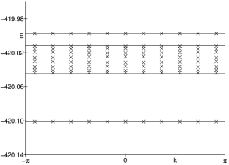
Figure 3: Detail of the eigenvalue spectrum for the generalized QDNLS periodic lattice (2), $n=6$, $f=11$, $\gamma_{1}=30,\gamma_{2}=0,\epsilon=0.5$.

In this case we have a “continuum band” which shows very weak $k$-dependence, plus two “line bands”, one above and one below. With other choices of $\gamma_{1}$ and $\gamma_{2}$ we can move one or both of the “line bands” into the continuum.

Fig 4 shows the corresponding $\{3,3\}$ case.

Figure 4: Detail of the eigenvalue spectrum for (2), $n=6$, $f=11$, $\gamma_{1}=10$, $\gamma_{2}=20$, $\epsilon=0.5$.

In this case there appears to be only two “line bands”, but a closer examination reveals the upper “line” is in fact a continuum band with the degeneracy split at an $O(\epsilon/\gamma)^{3}$ level.

IV.1 Perturbation theory, $n=6$, $\{4,2\}$ band

Proceeding as in the $\{2,2\}$ case, we now obtain

$$H^{(42)}=D\epsilon^{2}\,I_{2\sigma}-\frac{\epsilon^{2}}{\gamma_{1}}\left(\begin{array}[]{ccccc}\Gamma&1&&&p\\ 1&0&1&&\\ &\ddots&\ddots&\ddots&\\ &&1&0&1\\ p^{*}&&&1&\Gamma\\ \end{array}\right)$$ (11)

where

$$D =-\frac{2}{3}\frac{5\gamma_{1}-9\gamma_{2}}{\gamma_{1}(\gamma_{1}-3\gamma_{2})}\ ;\ \Gamma=\frac{2}{3}\frac{4\gamma_{1}^{2}-27\gamma_{2}^{2}}{(\gamma_{1}-3\gamma_{2})(\gamma_{1}-6\gamma_{2})};$$

$$p =\frac{6\gamma_{1}e^{ik}}{\gamma_{1}-6\gamma_{2}}\,.$$

An analysis of the eigenvalues of this matrix in the $f\rightarrow\infty$ limit is somewhat messy but explicit results can be found: details will be published elsewhere. Essentially the results depend on whether two rational functions of $\gamma_{1}/\gamma_{2}$ are less than or greater than 1 in modulus. This gives the two “line bands” in Fig 3. The corresponding eigenstates are essentially symmetric and antisymmetric combinations of the Bloch waves made from $|42\rangle$ and $|24\rangle$.

The “continuum band” is given by the formula

$${E}_{c}=24\gamma_{2}-14\gamma_{1}+\frac{2\epsilon^{2}}{\gamma_{1}}\left[\frac{5\gamma_{1}-9\gamma_{2}}{9\gamma_{2}-3\gamma_{1}}-\cos\theta\right]+{\cal O}\left({\epsilon}^{3}\right),$$ (12)

where $\theta\in(0,\pi)$. Note that, up to order 2 in $\epsilon$, the energies of this band do not depend on the crystal momentum $k$, in accord with the numerical results.

IV.2 Perturbation theory, $n=6$, $\{3,3\}$ band

In this case the correction to the zeroth order states is given by

$$H^{(33)}=\frac{6\epsilon^{2}}{3\gamma_{2}-2\gamma_{1}}\left(\,I_{\sigma}+M\right)$$ (13)

where $M_{1,1}=\Gamma=\frac{9}{2}(2\gamma_{2}-\gamma_{1})/(\gamma_{1}-6\gamma_{2})$ and $M_{i,j}=0$ otherwise. The diagonal matrix (13) has an “impurity” $\Gamma$ responsible for a splitting of the states $|33\rangle$ from the rest of the band. In this respect, the $|33\rangle$’s can be seen as “bound states of doublets” within the $\{3,3\}$-band. Note again that none of the elements of the matrix above contains the wave vector $k$. At this order of perturbation theory, the bands are then flat. Moreover, the degeneracy of the $|3\cdots 3\rangle$’s (i.e. two 3-quanta breathers separated by one or more empty sites) has still not been lifted although it would to next order.

V Discussion

It is possible to generalize the above results to discuss $\{m,\ell\}$ bands when $m+\ell=n>6$. The case $m=\ell$ is similar to the $\{3,3\}$ case and the case $m>\ell>1$ follows the $\{4,2\}$ case discussed above. Details will be given elsewhere.

The results known previously for bound states representing a group of $n$ bosons located on the same site Scott et al. (1994) have been extended here to higher order states representing two interacting groups of bosons. This opens up the possibity of a study of the collision process between these composite particles, that is a quantum breather collision. A similar study has already been done for the continuous version of (1), i.e. the integrable quantum nonlinear Schrödinger equation (QNSE), well known in nonlinear optics Lai89 and quantum field theory Thacker81 . However, the bound states of groups of quanta which we have described here within the $\{m,\ell\}$ bands do not exist in QNSE. Their appearence in these nonintegrable discrete systems is thus expected to affect the collision process between two quantum breathers and to bring new features in comparison to the quantum soliton collisions described in Lai89 . Results of this investigation will be reported elsewhere.