The Propagation of Quantum Information Through a Spin System

Abstract

It has been recently suggested that the dynamics of a quantum spin system may provide a natural mechanism for transporting quantum information. We show that one dimensional rings of qubits with fixed (time-independent) interactions, constant around the ring, allow high fidelity communication of quantum states. We show that the problem of maximising the fidelity of the quantum communication is related to a classical problem in fourier wave analysis. By making use of this observation we find that if both communicating parties have access to limited numbers of qubits in the ring (a fraction that vanishes in the limit of large rings) it is possible to make the communication arbitrarily good.

In quantum information science it is a crucial problem to develop techniques for communicating qubits. A key task is to develop protocols for taking a qubit’s state at one location to another while minimising the degradation of the quantum coherence.

In this paper we consider whether it is possible to use a one dimensional arrangement of qubits – a ring – coupled by nearest-neighbour interactions, to communicate a qubit from one part of the ring to another with high-fidelity.

It is clear that this communication can be done, for example, if one can perform fast local unitary operations on the individual qubits (by fast we mean that the local unitary operations are effectively instantaneous compared with the time it takes the interaction between qubits to change the state appreciably). This is because any nearest-neighbour interaction can be used to perform a swap operation on pairs of qubits Dür et al. (2001); Bennett et al. (2002); Dodd et al. (2002); Khaneja and Glaser (2002). Thus the communication can be performed by putting a given qubit into the state to be communicated and then moving it along the chain of qubits by swapping the state along the line to the required position.

In this paper, however, we have in mind the situation that we do not have access to the whole set of spins during the communication; rather the set of spins behaves more like a fibre into which one can input a qubit state, and hope that the state appears at the other end of the fibre. The question is whether it is possible for a set of spins with only its passive interaction to act as an effective communication channel.

We would also like the qubit fibre to have the property that we could increase the length of the fibre without needing to completely re-fabricate it; thus if we wanted to communicate twice as far we would like to be able to simply add two identical fibres together and find that the fidelity and time of transmission depended in a simple way on the fidelity and time of the individual fibre.

Some interesting work has already been done in this area concerning communication of qubits along a 1D Heisenberg spin chain Bose (2003) (and, more recently, in the $1$D $XY$ model, Subrahmanyam (2003)). In Bose (2003) the aim was to put one qubit in a chain or ring into a given state and to transfer the state, as well as possible, along the chain (or ring) to the output qubit. The input and output qubits were placed at diametrically opposite places in the chain (or ring) and the interaction between neighbouring qubits was time-independent and constant around the length of the system. Interestingly if a ring has length four, there is a time after which the state of the output qubit is precisely the same as that of the input qubit. As the length of the system is increased, however, the maximum fidelity achievable was found to go down with increasing separation. For example, chains of length approximately $80$ have fidelity not much better that $2/3$ (this is the fidelity of the best classical transmission of an unknown qubit); thus the approach would not be useful for transmission over long distances. A further notable feature of the protocol is that the time at which the maximum fidelity is reached does not depend in any simple way on the length of the ring. This is because the maximum fidelity arises when an expression of the form $\sum_{j}e^{i\pi\alpha_{j}t}$ reaches its maximum (where $t$ is the time, and the $\alpha_{j}$ are rational constants which depend on the length of the ring). Thus in this framework there is no natural notion of the speed of transmission along the fibre.

Further progress was made in Christandl et al. (2003) where the authors show that a single qubit can be communicated perfectly in a hypercube geometry. The authors also show how to communicate a qubit perfectly in a linear chain with variable couplings given by a specific arithmetic sequence. Using this idea for communicating arbitrary distances, would however require re-fabricating the channel for each distance.

A further interesting proposal for communicating quantum information using the ground state of a certain spin system has been recently developed in Verstraete et al. (2003). There it was found that perfect transmission is possible when the freedom to apply local measurements on all the spins is allowed.

We can summarise our desiderata in this paper by saying that we wish to develop schemes for high fidelity quantum communication with three essential criteria; (i) Minimum control requirements. We require that it is unnecessary to apply many fast control operations throughout the transmission; (ii) Robustness. We want the device to be capable of tolerating small errors without diminishing the quality of the communication too much; and (iii) Flexibility. We want to be able to change parameters (such as the locations of the communicating parties) simply without requiring a new device be fabricated.

Our proposal makes quantum spin chains behave as a medium through which quantum information propagates. Using the fact that dynamics in restricted subspaces for $1$D quantum spin chains can be described by classical fourier wave analysis we show that there are natural notions of group velocity and dispersion for quantum information. We propose a figure of merit for the information propagation, the qubit rate, and analyse this quantity for a family of ideal and realistic physical models: nearest-neighbour $1$D spin chains. In addition, we argue that our protocols satisfy the requirements (i)-(iii) we outlined in the previous paragraph.

We show how to increase the quality of quantum communication in a variety of realistic spin models by relaxing the restriction that the two parties can only access a single qubit. We allow both parties the ability to access a limited number of extra sites, a fraction which tends to zero as the length of the chain increases. The connection between propagation of quantum information in spin rings and classical fourier wave analysis provides a way to visualise the propagation of quantum information as a pulse through a medium.

We now turn to a precise description of the protocol we will study. We consider a ring of $N$ spin-$1/2$ systems evolving according to a nearest-neighbour hamiltonian $H$. We identify the $(N+1)$th site with the $1$st site, i.e. $A_{N+1}\equiv A_{1}$. We imagine that two parties, Alice $A$ and Bob $B$ are located at sites $1$ and $N/2$, respectively. (We assume, for simplicity, that the ring is composed of an even number of spins. Note, however, that our subsequent results do not depend on this fact.) We suppose that Alice and Bob are able to access a total of $\Lambda$ sites each, centred on the $1$st and $N/2$th sites, respectively. Alice and Bob are allowed to perform any operation allowed by the rules of quantum mechanics on their sites. Finally, we assume that the completely polarised state $|00\cdots 0\rangle$ is an eigenstate of the hamiltonian $H$, and that before the protocol begins the system is prepared in this state.

Alice wants to communicate a (possibly unknown) qubit state $|\psi\rangle$ to Bob. Given a specification of $H$ (assumed to be known to both Alice and Bob) Alice performs some encoding operation $U_{A}$ on her $\Lambda$ qubits. The system is now in the state $|\Psi(0)\rangle=U_{A}|00\cdots 0\rangle$. As the ring is always evolving according to $H$ this state immediately begins to evolve: $|\Psi(t)\rangle=e^{-iHt}|\Psi(0)\rangle$. Bob now waits a certain period of time $T$ which depends only on $H$, $\Lambda$ and $N$, and when this duration elapses he performs a decoding operation $U_{B}$ on his addressable qubits in order to decode or refocus the communicated state into one of the qubits in the ring. (Additionally, Bob could apply a swap operation to move the decoded state into a static register qubit. We prefer to ignore such register qubits because we imagine that decoding unitary operations could also be performed as intermediate steps in a kind of quantum repeater.) The protocol is deemed to succeed when the average fidelity

$$\mathcal{F}(H,N,\Lambda,T,U_{A},U_{B})\triangleq\frac{1}{4\pi}\int d\Omega\,\langle\psi|\rho|\psi\rangle,$$ (1)

where $|\psi\rangle$ is the input state, which we average over the Bloch sphere, and $\rho$ is the decoded output state, is above some prespecified threshold value $\tau$.

Ultimately we are interested in how well a spin ring performs as a conduit for quantum information. In this more general scenario we allow Alice and Bob the freedom to apply a number of encoding/decoding operations in succession. The objective is to maximise the number of qubits successfully communicated (i.e. when $\mathcal{F}\geq\tau$) per unit time. Write the maximum number of qubits that can successfully communicated (where the maximum is taken over the encoding/decoding operations) in a duration $T$ as $M_{\tau}(T)$. We define the long-time average $Q_{\tau}(H)\triangleq\lim_{T\rightarrow\infty}\frac{1}{T}M_{\tau}(T)$ to be the qubit rate for $H$.

Obviously the evaluation of $Q_{\tau}(H)$ is extremely difficult, even for the simplest systems. We only obtain lower bounds for this quantity for a class of rotationally invariant nearest-neighbour hamiltonians.

There is a simple case where we can evaluate $Q_{\tau}(H)$ exactly, namely when $H$ is a hamiltonian corresponding to the translation operator $H=-i\log(\mathcal{T})$, where $\mathcal{T}$ is defined by the following action on computational basis vectors, $\mathcal{T}(|a_{1},a_{2},\ldots,a_{N}\rangle)\triangleq|a_{2},a_{3},\ldots,a_{N},a_{1}\rangle$. When $H$ is of this form the qubit rate takes the maximum value $Q_{\tau}(H)=1$ for all $\tau$. (We have adopted rescaled time units; we will discuss how to calculate the constant of rescaling later.) In order to see this first note that when $t=n$ is an integer the propagator $U(n)=e^{-iHn}=\mathcal{T}^{n}$ is a power of the translation operator. To achieve the qubit rate, Alice needs to encode the state of a qubit into one site of the ring at every integral $t$.

As we’ll argue presently, every hamiltonian $H$ corresponding to the translation operation is massively nonlocal and contains interaction terms between many separated subsystems. For this reason it is unlikely that a system will be fabricated which naturally evolves according to $H$.

Consider now the translation operator $\mathcal{T}$. It is easy to see that the action of $\mathcal{T}$ on computational basis states breaks up into blocks, for example, the states $|00\cdots 0\rangle$ and $|11\cdots 1\rangle$ form blocks all by themselves, and the states $|j\rangle$, $j=1,\ldots,N$, where $|j\rangle$ denotes the state of all $|0\rangle$’s with a $|1\rangle$ in the $j$th site, form a block (we’ll often refer to these states as one-particle states). The remaining basis states each segregate into blocks in a similar fashion. Consider a block of states of size $M$. Choose a state from this block and call it $|\alpha_{1}\rangle$. Every state $|\alpha_{k}\rangle$ within the block can be written as $|\alpha_{k}\rangle=\mathcal{T}^{k-1}|\alpha_{0}\rangle$. Using these $M$ states one can construct $M$ eigenstates of $\mathcal{T}$: $|\beta_{k}\rangle=1/\sqrt{M}\sum_{j=1}^{M}\nu^{(j-1)k}|\alpha_{j}\rangle$, where $\nu=e^{\frac{2\pi}{M}i}$ is the $M$th root of unity. We note that each set of eigenstates so constructed is a quantum fourier transform of the set $\{|\alpha_{j}\rangle\,|\,j=1,\ldots,M\}$. Performing this procedure for each block gives rise to the complete set of eigenstates for $\mathcal{T}$.

We study the qubit rate for the class of rotationally invariant nearest-neighbour spin-$1/2$ models. Because of the rotational invariance $[H,\mathcal{T}]=0$ and we may simultaneously diagonalise both $H$ and $\mathcal{T}$. We restrict our attention further to the class of $1$D spin rings which fix the following special eigenstates of $\mathcal{T}$, which we call the twisted $W$-states, $|W(k)\rangle\triangleq\frac{1}{\sqrt{N}}\sum_{j=1}^{N}\mu^{(j-1)k}|j\rangle$, where $\mu$ is the $N$th root of unity $\mu=e^{\frac{2\pi}{N}i}$. All the protocols we describe in this paper take place in the subspace formed by the twisted $W$-states.

The spin hamiltonian $H$ fixes the states $|W(k)\rangle$ with eigenvalues $\omega(k)$ (and also, via a rescaling of energy, $H$ fixes $|00\cdots 0\rangle$ with eigenvalue $0$). Suppose we start the system in the arbitrary state $|\Psi(0)\rangle=\alpha|00\cdots 0\rangle+\beta\sum_{j=1}^{N}c_{j}|j\rangle$, where $|\alpha|^{2}+|\beta|^{2}=1$ and $\sum_{j=1}^{N}|c_{j}|^{2}=1$. The subsequent time evolution of this state can be written

$$|\Psi(t)\rangle=\alpha|00\cdots 0\rangle+\beta\sum_{k=1}^{N}\tilde{c}_{k}e^{-i\omega(k)t}|W(k)\rangle,$$ (2)

where $\tilde{c}_{k}=\frac{1}{\sqrt{N}}\sum_{j=1}^{N}{\mu^{-(j-1)k}c_{j}}$. The coefficient $c_{j}(t)$ of the $|j\rangle$ term can be found as

$$c_{j}(t)=\frac{1}{\sqrt{N}}\sum_{k=1}^{N}\tilde{c}_{k}e^{-i\omega(k)t+2\pi i(j-1)k/N}.$$

Because the dynamics only take place in the zero- and one-particle subspace we can establish the following useful result. Suppose $\alpha=0$. If we bipartition the spin system into two subsystems $A$ and $\overline{A}$ we can always write the system’s state $|\Psi(t)\rangle=\sum_{j=1}^{N}e_{j}(t)|j\rangle$ in the following way,

$$|\Psi(t)\rangle=\sqrt{1-\mathcal{C}_{\overline{A}}(t)}|\phi\rangle_{A}|\mathbf{0}\rangle_{\overline{A}}+\sqrt{\mathcal{C}_{\overline{A}}(t)}|\mathbf{0}\rangle_{A}|\phi^{\prime}\rangle_{\overline{A}},$$ (3)

where

$$\mathcal{C}_{\overline{A}}(t)=\sum_{j\in\overline{A}}|e_{j}(t)|^{2},$$

$$|\phi\rangle=\frac{1}{\sqrt{1-\mathcal{C}_{\overline{A}}(t)}}\sum_{j\in A}e_{j}(t)|j\rangle,$$

and

$$|\phi^{\prime}\rangle=\frac{1}{\sqrt{\mathcal{C}_{\overline{A}}(t)}}\sum_{j\in\overline{A}}e_{j}(t)|j\rangle.$$

Note that Eq. (3) is a two-term Schmidt decomposition of $|\Psi(t)\rangle$ because ${}_{A}\langle\phi|\mathbf{0}\rangle_{A}={}_{\overline{A}}\langle\phi^{\prime}|\mathbf{0}\rangle_{\overline{A}}=0$.

When Alice wants to send the state $|\psi\rangle=\alpha|0\rangle+\beta|1\rangle$ she will encode this state as $\alpha|00\cdots 0\rangle+\beta\sum_{j=1}^{N}c_{j}(0)|j\rangle$, where she is free to choose nonzero $c_{j}(0)$ as long as the index $j$ lies within her subset of addressable spins. After time $T$ has elapsed then this state can be written, following the discussion in the previous paragraph, as

$$|\Psi(T)\rangle=\beta\sqrt{1-\mathcal{C}_{B}(T)}|\eta\rangle_{\overline{B}}|\mathbf{0}\rangle_{B}+\\ |\mathbf{0}\rangle_{\overline{B}}(\alpha|\mathbf{0}\rangle_{B}+\beta\sqrt{\mathcal{C}_{B}(T)}|\eta^{\prime}\rangle_{B}),$$ (4)

where now the bipartition is given by $\overline{B}B$, where $B$ is Bob’s addressable spins and $\overline{B}$ now refers to all the other spins and

$$\mathcal{C}_{B}(T)=\sum_{j\in B}|e_{j}(t)|^{2}.$$

Bob now applies a decoding unitary $U_{B}$ to his part $B$ of the ring. The unitary is (partially) defined by $U_{B}|\mathbf{0}\rangle_{B}=|\mathbf{0}_{B}\rangle$ and $U_{B}|\eta^{\prime}\rangle_{B}=|{N/2}\rangle$. (There is a great deal of arbitrariness in how Bob decodes his state. We choose to concentrate the state into one qubit in order to facilitate the evaluation of the average fidelity of the channel.)

After decoding, the state $\rho$ of the qubit $N/2$ has density operator

$$\rho=\left(\begin{matrix}|\alpha|^{2}+|\beta|^{2}(1-\mathcal{C}_{B}(T))&\sqrt{\mathcal{C}_{B}(T)}\alpha\beta^{*}\\ \sqrt{\mathcal{C}_{B}(T)}\alpha^{*}\beta&|\beta|^{2}\mathcal{C}_{B}(T)\end{matrix}\right)$$ (5)

with respect to the basis $\{|0\rangle_{N/2},|1\rangle_{N/2}\}$ of qubit $N/2$. This state may be written $\rho=\mathcal{E}_{T}(|\psi\rangle_{N/2}\langle\psi|)=M_{0}|\psi\rangle_{N/2}\langle\psi|M_{0}^{\dagger}+M_{1}|\psi\rangle_{N/2}\langle\psi|M_{1}^{\dagger}$, where $|\psi\rangle_{N/2}=\alpha|0\rangle_{N/2}+\beta|1\rangle_{N/2}$ and $M_{0}$ and $M_{1}$ are the Kraus operators of an amplitude damping channel $\mathcal{E}$,

$$M_{0}=\left(\begin{matrix}1&0\\ 0&\sqrt{\mathcal{C}_{B}(T)}\end{matrix}\right)$$

and

$$M_{1}=\left(\begin{matrix}0&\sqrt{1-\mathcal{C}_{B}(T)}\\ 0&0\end{matrix}\right),$$

with respect to the basis $\{|0\rangle_{N/2},|1\rangle_{N/2}\}$ (cf. Bose (2003)).

The fidelity $\langle\psi|U_{B}\rho U_{B}^{\dagger}|\psi\rangle$ of Bob’s state with the input state is given by

$$|\alpha|^{4}+(1+2\sqrt{\mathcal{C}_{B}(T)}-\mathcal{C}_{B}(T))|\alpha|^{2}|\beta|^{2}+\mathcal{C}_{B}(T)|\beta|^{4}.$$ (6)

The average fidelity Eq. (1) can be evaluated as $\frac{1}{2}+\frac{1}{3}\sqrt{\mathcal{C}_{B}(T)}+\frac{1}{6}\mathcal{C}_{B}(T)$. This function depends monotonically on the quantity $\mathcal{C}_{B}(T)$.

It is clear from the discussion in the preceding paragraphs that the quantity $\mathcal{C}_{B}(T)$ plays a central role in determining the effectiveness of the communication protocol. We now study this quantity further, and show how to reduce the problem of its maximisation to a well-known type of problem in Fourier wave analysis.

Motivated by the importance of $\mathcal{C}_{B}(T)$ we introduce a method for visualising quantum states which lie within the one-particle subspace. Given such a state $|\nu\rangle=\alpha|00\cdots 0\rangle+\beta\sum_{j=1}^{N}c_{j}|j\rangle$, we visualise it by plotting the quantities $\nu_{j}\triangleq|c_{j}|^{2}$ against site number. Clearly the area under the resulting (bar) graph equals $1$. Obviously this pictorial representation does not represent any of the phase information contained in the system’s state. However, this phase information plays no part in the quantity we are interested in, $\mathcal{C}_{B}(T)$, which is simply the area under the graph of the state $|\nu(T)\rangle$ between sites $N/2-\Lambda/2,\ldots,N/2+\Lambda/2$. The graph of the system’s state $|\nu(T)\rangle$ is given by

$$\nu_{j}(T)=\frac{1}{N}\left|\sum_{k=1}^{N}\tilde{c}_{k}e^{-i\omega(k)t+2\pi i(j-1)k/N}\right|^{2}.$$

It is worth emphasising that the method we have just introduced for visualising quantum states of the ring depends crucially on the properties of our spin systems. The dynamics for the ring occurs solely within the zero- and one-particle subspaces spanned by $|\mathbf{0}\rangle$ and $\{|j\rangle\,|\,j=1,\ldots,N\}$. This subspace scales linearly with the ring. It is precisely this feature which facilitates our construction for the graph of the state, which is essentially a method for representing, visually, a linear number (in $N$) of degrees of freedom.

The problem of maximising the area under the graph $\nu_{j}(T)$ between certain sites is a well-known a classical problem in fourier wave analysis; our problem has reduced to studying the linear dynamics of superpositions of complex scalar waves. The quantity $\omega(k)$ is the dispersion relation and the position variable is given by $x_{j}=(j-1)/N$. We wish to work out an assignment $c_{j}(0)$ of initial amplitudes in Alice’s subsystem, or a wavepacket of quantum information, so that subsequent evolution preserves as much of the width and integrity of the wavepacket as possible.

Given a specification of the dispersion relation $\omega(k)$ we have all the information we require to embark on the design of wavepackets which preserve their shape. These numbers are, of course, the eigenvalues of $H$ for the eigenstates $|W(k)\rangle$.

To illustrate our ideas in the following we use the Heisenberg model on $N$ sites

$$H=\chi\frac{N}{2}I-\frac{\chi}{2}\sum_{j=1}^{N}\boldsymbol{\sigma}_{j}\cdot\boldsymbol{\sigma}_{j+1},$$

where we have introduced an arbitrary constant $\chi$. We will explain which value of $\chi$ we choose in the following. The dispersion relation for the Heisenberg model is $\omega(k)=2\chi\left(1-\cos(\frac{2\pi k}{N})\right)$. (We have rescaled the zero of energy for the Heisenberg model so that $|\mathbf{0}\rangle$ has eigenvalue zero.)

Currently our problem is not identical to the well-studied problems in wave motion (see, for example, Whitham (1999)). The difference is that we are dealing with wave motion in a discrete system whereas most of the theory of wave motion (at least in regards to the design of optimal wavepackets) is for continuous systems. In the subsequent discussion we will make use of the results from the continuous theory, but it must be understood that these results only hold asymptotically in the limit where $N\rightarrow\infty$ and the intersite spacing $\delta\rightarrow 0$. In particular, we emphasise that the appearance of derivatives must be understood as a formal device and really only make sense in this limit. We’ll justify the applicability of these asymptotic results presently by comparing them with numerical results.

In classical fourier wave theory the concept of group velocity plays a crucial role in the design of wavepackets which preserve their shape as time evolves Whitham (1999). The group velocity $v(k_{0})$ for a wavenumber $k_{0}$ is defined to be $v(k_{0})=\frac{1}{2\pi}\frac{d\omega(k)}{dk}\big{|}_{k=k_{0}}$. (For the models we consider we are given a specification of $\omega(k)$ which makes sense for fractional $k$, so that it is possible to compute this derivative.) The significance of this quantity is that an initial wavepacket $\sum_{k=1}^{N}w_{k}e^{2\pi ix_{j}k}$ consisting of fundamental waves with large amplitude focussed on wavenumber $k_{0}$ will translate with velocity $v(k_{0})$ as time evolves.

Unless the system is dispersionless ($\omega(k)=ck$) the initial wavepacket will spread as time evolves Whitham (1999). The rate-of-spread of the initial wavepacket is proportional to the second order term $\frac{1}{2\pi}\frac{d^{2}\omega(k)}{dk^{2}}\big{|}_{k=k_{0}}$. If this derivative is zero (as will be the case in one of the models we consider) there is no appreciable spread of the wavepacket to second order in $\omega(k)$. There may, however, be contributions from third and higher order terms, which cause an initial wavepacket to spread.

The generic strategy Jackson (1999) for designing wavepackets which change shape as little as possible is to use a gaussian-modulated wave of variance $\Delta$ centred at position $x_{k}$ and wavenumber $k_{0}$ corresponding to the maximum available group velocity $v(k_{0})$. In our case the “wave” is a twisted $W$-state, so this “wavepacket” is written $|\Psi(0)\rangle=\alpha|\mathbf{0}\rangle+\beta|G(x_{k},k_{0},\Delta)\rangle$, where

$$|G(x_{k},k_{0},\Delta)\rangle=1/\sqrt{\mathcal{N}}\sum_{j=1}^{N}e^{-\frac{(x_{j}-x_{k})^{2}}{2\Delta^{2}}+2\pi ik_{0}x_{j}}|j\rangle$$

and $\mathcal{N}$ is chosen to normalise the state. The graph for the initial state is given by

$$\Psi_{j}(0)=\frac{1}{\mathcal{N}}\left|\sum_{j=1}^{N}e^{-\frac{(x_{j}-x_{i})^{2}}{2\Delta^{2}}+2\pi ik_{0}x_{j}}\right|^{2}.$$

This state has exactly the form of a gaussian-modulated complex scalar wave centred around wavenumber $k_{0}$ and with (spatial) width $L$. (We define width $L$ to be when more than some prespecified area, say 95%, lies within an interval $L$ centred on the maximum of the gaussian. We note that $L$ is some multiple of $\Delta$. Throughout the remainder of this paper we choose $L=4\Delta$.)

It is known that an initial gaussian wavepacket, under time-evolution, remains, to good approximation, a gaussian of width $L(t)$ satisfying Jackson (1999)

$$\frac{L(t)}{L(0)}=\left[1+\left(\frac{\omega^{\prime\prime}(k_{0})t}{L^{2}(0)}\right)^{2}\right]^{\frac{1}{2}}.$$ (7)

Because Alice is assumed able to address only $NL(0)$ sites (recall we have rescaled the length of the ring to be $1$ by defining the position variable $x_{j}=(j-1)/N$) we propose using the gaussian initial pulse introduced in the previous paragraph truncated (and renormalised) after $NL(0)$ sites.

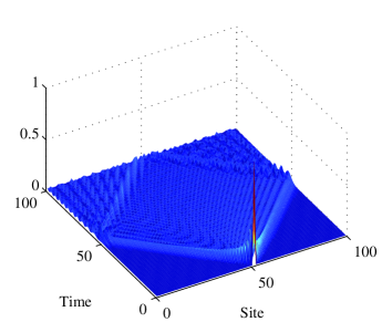
Figure 1: Propagation of the state $|N/2\rangle$ in a $100$-site Heisenberg spin ring.

Figure 2: Propagation of a truncated gaussian-modulated $W$-state of width $10$ and wavenumber $N/4$ in a $100$-site Heisenberg spin ring.

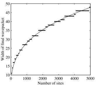
Figure 3: Dots: size of the final wavepacket in the Heisenberg spin ring for $N=50$ to $N=5000$. (Initial wavepacket is a gaussian modulated wave of variance ${N}^{\frac{1}{3}}$ truncated after $2{N}^{\frac{1}{3}}$ sites.) Final width $F$ is defined to be when more than $95\%$ of the wavepacket lies between $F$ sites. Solid line: graph of $2.8{N}^{\frac{1}{3}}$ for comparison. The apparent jumps of integer amounts greater than $1$ in the numerical results is an artifact of the way the width of the final wavepacket is calculated. The final wavepacket has a sequence trailing oscillations. In order to get an area of more than some arbitrary amount (like $0.95$) it is sometimes necessary to include several more sites in a go.

We want to design a wavepacket that spreads by an amount that scales favourably with $N$. We demand that a wavepacket of width $L$ spreads by only a constant factor to a final width of $L^{\prime}\approx\kappa L$ by the time it reaches Bob. To simplify the discussion we note that for typical wavenumbers close to $k_{0}$ we have $\omega^{\prime\prime}(k_{0})=\lambda/N^{2}$ (this is true of all the models we consider). We analyse the scaling, with $t\approx N$ (the time it takes for a wavepacket to traverse the ring), of the spread $S(N)$ of the wavepacket: $S(N)=L(N)/L(0)=\left[1+\left(\frac{\lambda}{NL^{2}(0)}\right)^{2}\right]^{\frac{1}{2}}$. If we want the final width of the wavepacket to be independent of the length of the ring we need to choose $L(0)=1/\sqrt{N}$. This means that the initial packet needs to be supported on a subsystem containing on the order of $\sqrt{N}$ sites. In the “mesoscopic” limit of large but finite $N$ the fraction of the ring that Alice and Bob need to access can be made arbitrarily small (it scales as $N^{-\frac{1}{2}}$).

We now analyse these results for the Heisenberg model. We want a signal pulse to travel as fast as possible. Looking at the group velocity $\omega^{\prime}(k)=\frac{2\chi}{N}\sin(\frac{2\pi}{N}k)$ we find that this occurs for $k=N/4,3N/4$, $\nu(k)=\pm\frac{2\chi}{N}$. At this point we choose $\chi=1/4$. We do this so that the final wavepacket will arrive at Bob’s portion of the ring at time $t=N$ (recall that Alice and Bob are separated by a distance $N/2$). So we choose the initial wavepacket to be a truncated gaussian-modulated superposition of width $\sqrt{N}$ of twisted $W$-states centred around $k=N/4$.

The case of wavepackets centred on $k_{0}=N/4$ is rather special — note that the dispersion $\omega^{\prime\prime}(k_{0})$ for this model is identically $0$. Naïvely applying formula Eq. (7) for the spread of the wavepacket suggests that an initial wavepacket of any width will not spread at all. This is an artifact of our approximation; we assumed that the dispersion relation could be expanded and truncated at second order with little error. In the special situation where $\omega^{\prime\prime}(k_{0})$ vanishes we need to go to third order. For this case a gaussian pulse does not remain a gaussian. (Instead, it becomes an Airy function Agrawal (2002).) The formula Eq. (7) is invalid in this case and we need to use the third-order broadening factor Agrawal (2002)

$$\frac{L(t)}{L(0)}=\left[1+\frac{1}{2}\left(\frac{\omega^{\prime\prime\prime}(k_{0})t}{\sqrt{2}L^{3}(0)}\right)^{2}\right]^{\frac{1}{2}}.$$

We solve this equation for $t=N$ to find the width $L(0)$ of initial wavepacket which has constant spread with $N$. We find that $L(0)$ need only scale as $N^{-\frac{2}{3}}$. Such a wavepacket consists of $NL(0)=N^{\frac{1}{3}}$ sites.

We illustrate these results for the Heisenberg ring of $N=100$ sites in Fig. (1) and Fig. (2). By way of contrast, in Fig. (1) we first show the dynamics of the state with a single $|1\rangle$ at site $N/2$ (this type of localised initial state is what is used in the protocols of Bose (2003), Subrahmanyam (2003) and Christandl et al. (2003)). Because the state $|N/2\rangle$ is an equal superposition of all the twisted $W$-states all the waves are involved in the dynamics and hence the initial packet disperses rapidly. In Fig. (2) we see that the shaped pulse retains its shape for much longer durations. This is because fewer waves are involved in the superposition. We note that, generically, for wavepackets centred around wavenumbers not equal to $N/4$ a square-root scaling for the final wavepacket is observed.

Before we conclude our discussion of the numerical results we refer to Fig. (3). In this graph we have plotted, for the Heisenberg ring, the width of the final wavepacket (we define the width $F$ to be when more than $95\%$ of the area lies within $F/2$ sites either side of site $N/2$) for rings of sizes $50$ through $5000$ sites. We have also plotted $2.8{N}^{\frac{1}{3}}$ for comparison. Because the Heisenberg model is diffusionless to second order in the dispersion relation $\omega^{\prime\prime}(k_{0})=0$, we expect that the numerically recorded spread ought to be smaller than the spread predicted for models with second-order dispersion. We can see, from Fig. (3) that this is indeed the case. For $N=5000$ the proportion of the ring that Alice and Bob must be able to access is less than $1\%$ each.

To conclude we construct all the rotationally invariant nearest-neighbour spin hamiltonians which fix the $|\mathbf{0}\rangle$ and twisted $W$-states. An easy way to construct all such hamiltonians is to first assume that the hamiltonian preserves $S^{z}\triangleq\sum_{j=1}^{N}\sigma_{j}^{z}$. Any such hamiltonian may be written as

$$H=c_{0}I+\sum_{j=1}^{N}\Big{[}c_{1}\sigma^{+}_{j}\sigma^{-}_{j}+c_{2}\sigma^{-}_{j}\sigma^{+}_{j}+d_{1}(\sigma^{+}_{j}\sigma^{-}_{j+1}+\sigma^{-}_{j}\sigma^{+}_{j+1})\\ +d_{2}(\sigma^{+}_{j}\sigma^{-}_{j+1}+\sigma^{-}_{j}\sigma^{+}_{j+1})^{2}+e_{1}i(\sigma^{+}_{j}\sigma^{-}_{j+1}-\sigma^{-}_{j}\sigma^{+}_{j+1})\\ +f_{1}i(\sigma^{+}_{j}\sigma^{-}_{j+1}-\sigma^{-}_{j}\sigma^{+}_{j+1})(\sigma^{+}_{j}\sigma^{-}_{j+1}+\sigma^{-}_{j}\sigma^{+}_{j+1})\Big{]},$$ (8)

where $\sigma^{\pm}_{j}\triangleq\frac{1}{2}(\sigma^{x}_{j}\pm i\sigma^{y}_{j})$. It may be verified, with a little algebra, that this is the most general rotationally invariant nearest-neighbour hamiltonian which nontrivially fixes the twisted $W$-states. (There is one additional term which fixes the twisted $W$-states, $\sigma^{-}_{j}\sigma^{-}_{j+1}$, however, it trivially annihilates these states and thus contributes nothing to the dispersion relation. Note also that the $f_{1}$ term annihilates the twisted $W$-states.)

The hamiltonian Eq. (8) gives rise to the following dispersion relation

$$\omega(k)=A+B\cos\left(\frac{2\pi}{N}k\right)+B^{\prime}\sin\left(\frac{2\pi}{N}k\right),$$ (9)

where $A=c_{0}+c_{1}(N-1)+c_{2}+2d_{2}$, $B=2d_{1}$ and $B^{\prime}=-2e_{1}$. We note that both the Heisenberg model in a magnetic field and the $XY$ model in a magnetic field can both be expressed as in Eq. (8) for specific choices of $c_{j}$, $d_{j}$, $e_{1}$ and $f_{1}$. The dispersion relation Eq. (9) is no more general than that for the Heisenberg model so all of our discussion concerning the design of optimal signals for the Heisenberg model carries through straightforwardly for the general class of models Eq. (8).

We see from the dispersion relation Eq. (9) that the most general rotationally invariant nearest-neighbour hamiltonian fixing the twisted $W$-states is dispersive. This shows us that, in order for a hamiltonian $H$ to exponentiate to the translation operator $\mathcal{T}=e^{iH}$, it is necessary for $H$ to contain interaction terms between separated parties. This verifies our earlier claim that such a hamiltonian must be nonlocal.

Finally, we note that our results imply that the qubit rate for a rotationally invariant nearest-neighbour Hamiltonian on $N$ sites is bounded below: $Q_{0.95}(H)\geq 1/N$.

We have introduced a method for improving the quantum communication characteristics of $1$D quantum spin rings. According to the connection between the dynamics of quantum information in these rings with fourier wave analysis we have been able to import many of the results concerning the design of signals which disperse minimally. Clearly our results illustrate that our communication protocol has minimal control requirements and is flexible. We have not tackled the problem of determining the resistance of our protocol to error.

Many future problems suggest themselves at this stage. Perhaps the most interesting is the extension of the results to linear chains. In this case our results cannot be applied because the twisted $W$-states are not eigenstates for nearest-neighbour hamiltonians on a chain. However, a generalisation of our method of pulse shaping ought to be possible. Another important future problem concerns the resistance of the protocol to errors. We believe that the protocol is robust, but a full analysis needs to be done. Finally, we note that all our protocols take place in the single-particle subspace. The dimension of this subspace increases linearly with increasing numbers of qubits; however the hilbert space of the system increases exponentially with $N$. Perhaps it is possible to increase the qubit rate substantially by taking advantage of larger subspaces which include two and higher particles. Further investigations along these lines are being conducted.