Dynamics of a large spin with weak dissipation

Abstract

We investigate the generalization of the spin-boson model to arbitrary spin size. The Born-Markov approximation is employed to derive a master equation in the regime of small coupling strengths to the environment. For spin one half, the master equation transforms into a set of Bloch equations, the solution of which is in good agreement with results of the spin-boson model for weak ohmic dissipation. For larger spins, we find a superradiance-like behavior known from the Dicke model. The influence of the nonresonant bosons of the dissipative environment can lead to the formation of a beat pattern in the dynamics of the $z$-component of the spin. The beat frequency is approximately proportional to the cutoff $\omega_{c}$ of the spectral function.

, , and

1 Introduction

The influence of a dissipative environment on the behavior of a two-state system is often studied within the spin-boson model [1]. This model applies to many systems from various fields of physics such as a magnetic flux in a SQUID, electrons tunneling in chemical systems or double quantum dots, and two-level systems in glasses [2]. Naturally, there are other systems which are described by a spin greater than one half. Nuclear spins constitute one example. The elements gallium and arsenic used in the majority of modern solid state experiments have a nuclear spin of 3/2. The nuclear relaxation process measured in NMR experiments [3] is determined by the interaction with a dissipative environment, for instance a two-dimensional electron gas [4]. Recent experiments have also been performed on molecular magnets. These are small clusters of a few atoms embedded into a crystal, which can be described as large spins, the most prominent examples of which (Mn₁₂ and Fe₈) are believed to have a total spin of 10 [5, 6].

Large spins also describe dissipation-induced collective effects of an ensemble of identical two-level systems. The coupling to the common dissipative environment introduces an indirect interaction between the otherwise independent systems. A pseudo-spin – formally the sum of all spin one halfs – gives information about the degree of polarization of the ensemble.

In this work, we employ a master equation for the description of the large spin derived within the Born-Markov approximation. The validity of the latter seems to be sometimes controversial in the literature, and our aim is to demonstrate that a careful derivation in the exact eigenstate basis of the coherent system indeed yields reliable results down to zero temperature for all parameter values, as long as the dissipative coupling (parameter $\alpha$) is small.

2 Model Hamiltonian

We take the examples of section 1 as a motivation to study the generalization of the spin-boson model to larger spins, referred to as the large-spin model in the following. The Hamiltonian is given by

$$H=\varepsilon\,J_{z}+2T_{c}\,J_{x}+J_{z}\sum_{q}\gamma_{q}\,(a_{q}^{\dagger}+a_{-q})+\sum_{q}\omega_{q}\,a_{q}^{\dagger}a_{q}.$$ (1)

The $J_{i}$ are components of a spin vector $\bm{J}$ of arbitrary size $J$. For $J\!=\!1/2$, the model reduces to the spin-boson system. The bias is given by $\varepsilon$ and $T_{c}$ accounts for tunneling between adjacent eigenstates of $J_{z}$. The dissipative environment is modeled by a bath of harmonic oscillators with creation operators $a_{q}^{\dagger}$ for a boson in mode $q$ and interaction strength $\gamma_{q}$ to the spin. The collective character of the model is due to the spin algebra which leads to non-constant tunnel rates for transitions between the different states of the system.

The generalization of the spin-boson model to a dissipative multistate system has been studied by several authors [7, 8, 9, 1]. There, a particle tunnels between different sites with a constant tunnel rate, equivalent to a tight-binding model. Another possible generalization of the spin-boson model arises if also excited states in a double-well potential are considered [10, 11]. All these systems do not show any collective behavior by definition.

The Hamiltonian (1) also differs from the above cited generalizations of the spin-boson model with respect to the interaction term. No counter term in the form of $J_{z}^{2}$ is included in equation (1). Such a term does not occur if e. g. collective effects of an ensemble of two-level systems are described by the large spin. However, it is interesting to note in this context that a quadratic term, $J_{z}^{2}$, can appear in the opposite limit, the strong-coupling regime, of the large-spin model. This is the case if a polaron transformation is applied to the Hamiltonian (1). That term has considerable consequences on the dynamics of the large spin [12].

The Hamiltonian of a large spin with dissipation is closely related to the Dicke-model, described by the Hamiltonian

$$H_{\rm Dicke}=\omega_{\rm D}\,J_{z}+J_{x}\sum_{q}\gamma_{q}\,(a_{q}^{\dagger}+a_{-q})+\sum_{q}\omega_{q}\,a_{q}^{\dagger}a_{q}.$$ (2)

The Dicke Hamiltonian is frequently applied in the field of quantum optics, where it describes an ensemble of independent two-state atoms interacting via the common radiation field. This model exhibits the effect of superradiance as pointed out by Dicke in the original work in 1954, Ref. [13]. The decay of an ensemble of initially excited atoms is not exponential anymore, as one would expect from independent atoms. Instead, the time of the decay decreases inversely with the number of atoms and the maximum intensity of the emitted radiation increases with the square of the number of atoms. The Dicke model does not include direct, electrostatic tunnel coupling terms. The coupling to the environment is offdiagonal in contrast to the spin-boson model where the coupling is diagonal, i.e. to the $z$-component of the spin. For zero bias, $\varepsilon\!=\!0$, the large-spin Hamiltonian reduces to the Dicke model, though in a rotated frame of reference. Thus, the $x$-component of the large-spin model shows superradiant behavior in an unbiased system. We will find that a similar statement applies for the $z$-component of the large spin in a biased system.

3 Master Equation in Born-Markov Approximation

We consider the regime of weak interactions between the large spin and the dissipative environment. The Born-Markov approximation is employed to derive a master equation for the density matrix of the spin. This method is perturbative in the system-reservoir coupling. In second order, the master equation for the density matrix $\rho(t)$ of the spin reads [14]

$$\dot{\tilde{\rho}}(t)=-\int_{0}^{t}\!dt^{\prime}\;{\rm Tr}_{\rm Res}\Big{\{}\big{[}\tilde{V}(t),\big{[}\tilde{V}(t^{\prime}),\tilde{\rho}(t)\otimes R_{0}\big{]}\big{]}\Big{\}}.$$ (3)

The interaction part of the Hamiltonian, Eq. (1), is denoted by $V$, the equilibrium density matrix of the environment by $R_{0}$, and the tilde indicates the interaction picture. The advantage of a master equation in this form is that only operators refering to the spin system enter. The degrees of freedom of the reservoir are already traced out with the understanding that backaction effects on the bosonic bath can be neglected.

In (3), it is assumed that the spin is brought into contact with the environment at time $t\!=\!0$. Hence, the initial density matrix of the system factorizes in a spin and a reservoir part. For finite times, $t\!>\!0$, correlations between the subsystems evolve. These correlations are neglected on the right hand side of equation (3) in the second order Born approximation as they lead to effects of third or higher order in the coupling. Moreover, the Markov approximation assumes that the kernel of the integration in Eq. (3) given by terms like ${\rm Tr}_{\rm Res}\{\tilde{V}(t)\tilde{V}(t^{\prime})R_{0}\}$ decays on a timescale much shorter than the typical timescale of the spin density matrix $\tilde{\rho}(t)$. This is reasonable for weakly interacting systems since the dynamics of the spin in the interaction picture is solely caused by the coupling to the environment. Non-Markovian effects in the Born approximation for $J=1/2$ have been discussed recently by Loss and DiVincenzo [15].

Inserting $\tilde{V}(t)$ in the master equation (3) and transforming back into Schrödinger picture yields the final form of the master equation for a large spin,

$$\begin{split}\dot{\rho}(t)=\;&i\,\big{[}\rho(t),\varepsilon J_{z}+2T_{c}\,J_{x}\big{]}-\frac{1}{\Delta^{2}}\,(\varepsilon^{2}\,\Gamma+4T_{c}^{2}\,\Gamma_{c})\,\big{[}J_{z},J_{z}\,\rho(t)\big{]}\\[2.84526pt] &-\frac{2T_{c}\,\varepsilon}{\Delta^{2}}\,(\Gamma-\Gamma_{c})\,\big{[}J_{z},J_{x}\,\rho(t)\big{]}+\frac{2T_{c}}{\Delta}\,\Gamma_{s}\,\big{[}J_{z},J_{y}\,\rho(t)\big{]}\\[2.84526pt] &+\frac{1}{\Delta^{2}}\,(\varepsilon^{2}\,\Gamma^{*}+4T_{c}^{2}\,\Gamma_{c}^{*})\,\big{[}J_{z},\rho(t)\,J_{z}\big{]}\\[2.84526pt] &+\frac{2T_{c}\,\varepsilon}{\Delta^{2}}\,(\Gamma^{*}-\Gamma_{c}^{*})\,\big{[}J_{z},\rho(t)\,J_{x}\big{]}-\frac{2T_{c}}{\Delta}\,\Gamma_{s}^{*}\,\big{[}J_{z},\rho(t)\,J_{y}\big{]}.\end{split}$$ (4)

Here, the influence of the environment is expressed by the rates

$$\begin{split}\Gamma_{c}&=\frac{\pi}{2}\;\rho(\Delta)\,\coth\!\Big{(}\frac{\beta\Delta}{2}\Big{)}-\frac{i}{2}\;\mathchoice{{\vbox{\hbox{$\textstyle-$}}\kern-4.86108pt}}{{\vbox{\hbox{$\scriptstyle-$}}\kern-3.25pt}}{{\vbox{\hbox{$\scriptscriptstyle-$}}\kern-2.29166pt}}{{\vbox{\hbox{$\scriptscriptstyle-$}}\kern-1.875pt}}\!\int_{0}^{\infty}\!d\omega\;\rho(\omega)\;\Big{(}\frac{1}{\omega+\Delta}+\frac{1}{\omega-\Delta}\Big{)},\\[5.69054pt] \Gamma_{s}&=\frac{1}{2}\;\mathchoice{{\vbox{\hbox{$\textstyle-$}}\kern-4.86108pt}}{{\vbox{\hbox{$\scriptstyle-$}}\kern-3.25pt}}{{\vbox{\hbox{$\scriptscriptstyle-$}}\kern-2.29166pt}}{{\vbox{\hbox{$\scriptscriptstyle-$}}\kern-1.875pt}}\!\int_{0}^{\infty}\!d\omega\;\rho(\omega)\,\coth\!\Big{(}\frac{\beta\omega}{2}\Big{)}\;\Big{(}\frac{1}{\omega+\Delta}-\frac{1}{\omega-\Delta}\Big{)}-i\,\frac{\pi}{2}\;\rho(\Delta),\end{split}$$ (5)

and $\Gamma\!=\!\Gamma_{c}(\Delta\!\to\!0)$, where $\Delta\!=\!\sqrt{4T_{c}^{2}\!+\!\varepsilon^{2}}$ is the level spacing of the unperturbed large spin. In the following, we focus on the case of an ohmic dissipation when the spectral function $\rho(\omega)$ is linear with an exponential cutoff, $\rho(\omega)\!=\!2\alpha\,\omega\exp(-\omega/\omega_{c})$. Then, analytic expressions can be obtained for the rates except for the real part of $\Gamma_{s}$ which remains to be calculated numerically at finite temperatures.

4 Relation to the Spin-Boson Model

For the smallest possible value of the spin, $J\!=\!1/2$, the large-spin Hamiltonian, Eq. (1), reduces to the spin-boson model. This enables us to compare the Born-Markov approximation with results for the spin-boson model in the literature. In particular, we employ the approximate solutions of the latter as given by Weiss [1].

It is a priori clear that the Born-Markov approximation being perturbative in the spin-environment coupling should only be applied in the regime of small couplings. Within the Born-Markov approximation, the spin is described by the master equation (4). A peculiarity occurs for spin one half: In that case, a closed set of equations for the expectation values of the spin components follows from the master equation, comparable to Bloch equations,

$$\begin{split}\dot{\left\langle J_{x}\right\rangle}&=-\frac{1}{\Delta^{2}}\,\big{(}\varepsilon^{2}\,{\rm Re}\{\Gamma\}+4T_{c}^{2}\,{\rm Re}\{\Gamma_{c}\}\big{)}\left\langle J_{x}\right\rangle-\varepsilon\left\langle J_{y}\right\rangle\\[5.69054pt] &\mspace{20.0mu}+\frac{2T_{c}\,\varepsilon}{\Delta^{2}}\,\big{(}{\rm Re}\{\Gamma\}-{\rm Re}\{\Gamma_{c}\}\big{)}\left\langle J_{z}\right\rangle+\frac{T_{c}}{\Delta}\,{\rm Im}\{\Gamma_{s}\},\\[5.69054pt] \dot{\left\langle J_{y}\right\rangle}&=\varepsilon\left\langle J_{x}\right\rangle-\frac{1}{\Delta^{2}}\,\big{(}\varepsilon^{2}\,{\rm Re}\{\Gamma\}+4T_{c}^{2}\,{\rm Re}\{\Gamma_{c}\}\big{)}\left\langle J_{y}\right\rangle\\[5.69054pt] &\mspace{20.0mu}-\Big{(}2T_{c}+\frac{2T_{c}}{\Delta}\,{\rm Re}\{\Gamma_{s}\}\Big{)}\left\langle J_{z}\right\rangle+\frac{T_{c}\,\varepsilon}{\Delta^{2}}\,\big{(}{\rm Im}\{\Gamma\}-{\rm Im}\{\Gamma_{c}\}\big{)},\\[5.69054pt] \dot{\left\langle J_{z}\right\rangle}&=2T_{c}\left\langle J_{y}\right\rangle.\end{split}$$ (6)

A similar set of Bloch equations was recently published by Hartmann et al. [16]. It is, however, not possible to apply these equations to larger spins without additional approximations. This was already remarked in the original works by Bloch [17, 18]. The difficulty arises because products of spin operators cannot be replaced by a single spin operator for spins larger than one half. The corresponding equations do not form a closed set anymore. Hence, we can only transform the master equation into Bloch equations for spin one half. For larger spins we will have to come back to the master equation (4).

The equilibrium values of the spin components follow from the Bloch equations (6). It is readily seen that $\left\langle J_{y}\right\rangle_{\infty}$ vanishes. The other two components become

$$\begin{split}\left\langle J_{z}\right\rangle_{\infty}&=\frac{\varepsilon\,{\rm Re}\{\varepsilon^{2}\,\Gamma+4T_{c}^{2}\,\Gamma_{c}\}\,{\rm Im}\{\Gamma\!-\!\Gamma_{c}\}+\varepsilon\Delta^{3}\,{\rm Im}\{\Gamma_{s}\}}{2\Delta\,{\rm Re}\{\varepsilon^{2}\,\Gamma+4T_{c}^{2}\,\Gamma_{c}\}(\Delta+{\rm Re}\{\Gamma_{s}\})-2\varepsilon^{2}\Delta^{2}{\rm Re}\{\Gamma\!-\!\Gamma_{c}\}}\,,\\[5.69054pt] \left\langle J_{x}\right\rangle_{\infty}&=\frac{T_{c}\Delta^{2}\,{\rm Im}\{\Gamma_{s}\}(\Delta+{\rm Re}\{\Gamma_{s}\})+\varepsilon^{2}T_{c}\,{\rm Re}\{\Gamma\!-\!\Gamma_{c}\}\,{\rm Im}\{\Gamma\!-\!\Gamma_{c}\}}{\Delta\,{\rm Re}\{\varepsilon^{2}\,\Gamma+4T_{c}^{2}\,\Gamma_{c}\}\,(\Delta+{\rm Re}\{\Gamma_{s}\})-\varepsilon^{2}\Delta^{2}\,{\rm Re}\{\Gamma\!-\!\Gamma_{c}\}}\,.\end{split}$$ (7)

In the limit of zero coupling, $\alpha\!\to\!0$, we retrieve with Eq. (5) the thermodynamic expressions

$$\left\langle J_{z}\right\rangle_{\infty}=-\frac{\varepsilon}{2\Delta}\,\tanh\!\left(\frac{\beta\Delta}{2}\right),\qquad\left\langle J_{x}\right\rangle_{\infty}=-\frac{T_{c}}{\Delta}\,\tanh\!\left(\frac{\beta\Delta}{2}\right).$$ (8)

The dynamics of the spin components follows from the numerical integration of the Bloch equations (6).

For a weak ohmic dissipation and $J=1/2$, Weiss gives an approximate solution for the dynamics of the spin [1]. Two temperature regimes have to be distinguished: At intermediate temperatures, the solution is obtained by the noninteracting-blip approximation (NIBA). At low temperatures, however, the NIBA breaks down and the solution is derived by taking into account interblip correlations. In the NIBA regime, the solution is given by equations (21.132) and (21.134) in Ref. [1]. The solution for low temperatures follows as equation (21.172) and (21.173) in the same reference. Minor differences in the notation have to be remarked: The bias $\varepsilon$, the cutoff $\omega_{c}$, and the temperature $k_{B}T$ are identically defined in this article and in Ref. [1]. The coupling strength $\alpha$ corresponds to $K$ in Ref. [1]. The tunnel rate typically referred to as $\Delta$ in the spin-boson literature is expressed in our notation by $2T_{c}$ (here, $\Delta$ is defined as the level spacing of the unperturbed spin). Due to a different sign of the tunnel term in the spin-boson Hamiltonian and the Hamiltonian for the large spin, Eq. (1), we have $\left\langle\sigma_{z}\right\rangle\!=\!2\left\langle J_{z}\right\rangle$ and $\left\langle\sigma_{x}\right\rangle\!=\!-2\left\langle J_{x}\right\rangle$.

Figure 1: Dynamics of a spin 1/2 according to the Bloch equations (6) (solid line) and the approximate solutions by Weiss (dashed line); a and b: $\varepsilon\!=\!T_{c}$, $\alpha\!=\!0.05$ (inset: $\alpha\!=\!0.2$), $\omega_{c}\!=\!50T_{c}$, and $k_{B}T\!=\!2T_{c}$ (dashed line: Eqs. (21.132) and (21.134) of Ref. [1]); c and d: $\varepsilon\!=\!0$, $\alpha\!=\!0.05$, $\omega_{c}\!=\!50T_{c}$, and $k_{B}T\!=\!0$ (dashed line: Eqs. (21.172) and (21.173) of Ref. [1]).

Figures 1a and 1b show the time evolution of $J_{z}$ and $J_{x}$ for weak ohmic dissipation, $\alpha\!=\!0.05$, at a finite temperature $k_{B}T\!=\!2T_{c}$. The dynamics of $J_{y}$ follows as the time derivative of $J_{z}$, as can be seen from the Heisenberg equation of motion. For that temperature, the noninteracting-blip approximation applies and its solution is in excellent agreement with the solution of the Bloch equations (6). Deviations between the two methods become visible for a larger coupling strength, $\alpha\!=\!0.2$, as shown in the inset of the same figure. However, this is not surprising as the Bloch equations are perturbative in the coupling strength $\alpha$ and thus limited to small couplings $\alpha$. Figure 1c and 1d show the dynamics of an unbiased spin at zero temperature. In that regime, the NIBA is not valid anymore and the solution of the Bloch equations is compared to Eqs. (21.172) and (21.173) of Ref. [1]. Again, both solutions are in good agreement. For smaller couplings, e. g. $\alpha\!=\!0.025$, the different solutions for $J_{z}$ cannot be distinguished anymore (not shown). The equilibrium value $\left\langle J_{x}\right\rangle_{\infty}$ of the Bloch equations appears too large as compared to the low temperature solution of the spin-boson model. However, both equilibrium values approach the thermodynamic result, Eq. (8), in the limit of zero coupling and hence coincide in that limit.

We conclude that the Born-Markov approximation correctly describes the dynamics of the spin-boson model for weak ohmic dissipation at all temperatures. This is corroborated by recent results for the driven two-state system [16]. As we see no reason why the Born-Markov approximation should break down for larger spins, we expect that the master equation (4) gives a reliable description of a large spin with weak dissipation.

5 Dicke Effect

It was pointed out in the introduction that the large-spin Hamiltonian, Eq. (1), with zero bias can be mapped on the Dicke model, Eq. (2), by rotation around the (spin) $y$-axis,

$$H_{\rm Dicke}=e^{i\pi/2\,J_{y}}H\,e^{-i\pi/2\,J_{y}}\,.$$ (9)

The effect of superradiance characteristic for the Dicke model is therefore visible in the $x$-component of the large spin. This becomes apparent if the initial values are chosen such that $\left\langle J_{x}\right\rangle_{0}\!=\!J$. Then, the effect results in an accelerated decay of $J_{x}$ with increasing spin size $J$. Typically, the main interest lies in the $z$-component of the spin and this is chosen maximum as initial value. Consequently, the question arises if that component also decays in a superradiant fashion. This is indeed the case as will be shown in the following. We choose a large bias, $\varepsilon\!=\!10T_{c}$, to ensure the decay of $J_{z}$. The dynamics for different spin sizes $J$ follows from the numerical solution of the master equation (4). The decay of the normalized $z$-component $\left\langle J_{z}\right\rangle/J$ is plotted in figure 2 for the spin sizes $J\!=\!1/2$, 2, 5, and 10. It is clearly visible that the time in which the spin decays decreases with increasing spin size, similar to the Dicke superradiance.

Figure 2: Decay of $J_{z}$ for different spin sizes ($\varepsilon\!=\!10T_{c}$, $\alpha\!=\!0.005$, $\omega_{c}\!=\!50T_{c}$, $k_{B}T\!=\!T_{c}$).

Naturally, the exact dynamics of the large spin differs from the Dicke model as the Hamiltonians are not identical. In contrast to the Dicke model, the coupling to the environment is diagonal and a tunnel term exists in the unperturbed Hamiltonian. Yet, despite these differences, the basic results are the same. The reason is that superradiance is driven by the spin algebra on which both models rely. This becomes obvious by considering the state dependent transition matrix elements [13] which are maximal for the state $\left|J,M\!=\!0\right\rangle$, corresponding to $\left\langle J_{z}\right\rangle\!=\!0$. From the point of view of the spin-boson model it appears that the spin shows collective effects, namely a superradiance like behavior, once it is generalized to spins larger than one half.

6 Quantum Beats

We shall return once again to the symmetric system, $\varepsilon\!=\!0$. For a spin one half, the Bloch equations (6) predict an exponential decay for $J_{x}$ and a damped oscillation for $J_{z}$. Already for the next higher spin, $J\!=\!1$, new features appear in the dynamics of the spin. Figure 3 shows the time evolution of the expectation values of $J_{z}$ and $J_{x}$ for different interaction strengths. A clear beat pattern is visible on top of the damped oscillations of $J_{z}$. With increasing interaction with the environment, the beat pattern dissolves to a seemingly chaotic behavior. The decay of $J_{x}$ is superposed with oscillations. These new features have different origins. The beat pattern of $J_{z}$ is caused by the nonresonant bosons of the environment. The oscillations of $J_{x}$, on the other hand, are due to two-boson processes. The latter is best understood in a rotated frame, i. e. in the Dicke model. There, operator combinations $J_{+}J_{+}$ and $J_{-}J_{-}$ appear in the master equation. In standard approaches to superradiance [19], these are often disregarded by invoking a secular approximation. One can show, however, that these terms lead to an additional oscillation the frequency of which is approximately given by $4T_{c}$, that is twice the level spacing of the unbiased spin. We numerically find that the amplitude of these oscillations is increased by the nonresonant bosons.

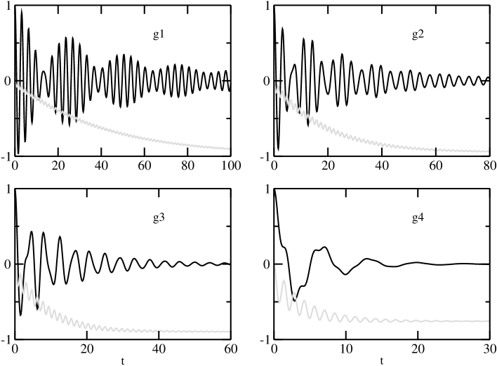
Figure 3: Time evolution of $J_{z}$ (black line) and $J_{x}$ (grey line) for different interaction strengths with the environment ($J\!=\!1$, $\varepsilon\!=\!0$, $\omega_{c}\!=\!50T_{c}$, and $k_{B}T\!=\!0$).

The beat pattern in the dynamics of $J_{z}$ is solely caused by nonresonant bosons. They lead to different corrections to the eigenenergies of the spin, lifting the equidistance of the spectrum. We consider a spin one with zero bias at zero temperature, the same parameters as used in Fig. 3. The three eigenstates of the unperturbed spin labeled in the following by $\left|+\right\rangle$, $\left|0\right\rangle$, and $\left|-\right\rangle$ have the eigenenergies $2T_{c}$, 0, and $-2T_{c}$, respectively. The expectation value of $J_{z}$ becomes $\left\langle J_{z}\right\rangle\!=\!\cos(2T_{c}t)$. The nonresonant bosons of the environment lead to corrections to these eigenenergies. In second order perturbation theory, we find

$$E_{\left|\pm\right\rangle}^{(2)}=-\frac{1}{2}\;\mathchoice{{\vbox{\hbox{$\textstyle-$}}\kern-4.86108pt}}{{\vbox{\hbox{$\scriptstyle-$}}\kern-3.25pt}}{{\vbox{\hbox{$\scriptscriptstyle-$}}\kern-2.29166pt}}{{\vbox{\hbox{$\scriptscriptstyle-$}}\kern-1.875pt}}\!\int_{0}^{\infty}\!d\omega\,\rho(\omega)\,\frac{1}{\omega\mp 2T_{c}}\,,\qquad E_{\left|0\right\rangle}^{(2)}=E_{\left|+\right\rangle}^{(2)}+E_{\left|-\right\rangle}^{(2)}\,.$$ (10)

As a consequence, the three states are not equidistant anymore. The resonant bosons, $\omega_{q}\!=\!2T_{c}$, are neglected in this calculation. They lead to an imaginary part in the energies resulting in damping, which is not our concern at this stage. The next step is to determine the effect of the corrections on the dynamics of $J_{z}$. Neglecting the corrections to the eigenstates themselves yields

$$\left\langle J_{z}\right\rangle_{t}=\cos(\omega_{0}t)\cos(\omega_{b}t)$$ (11)

with $\omega_{0}$ and $\omega_{b}$ defined as

$$\omega_{0}=2T_{c}+\frac{1}{2}\,\big{(}E_{\left|+\right\rangle}^{(2)}-E_{\left|-\right\rangle}^{(2)}\big{)},\qquad\omega_{b}=-\frac{1}{2}\,E_{\left|0\right\rangle}^{(2)}.$$ (12)

As a result, the oscillation frequency $\omega_{0}$ is slightly changed with respect to the unperturbed case and we find indeed a beat pattern with frequency $\omega_{b}$. For an ohmic dissipation, the beat frequency becomes

$$\omega_{b}=\alpha\,\omega_{c}+\alpha\,T_{c}\Big{[}\,e^{2T_{c}/\omega_{c}}\,{\rm Ei}\Big{(}\frac{-2T_{c}}{\omega_{c}}\Big{)}-e^{-2T_{c}/\omega_{c}}\,{\rm Ei}\Big{(}\frac{2T_{c}}{\omega_{c}}\Big{)}\,\Big{]},$$ (13)

where ${\rm Ei}(x)$ denotes the exponential integral. The term in the brackets is of the order of $T_{c}/\omega_{c}$. Hence, for $\omega_{c}\gg T_{c}$, the beat frequency is given in good approximation by $\omega_{b}\!=\!\alpha\omega_{c}$. For weak interactions, the resulting dynamics is in excellent agreement with the numerical solution of the master equation. Naturally, equation (11) does not include damping since dissipative effects of the resonant bosons are not considered in the derivation. The occurrence of a beat pattern is not restricted to the parameters chosen in this example. Similar patterns are equally found for larger spins, $J\!>\!1$, and finite temperatures. The pattern dissolves at high temperatures or high spins. Even for a finite bias, $\varepsilon\!>\!0$, such patterns can be observed.

7 Conclusion

The collective character of the model becomes visible for larger spins where we found a superradiance-like decay of the $z$-component of the spin, the time scale of which decreases with increasing spin size. The beat pattern in the dynamics of $J_{z}$ for intermediate spins is caused by the nonresonant bosons of the environment. We conjecture that the beat pattern is a characteristic property of an intermediate spin with weak dissipation.

In our study of a large spin coupled to a dissipative environment, the theoretical description applied to real spins as well as to dissipation-induced collective effects in pseudo-spin systems such as ensembles or arrays of two-level systems. We derived a master equation for arbitrary spin $J$ within the Born-Markov approximation. When comparing our results for $J\!=\!1/2$ and ohmic dissipation to standard spin-boson NIBA (and beyond) calculations [1], we found good agreement at all temperatures and arbitrary parameter values, as long as the dissipative coupling is weak. We conclude that the master equation in Born-Markov approximation is a reliable method to describe the physics in the weak coupling limit.

References

- [1] U. Weiss, Quantum Dissipative Systems (World Scientific, Singapore, 1999).
- [2] A. J. Leggett, S. Chakravarty, A. T. Dorsey, M. P. A. Fisher, A. Garg, and W. Zwerger, Rev. Mod. Phys. 59, 1 (1987).
- [3] S. Kronmüller, W. Dietsche, K. v. Klitzing, G. Denninger, W. Wegscheider, and M. Bichler, Phys. Rev. Lett. 82, 4070 (1999); J. H. Smet, R. A. Deutschmann, F. Ertl, W. Wegscheider, G. Abstreiter, and K. v. Klitzing, Nature 415, 281 (2002).
- [4] W. Apel and Yu. A. Bychkov, Phys. Rev. Lett. 82, 3324 (1999); Phys. Rev. B 63, 224405 (2001).
- [5] R. Sessoli, D. Gatteschi, A. Caneschi, and M. A. Novak, Nature 365, 141 (1993).
- [6] W. Wernsdorfer and R. Sessoli, Science 284, 133 (1999).
- [7] A. Schmid, Phys. Rev. Lett. 51, 1506 (1983).
- [8] F. Guinea, V. Hakim, and A. Muramatsu, Phys. Rev. Lett. 54, 263 (1985).
- [9] M. P. A. Fisher and W. Zwerger, Phys. Rev. B 32, 6190 (1985).
- [10] M. Thorwart, M. Grifoni, and P. Hänggi, Phys. Rev. Lett 85, 860 (2000).
- [11] M. Thorwart, M. Grifoni, and P. Hänggi, Ann. Phys. 293, 15 (2001).
- [12] T. Vorrath, T. Brandes, and B. Kramer, in Recent Progress in Many-Body Theories, edited by R. Bishop, T. Brandes, K. Gernoth, N. Walet, and Y. Xian (World Scientific, Singapore, 2002), p. 487.
- [13] R. H. Dicke, Phys. Rev. 93, 99 (1954).
- [14] H. Carmichael, An Open Systems Approach to Quantum Optics (Springer-Verlag, Berlin, 1993).
- [15] D. Loss and D. P. DiVincenzo, cond-mat/0304118.
- [16] L. Hartmann, I. Goychuk, M. Grifoni, and P. Hänggi, Phys. Rev. E 61, R4687 (2000).
- [17] R. K. Wangsness and F. Bloch, Phys. Rev. 89, 728 (1953).
- [18] F. Bloch, Phys. Rev. 105, 1206 (1957).
- [19] M. Gross and S. Haroche, Phys. Rep. 93, 301 (1982).