Quantum chaos and random matrix theory for fidelity decay
in quantum computations with static imperfections

Abstract

We determine the universal law for fidelity decay in quantum computations of complex dynamics in presence of internal static imperfections in a quantum computer. Our approach is based on random matrix theory applied to quantum computations in presence of imperfections. The theoretical predictions are tested and confirmed in extensive numerical simulations of a quantum algorithm for quantum chaos in the dynamical tent map with up to 18 qubits. The theory developed determines the time scales for reliable quantum computations in absence of the quantum error correction codes. These time scales are related to the Heisenberg time, the Thouless time, and the decay time given by Fermi’s golden rule which are well known in the context of mesoscopic systems. The comparison is presented for static imperfection effects and random errors in quantum gates. A new convenient method for the quantum computation of the coarse-grained Wigner function is also proposed.

1 Introduction

Recently a great deal of attention has been attracted to the problem of quantum computation (see e.g. josza ; steane ; chuang ). A quantum computer is viewed as a system of qubits. Each qubit can be considered as a two-level quantum system, e.g. one-half spin in a magnetic field. For $n_{q}$ qubits the whole system is characterized by a finite - dimensional Hilbert space with $N\;=\;2^{n_{q}}$ quantum states. It has been shown that all unitary operations in this space can be realized with elementary quantum gates which include one-qubit rotations $B^{(1)}$ and two-qubit controlled operations,   e.g.   controlled-NOT gate $C^{(N)}$ or controlled phase-shift gates $B^{(2)}(\phi)$ (see e.g. chuang ; divi ). The gates $C^{(N)}$ and $B^{(2)}(\phi)$ assume that the interaction between qubits can be switched on and off in a controllable way with sufficiently high accuracy. Various computational algorithms in the space $N$ can be represented as a sequence of elementary gates. A general unitary operation (unitary matrix) in this space requires an exponential ( in $n_{q}$) number of elementary gates. However, there are important examples of algorithms for which the quantum computation can be performed with a number of operations (gates) much smaller than with the classical algorithms. The most famous is the Shor algorithm for factorization of integers with $n_{q}$ digits which on a quantum computer can be performed with $O(n_{q}^{3})$ gates contrary to an exponential number of operations required for any known classical algorithm shor . Another example is the Grover algorithm for a search of unstructured database which has a quadratic speedup comparing to any classical algorithm grover .

A quantum computation can be much faster than a classical one due the massive parallelism of many-body quantum mechanics since any step of a quantum evolution is a multiplication of a vector by a unitary matrix. A very important example is the quantum Fourier transform (QFT) which can be performed for a vector of size $N=2^{n_{q}}$ with $O({n_{q}}^{2})$ gates instead of $O(n_{q}2^{n_{q}})$ classical operations required for the fast Fourier transform (FFT) (see e.g. josza ; chuang ). With the help of QFT the quantum evolution of certain many-body quantum systems can be performed in a polynomial number of gates lloyd ; ortiz . Another example can be found in the evolution of quantum dynamical systems which are chaotic in the classical limit (see e.g. chirikov ; izrailev ). Such systems are described by chaotic quantum maps and include the quantum baker map schack , the quantum kicked rotator georgeotkr , the quantum saw-tooth map benentist and the quantum double-well map well . For them a map iteration can be performed for $N$-size vector in $O({n_{q}}^{2})$ or $O({n_{q}}^{3})$ gates while a classical algorithm would need $O(n_{q}2^{n_{q}})$ operations. This however does not necessary lead to an exponential gain since the final step with extraction of information by measurements also should be taken into account. Thus, for example, the quantum simulation of the Anderson metal-insulator transition gives only a quadratic speedup even if each step of quantum evolution is performed in a polynomial number of gates pomeransky . Among other algorithms, let us refer to the quantum computation of classical chaotic dynamics where some new information can be obtained efficiently cat ; stratt .

The main obstacle to experimental implementation of a quantum computer is believed to be decoherence induced by unavoidable couplings to external world (see e.g. zurek ). However, even if we imagine that there are no external couplings there still remains internal static imperfections inside a quantum computer. These static imperfections generate residual couplings between qubits and variation of energy level-spacing from one qubit to another. As it was shown in georgeot such imperfections lead to emergence of many-body quantum chaos in a quantum computer hardware if a coupling strength exceeds a quantum chaos threshold. In a realistic quantum computer this threshold drops only inversely proportionally to the number of qubits $n_{q}$ while the energy spacing between nearby levels drops exponentially with $n_{q}$. The dependence of this threshold on quantum computer parameters was studied analytically and numerically by different groups georgeot ; flambaum ; berman ; benentieu ; braun The time scales for onset of quantum chaos were also determined.

It is of primary importance to understand how effects of external decoherence and internal static imperfections affect the accuracy of quantum computations. A very convenient characteristic which allows to analyze these effects is the fidelity $f$ of quantum computation. It is defined as $f(t)=|<\psi_{\varepsilon}(t)|\psi(t)>|^{2}$ where $|\psi(t)>$ is the quantum state at time $t$ computed with perfect (or ideal) gates, while $|\psi_{\varepsilon}(t)>$ is the quantum state at time $t$ computed with imperfect gates characterized by an imperfection strength $\varepsilon$. If the fidelity is close to unity then a quantum computation with imperfections is close to the ideal one while if $f$ is significantly smaller than 1 then the computation gives, generally, wrong results.

At first the fidelity was used to characterize the effects of perturbation on quantum evolution in the regime of quantum chaos peres . Indeed, for the classical chaotic dynamics the small errors grow exponentially with time while for the quantum evolution in the regime of quantum chaos small quantum errors only weakly affect the dynamics. For example, the time reversibility is broken by small errors for classical chaotic dynamics while it is preserved for the corresponding quantum dynamics in presence of small quantum errors dls1983 ; casati1986 . In the context of quantum computation the qualitative difference between classical and quantum errors is analyzed in cat . Recently, the interest to the fidelity decay induced by perturbations of dynamics in the regime of quantum chaos has been renewed pastawski ; beenakker ; veble ; como ; prosen ; cohen ; cerruti ; adamov . It has been shown that the rate $\Gamma$ of exponential decrease of $f$ is given by the Fermi golden rule for small perturbations while for sufficiently strong perturbations the decay rate is determined by the Kolmogorov-Sinai entropy related to the Lyapunov exponent of classical chaotic dynamics beenakker ; veble . For small perturbations the fidelity decay can be expressed with the help of correlation function of quantum dynamics that allows to understand various peculiarities of the decay prosen .

Until recently the fidelity decay and accuracy of quantum computations have been mainly analyzed for the case of random noise errors in the quantum gates paz ; cat ; benentist ; well ; wavelet ; bettelli . Quite naturally in this case the rate of fidelity decay is proportional to the square of error amplitude $\varepsilon$ ($\Gamma\propto\varepsilon^{2}$). Indeed, a random error of amplitude $\varepsilon$ transfers a probability of order $\varepsilon^{2}$ from the ideal state to all other states and as a result the fidelity remains close to unity (within e.g. 10% accuracy) during a time scale $t_{f}\sim 1/(\varepsilon^{2}n_{g})$. Here $n_{g}$ is the number of gates per one map iteration and for polynomial algorithms $n_{g}\sim n_{q}^{\gamma}$ (e.g. for the quantum saw-tooth map $\gamma=2$ benentist ).

Contrary to the case of random errors the effects of static imperfections on fidelity decay have been studied only in benentist ; wavelet . The numerical simulations performed there with up to 18 qubits show that for small strength of static imperfections $\varepsilon$ the time scale $t_{f}$ varies as $t_{f}\sim 1/(\varepsilon n_{g}\sqrt{n_{q}})$. Such a dependence implies that in the limit of small $\varepsilon$ the effects of static imperfections dominate the fidelity decay comparing to the case of random errors benentist ; wavelet . Simple estimates based on the Rabi oscillations have been proposed to explain the above dependence extracted from numerical data benentist ; wavelet .

Since the numerical results show that the static imperfections lead to a more rapid fidelity decay, compared to random errors fluctuating from gate to gate, it is important to investigate their effects in more detail. This is the aim of this paper in which we carry out extensive numerical and analytical studies of static imperfections effects on fidelity decay using as an example a quantum algorithm for the quantum tent map which describes dynamics in a mixed phase space with chaotic and integrable motion. For the case when the algorithm describes the dynamics in the regime of quantum chaos a scaling theory for universal fidelity decay is developed on the basis of the random matrix theory (RMT) dyson ; mehta ; guhr . This theory is tested in extensive numerical simulations with up to 18 qubits and the obtained results confirm its analytical predictions which are rather different from the conclusions of the previous studies benentist ; wavelet . We also investigate the regime of fidelity decay for integrable quantum dynamics where the situation happens to be more complicated. In addition, a simple quantum algorithm is proposed for approximate computation of the coarse-grained Wigner function (the Husimi function) wigner ; husimi and its stability in respect to imperfections is tested on the example of quantum tent map.

It is important to note that all quantum operations required for implementation of the quantum tent map have been already realized for 3 - 7 qubits in the NMR-based quantum computations reported in Refs. chuang1 ; cory . An efficient measurement procedure for fidelity decay in quantum computations is proposed in emerson .

The paper is organized as follows. In Sec. 2 we describe the classical and quantum tent map. The algorithm for quantum dynamics is derived in Sec. 3. The fidelity decay for random errors in quantum gates is analyzed in Sec. 4. The analytical theory for fidelity decay induced by static imperfections is developed on the basis of RMT approach in Sec. 5. This theory is tested in extensive numerical simulations presented in Sec. 6. An approximate algorithm for the quantum computation of the Husimi function is studied in Sec. 7. The conclusion is given in Sec. 8.

2 Classical and quantum tent map

We consider a kicked rotator whose dynamics is governed by the time dependent Hamiltonian,

$$H(t)=\frac{Tp^{2}}{2}+V(\theta)\sum_{m=-\infty}^{\infty}\delta(t-m)$$ (1)

with the potential of kick

$$V(\theta)=\left\{\begin{array}[]{ll}-\frac{k}{2}\theta(\theta-\pi)&,\quad 0\leq\theta<\pi\\ \frac{k}{2}(\theta-\pi)(\theta-2\pi)&,\quad\pi\leq\theta<2\pi\\ \end{array}\right.$$ (2)

where $\theta$ is taken modulo $2\pi$ and $\delta(t)$ is a $\delta$-function, $m$ is an integer. The parameter $k$ determines the kick strength and $T$ gives the rotation of phase between kicks. It is easy to see that the classical evolution for a finite time step $t\to t+1$ with respect to the Hamiltonian (1) can be described by the map,

$$\bar{p}=p-V^{\prime}(\theta)\quad,\quad\bar{\theta}=\theta+\bar{p}\,T\;(\texttt{\ mod\ }2\pi)\quad.$$ (3)

Here bars mark new values of the dynamical variables after one map iteration. This map is similar in structure to the Chirikov standard map chirikov79 . The derivative of the kick-potential,

$$V^{\prime}(\theta)=\left\{\begin{array}[]{ll}k(\frac{\pi}{2}-\theta)&,\quad 0\leq\theta<\pi\\ k(-\frac{3\pi}{2}+\theta)&,\quad\pi\leq\theta<2\pi\\ \end{array}\right.\ ,$$ (4)

has a tent form and is continuous but not differentiable at $\theta=0$ and $\theta=\pi$. This is an intermediate case between the standard map chirikov79 with a perfectly smooth kick-potential and the saw-tooth map benentist with a non-continuous potential.

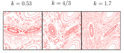
Figure 1: Classical Poincaré sections of the map (3) in ($\theta$, $p$) plane for $T=1$ and $K=k=0.53$, $K=k=4/3$ and $K=k=1.7$.

The dynamics of the classical tent map (3) depends only on one dimensionless parameter $K=kT$, its properties have been studied in tent ; vecheslavov . For small values of $K$ the dynamics is governed by a KAM-scenario with the Kolmogorov-Arnold-Moser (KAM) invariant curves and a stable island at $\theta=3\pi/2$, $p=0$ and a chaotic layer around separatrix starting from the unstable fixed point (saddle) at $\theta=\pi/2$, $p=0$. At $K=4/3$, the last invariant curve is destroyed and one observes a transition to global chaos with a mixed phase space containing big regions with regular dynamics tent ; vecheslavov .

In Fig. 1, the Poincaré sections of the map (3) for the three values $K=0.53,\ 4/3,\ 1.7$ are shown. Here we have replaced $p$ by its value modulo $2\pi/T$ which is appropriate since the classical map is invariant with respect to the shift $p\to p+2\pi/T$. Fig. 1 confirms the above scenario of a transition to global chaos at $K=4/3$. In the following, we are particularly interested in a typical case $K=1.7$, which exhibits global chaos with quite large stable islands in phase space related to the main and secondary resonances.

At $K\geq 4$, the phase space becomes completely chaotic and the dynamics is characterized by a diffusive growth in $p$. The diffusion rate $D$ in $p$ can be obtained with the help of random phase approximation that gives

$$\langle(p-p_{0})^{2}\rangle\approx D\,t\quad,\quad D=\langle V^{\prime}(\theta)^{2}\rangle_{\theta}=\frac{\pi^{2}}{12}\,k^{2}\ .$$ (5)

Here and below $t$ is an integer which gives the number of map iterations (kicks).

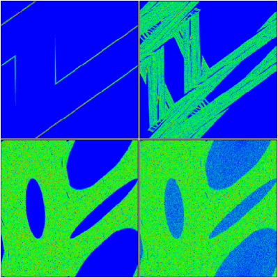
Figure 2: Density plots of the Husimi functions (see below Sec. 7) of the quantum state $|\psi(t){>}$ for $t=5$ (top left panel), $t=15$ (top right panel) and $t=5625$ (bottom left panel) with an initial state $|\psi(0){>}$ chosen as a minimal coherent (gaussian) wave packet closely located to the saddle at $\theta=\pi/2$, $p=0$. The bottom right panel corresponds to the quantum state after 5625 iterations computed on a quantum computer with static imperfections for $\varepsilon=7\cdot 10^{-7}$, here the fidelity is $f=0.9388$ (see below Secs. 3,6 for details). The density is minimal for blue/black and maximal for red/white. All panels correspond to $n_{q}=16$ qubits, i.e. to a finite dimensional Hilbert space of dimension $N=2^{16}$, $T=2\pi/N$.

The quantum dynamics of the Hamiltonian (1) is given by the Schrödinger equation,

$$i\frac{\partial}{\partial t}|\psi(t){>}=H(t)\,|\psi(t){>}\ .$$ (6)

Here in the Hamiltonian $H(t)$ the variables $\hat{p}$ and $\hat{\theta}$ are operators with the commutator $[\hat{p},\hat{\theta}]=-i$. They have integer eigenvalues $p$ for $\hat{p}$ and real eigenvalues $\theta$ in the interval $[0,2\pi[$ for $\hat{\theta}$. As in the classical case one can determine the evolution for one map iteration:

$$|\psi(t+1){>}=U\,|\psi(t){>}=e^{-iT\hat{p}^{2}/2}\,e^{-iV(\hat{\theta})}\,|\psi(t){>}\;.$$ (7)

Eq. (7) corresponds to the quantized version of the classical map (3) and defines a quantum map that can be efficiently simulated on a quantum computer. Here $\hbar=1$ and the quasiclassical limit correspond to $T\to 0$, $k\to\infty$ with $K=kT=const$.

For quantum dynamics we concentrate our studies on the case $K=kT=1.7$ and $T=2\pi/N$ that corresponds to evolution on one classical cell (see Fig. 1) with $N$ quantum states. As an initial state we use a minimal coherent wave packet corresponding to a given $N$ which is placed in a chaotic or integrable component (near the unstable or stable fixed point at $p=0,\theta=\pi/2$ or $\theta=3\pi/2$). An example of the Husimi function (see Sec. 7) for a chaotic case is shown in Fig. 2 for different moments.

3 Quantum algorithm

The quantum map (7) can be simulated on a quantum computer in a polynomial number of gates. The quantum algorithm has similarities with those described in georgeotkr ; benentist . To perform one iteration of the quantum map (7) we represent the states $|\psi{>}$ by a quantum register with $n_{q}$ qubits. In particular, the eigenstates $|p{>}$ of the momentum operator are identified with the quantum-register states

$$|\alpha_{0},\alpha_{1},\ldots,\alpha_{n_{q}-1}{>}=|\alpha_{0}{>}_{0}\,|\alpha_{1}{>}_{1}\,\ldots\,|\alpha_{n_{q}-1}{>}_{n_{q}-1}$$ (8)

where $\alpha_{j}=0$ or $1$ and

$$p=\sum_{j=0}^{n_{q}-1}\alpha_{j}\,2^{j}\ .$$ (9)

The states $|0{>}_{j}$ and $|1{>}_{j}$ correspond to the two basis states of the $j-$th qubit. Obviously, this representation introduces a Hilbert space of finite dimension $N=2^{n_{q}}$; the operator $\hat{p}$ has the eigenvalues: $p=0,\ldots,N-1$.

A quantum computer is a machine that is able to prepare a quantum register with a well defined initial condition and to perform certain well controlled unitary operations on this quantum register. These particular operations are called quantum gates and one typically assumes that the quantum computer can be constructed with quantum gates that manipulate at most two qubits. Here we use as elementary gates the phase-shift gates $B_{j}^{(1)}$ and controlled phase-shift gates $B_{jk}^{(2)}$:

$$B_{j}^{(1)}(\phi)\,|p{>} = e^{i\alpha_{j}\phi}\,|p{>}\quad,$$ (10)

$$B_{jk}^{(2)}(\phi)\,|p{>} = e^{i\alpha_{j}\alpha_{k}\phi}\,|p{>}\quad,\quad j\neq k\quad$$ (11)

where $p$ is of the form (9). These gates provide a phase factor $e^{i\phi}$ if $\alpha_{j}=1$ for the simple phase-shift or if $\alpha_{j}=\alpha_{k}=1$ for the controlled phase-shift. Using Eq. (9), one easily verifies that the momentum dependent factor of the unitary operator $U$ in (7) can be expressed in terms of these gates by:

$$e^{-iT\hat{p}^{2}/2}=\prod_{j<k}^{n_{q}-1}B_{jk}^{(2)}(-T\,2^{j+k})\prod_{j=0}^{n_{q}-1}B_{j}^{(1)}(-T\,2^{2j-1})\ .$$ (12)

The situation is different for the phase factor containing the kick-potential since this factor is not diagonal in momentum representation. It is therefore necessary to transform to the basis of eigenstates of the operator $\hat{\theta}$. For this, following josza we consider the unitary operator $U_{\rm QFT}$ defined by:

$$U_{\rm QFT}\,|p{>}=\frac{1}{\sqrt{N}}\sum_{\tilde{p}=0}^{N-1}e^{2\pi i\,p\,\tilde{p}/N}\,|\tilde{p}{>}\ .$$ (13)

Then the eigenstates of $\hat{\theta}$ with eigenvalues $\theta=\frac{2\pi p}{N}$ are simply given by: $U_{\rm QFT}^{-1}\,|p{>}$ and more generally the operators $\hat{\theta}$ and $\hat{p}$ are related by:

$$\hat{\theta}=U_{\rm QFT}^{-1}\ \left(\frac{2\pi\,\hat{p}}{N}\right)\ U_{\rm QFT}\ .$$ (14)

Using Eqs. (2), (9) and (14) it is straight-forward to show that the unitary factor of $U$ containing the kick-potential can be written as:

$$e^{-iV(\hat{\theta})} = U_{\rm QFT}^{-1}\prod_{j<k}^{n_{q}-2}\Bigl{\{}B_{j,k,n_{q}-1}^{(3)}(-k\pi^{2}\,2^{j+k-2n_{q}+3})$$

$$\times\quad B_{jk}^{(2)}(k\pi^{2}\,2^{j+k-2n_{q}+2})\Bigr{\}}$$

$$\times\prod_{j=0}^{n_{q}-2}\Bigl{\{}B_{j,n_{q}-1}^{(2)}(-k\pi^{2}\,2^{j-n_{q}+2}(2^{j-n_{q}+1}-1))$$

$$\times\quad B_{j}^{(1)}(k\pi^{2}\,2^{j-n_{q}}(2^{j-n_{q}+1}-1))\Bigr{\}}\ U_{\rm QFT}\ .$$

Here we have used a three-qubit gate for a controlled-controlled phase-shift defined by (cf. Eqs. (10), (11)):

$$B_{jkl}^{(3)}(\phi)\,|p{>}=e^{i\alpha_{j}\alpha_{k}\alpha_{l}\phi}\,|p{>}\quad.$$ (16)

In Eq.(3) it appears for $l=n_{q}-1$ because of the two distinct cases in Eq.(2). In principle, this gate is not directly available in the set of one- and two-qubit gates used for a quantum computer. However, it can be constructed from 5 two-qubit gates by:

$$B_{jkl}^{(3)}(\phi)=B_{jl}^{(2)}\left(\frac{\phi}{2}\right)\,B_{jk}^{(2)}\left(\frac{\phi}{2}\right)\,C^{(N)}_{kl}\,B_{jk}^{(2)}\left(-\frac{\phi}{2}\right)\,C^{(N)}_{kl}$$ (17)

where $C^{(N)}_{kl}$ is the controlled-not gate that exchanges the states $|0>_{k}$ and $|1>_{k}$ for the $k$-th qubit if $\alpha_{l}=1$. In matrix representation it is given by:

$$C^{(N)}_{kl}=\left(\begin{array}[]{cccc}1&0&0&0\\ 0&1&0&0\\ 0&0&0&1\\ 0&0&1&0\\ \end{array}\right)$$ (18)

where the index $\alpha_{l}$ corresponds to the outer block structure and $\alpha_{k}$ to the inner block structure.

Following the description josza , the QFT operator $U_{\rm QFT}$ can be written in the form:

$$U_{\rm QFT}^{\pm 1}=R\ \prod_{j=0}^{n_{q}-1}\Bigl{\{}A_{j}\prod_{k=j+1}^{n_{q}-1}B_{jk}^{(2)}(\pm\pi\,2^{j-k})\Bigr{\}}$$ (19)

where $R$ is the unitary operator that reverses the order of the qubits and $A_{j}$ is a one-qubit gate with the matrix representation:

$$A_{j}=\frac{1}{\sqrt{2}}\left(\begin{array}[]{cc}1&1\\ 1&-1\\ \end{array}\right)\ .$$ (20)

We note that in the outer product in Eq.(19) the factors are ordered from left to right with increasing $j$.

Combining, Eqs.(12), (3) and (19), we see that the quantum map (7) can be expressed by a total number of $n_{g}=\frac{9}{2}n_{q}^{2}-\frac{11}{2}n_{q}+4$ elementary quantum gates (and 2 $R$-operations). On a classical computer one iteration of the quantum tent map requires $O(n_{q}2^{n_{q}})$ operations coming mainly from the FFT.

To investigate the stability of the quantum algorithm for the tent map we consider two models of imperfections. The first model represents the random errors in quantum gates fluctuating in time from one gate to another (random noise errors). In this case for all phase-shift gates we replace $\phi$ by $\phi+\delta\phi$ with random $\delta\phi\in[-\varepsilon,\,\varepsilon]$ that is different for each application of the gate. For the gates containing the Pauli matrix $\sigma_{x}$ we replace it by $\vec{n}\cdot\vec{\sigma}$ where $\vec{n}$ is a random unit-vector close to $\vec{e}_{x}$ with $|\vec{n}-\vec{e}_{x}|\leq\varepsilon$.

The second model describes only static imperfections and is similar to one used in georgeot ; benentist ; wavelet ; pomeransky . In this case the effect of static imperfections is modeled by an additional unitary rotation between two arbitrary gates which has the form : $U_{s}=e^{i\delta H}$. Here the Hamiltonian $\delta H$ is given by:

$$\delta H=\sum_{j=0}^{n_{q}-1}\delta_{j}\,\sigma_{j}^{(z)}+2\sum_{j=0}^{n_{q}-2}J_{j}\,\sigma_{j}^{(x)}\,\sigma_{j+1}^{(x)}$$ (21)

where $\sigma_{j}^{(\nu)}$ are the Pauli matrices acting on the $j$th qubit and $\delta_{j},\,J_{j}\in[-\sqrt{3}\varepsilon,\,\sqrt{3}\varepsilon]$ are random coefficients which are drawn only once at the beginning and kept fixed during the simulation. These coefficients determine one disorder realization. In addition to a linear chain of qubits we also analyzed a case with qubits distributed on a square lattice which gave qualitatively similar results (see Sec. 6).

4 Quantum computation with random errors

The numerical results for fidelity decay induced by random errors in quantum gates are presented in Fig. 3. They clearly show that the decrease is exponential with time $t$ and is given by the fit:

$$f(t)=\exp(-t/t_{r})\;;\ t_{r}=1/(0.095\varepsilon^{2}n_{q}^{2})\approx 47/(\varepsilon^{2}n_{g})\;.$$

As discussed in the introduction, the decay rate per gate is proportional to $\varepsilon^{2}$ since on each step noise transfer such a probability from an ideal state to all other states (see paz ; cat ; benentist ; well ; wavelet ; bettelli ). With a few percent accuracy the numerical constant in (4) is close to the lower bound discussed in bettelli .

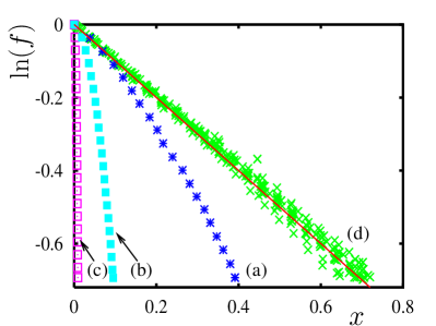
Figure 3: Data points (d) represent the fidelity decay for the case of random noise errors in the gates of quantum algorithm. The fidelity $f=|{<}\psi(t)|\psi_{\rm noise}(t){>}|^{2}$ is shown as a function of the scaling variable $x=0.095\,t\,\varepsilon^{2}\,n_{q}^{2}$ with $n_{q}=10,12,14,16$ and $0.001\leq\varepsilon\leq 0.1$. The full line corresponds to the function $f=\exp(-x)$. Data points (a), (b) and (c) represent the fidelity decay ($f=|{<}\psi(t)|\psi_{\rm stat}(t){>}|^{2}$) as a function of the scaling variable $x=t\,\varepsilon^{2}\,n_{q}n_{g}^{2}$ for the case of static imperfections with $n_{q}=10$, $n_{g}=\frac{9}{2}n_{q}^{2}-\frac{11}{2}n_{q}+4$ being the number of elementary gates for one application of the quantum map and with (a) $\varepsilon=3\cdot 10^{-5}$, (b) $\varepsilon=6\cdot 10^{-6}$ and (c) $\varepsilon=5\cdot 10^{-7}$. The scaling variable $x$ corresponds in all cases to $\Gamma t$ where $\Gamma$ is the decay rate obtained from Fermi’s golden rule. Therefore, the data curves (a), (b), (c) are tangent to $\exp(-x)$ for small $x$. The number of shown data points has been strongly reduced in order to increase the visibility of the different symbols. (same approach is used for other figures). Here and in Figs. 4-8, the initial state is as in Fig. 2, $K=1.7$, $T=2\pi/N$.

While with random errors the fidelity drops by a significant amount in a purely exponential way the situation in the case of static imperfections is more complicated (see Fig. 3). In this case the initial exponential decrease is followed by a gaussian exponential one. As a result static imperfections give a faster decay of fidelity. The transition between these two types of decay depends on the strength of imperfections $\varepsilon$. Moreover, in scaled variables the weaker is $\varepsilon$ the stronger is the gaussian decrease of fidelity (see Fig 3). We shall describe these phenomenon using the following RMT approach.

5 Quantum computation with static imperfections: RMT approach

Let us denote by $\tilde{U}$ the unitary operator for the quantum map with static imperfections and by $U$ the unitary operator for the ideal quantum map. We denote by $U_{j}$, $j=1,\ldots,n_{g}$ the elementary quantum gates which constitute the quantum map. According to the description of the quantum algorithm in section 3 we write :

$$U=U_{n_{g}}\cdot\ldots\cdot U_{2}\cdot U_{1}$$ (22)

and

$$\tilde{U}=U_{n_{g}}\cdot e^{i\delta H}\cdot\ldots\cdot U_{2}\cdot e^{i\delta H}\cdot U_{1}\cdot e^{i\delta H}$$ (23)

where $\delta H$ is the hermitian operator describing the static imperfections. In numerical simulations we have used the particular expression (21) for $\delta H$ but we mention that our approach does not rely on this expression and is much more general. We now introduce an effective perturbation operator for the full quantum map by: $\tilde{U}=U\,e^{i{\delta H_{\rm eff}}}$. The operator ${\delta H_{\rm eff}}$ is determined by:

$$e^{i{\delta H_{\rm eff}}}=e^{i\delta H(n_{g}-1)}\cdot\ldots\cdot e^{i\delta H(1)}\cdot e^{i\delta H}$$ (24)

with

$$\delta H(j)=U_{j-1}^{-1}\cdot\ldots\cdot U_{1}^{-1}\ \delta H\ U_{1}\cdot\ldots\cdot U_{j-1}\ .$$ (25)

We mention that the precise relation between ${\delta H_{\rm eff}}$ and $\delta H$ is not important for the following argumentation and we will need only one characteristic time scale $t_{c}$ defined by:

$$\frac{1}{t_{c}}=\frac{1}{N}{\texttt{tr}}\left({\delta H_{\rm eff}}^{2}\right).$$ (26)

We furthermore assume that ${\texttt{tr}}({\delta H_{\rm eff}})=0$ (the case of ${\texttt{tr}}({\delta H_{\rm eff}})\neq 0$ can be trivially transformed to the this case prosen and $\delta H$ in Eq. (21) has actually a vanishing trace).

Following Ref. prosen , we express the fidelity in terms of a correlation function of the perturbation. For this we write the fidelity at time $t$ as $f(t)=|A(t)|^{2}$ with the amplitude:

$$A(t) = \left\langle U^{-t}\left(Ue^{i{\delta H_{\rm eff}}}\right)^{t}\right\rangle_{Q}$$

$$= \left\langle e^{i{\delta H_{\rm eff}}(t-1)}\cdot\ldots\cdot e^{i{\delta H_{\rm eff}}(1)}\cdot e^{i{\delta H_{\rm eff}}(0)}\right\rangle_{Q}$$

and

$${\delta H_{\rm eff}}(\tau)=U^{-\tau}\ {\delta H_{\rm eff}}\ U^{\tau}\ .$$ (28)

Here $\langle\cdots\rangle_{Q}$ denotes the quantum expectation value. For a fixed initial state $|\psi_{0}{>}$ this expectation value is given by: $\langle\cdots\rangle_{Q}={<}\psi_{0}|\cdots|\psi_{0}{>}$. However, in the following we average over all possible initial states that corresponds to: $\langle\cdots\rangle_{Q}=\frac{1}{N}{\texttt{tr}}(\dots)$. Since we are interested in the case where the fidelity is close to 1 we can expand (5) up to second order in ${\delta H_{\rm eff}}$ (or equivalently in $\varepsilon$) :

$$A(t) \approx 1+i\sum_{\tau=0}^{t-1}\left\langle{\delta H_{\rm eff}}(\tau)\right\rangle_{Q}-\frac{1}{2}\sum_{\tau=0}^{t-1}\left\langle{\delta H_{\rm eff}}^{2}(\tau)\right\rangle_{Q}$$ (29)

$$-\frac{1}{2}\sum_{\tau_{1}=0}^{t-1}\sum_{\tau_{2}=0}^{\tau_{1}-1}\left\langle{\delta H_{\rm eff}}(\tau_{1}){\delta H_{\rm eff}}(\tau_{2})\right\rangle_{Q}\ .$$

Now we introduce the correlation function $C(\tau)$ by:

$$C(\tau_{1}-\tau_{2}) = t_{c}\left\langle{\delta H_{\rm eff}}(\tau_{1}){\delta H_{\rm eff}}(\tau_{2})\right\rangle_{Q}$$

$$= t_{c}\left\langle{\delta H_{\rm eff}}(\tau_{1}-\tau_{2}){\delta H_{\rm eff}}(0)\right\rangle_{Q}$$

and we note that $\left\langle{\delta H_{\rm eff}}(\tau)\right\rangle_{Q}=\frac{1}{N}{\texttt{tr}}({\delta H_{\rm eff}})=0$. Combining Eqs. (26), (29) and (5), we obtain:

$$f(t)\approx 1-\frac{t}{t_{c}}-\frac{2}{t_{c}}\sum_{\tau=1}^{t-1}(t-\tau)\,C(\tau)\ .$$ (31)

This provides the general expression relating the fidelity and the correlation function (5) previously obtained in Ref. prosen .

We now assume that the unitary quantum map $U$ can be modeled by a random matrix drawn from Dyson’s circular orthogonal ($\beta=1$) or unitary ($\beta=2$) ensemble dyson ; mehta ; guhr . As we will see it is useful to express $U$ in terms of its eigenvectors and eigenphases:

$$U=V\,e^{i\hat{\theta}}\,V^{\dagger}\quad,\quad\theta=\left(\begin{array}[]{ccc}\theta_{1}&&\\ &\ddots&\\ &&\theta_{N}\\ \end{array}\right)\ .$$ (32)

The matrix $V$ is either real orthogonal ($\beta=1$) or complex unitary ($\beta=2$). Inserting Eqs. (28), (32) in (5), we obtain:

$$C(\tau)=\frac{t_{c}}{N}{\texttt{tr}}\left(V\,e^{-i\tau\hat{\theta}}\,V^{\dagger}\,{\delta H_{\rm eff}}\,V\,e^{i\tau\hat{\theta}}\,V^{\dagger}\,{\delta H_{\rm eff}}\right)\ .$$ (33)

In the following, we want to evaluate the average of $C(\tau)$ with respect to $U$. We first evaluate the average with respect to the matrix elements of $V$ which gives for $N\gg 1$ :

$$\langle C(\tau)\rangle_{U}=\left(\frac{2}{\beta}-1\right)\frac{1}{N}+\frac{1}{N^{2}}\left\langle\sum_{j,k=1}^{N}e^{i\tau(\theta_{j}-\theta_{k})}\right\rangle_{\theta}\ .$$ (34)

Here we have used that ${\texttt{tr}}({\delta H_{\rm eff}})=0$ and we have replaced ${\texttt{tr}}({\delta H_{\rm eff}}^{2})=N/t_{c}$ according to Eq. (26). We have furthermore neglected corrections of order $1/N^{2}$ which arise from small correlations between matrix elements of $V$ at different positions. We note that in (34) the first term vanishes for $\beta=2$. For $\beta=1$ this term arises from additional contributions (in the $V$-average) because the elements of $V$ are real for this case. The diagonal contributions with $j=k$ in the second term of (34) provide the constant $1/N$ (which simplifies the first term). The average over the non-diagonal contributions with $j\neq k$ can be expressed mehta ; guhr in terms of a double integral over the two-point density for the eigenphases $\theta_{j}$. Since this two-point density is related to the two-point correlation function of the random matrix theory we obtain for $\tau\geq 1$ :

$$\langle C(\tau)\rangle_{U}=\frac{1}{N}\left(\frac{2}{\beta}-b_{2}\left(\frac{\tau}{N}\right)\right)$$ (35)

where

$$b_{2}(\tilde{\tau})=\int_{-\infty}^{\infty}ds\ Y_{2}(s)\,e^{2\pi i\,\tilde{\tau}\,s}$$ (36)

is the “two-level form factor” defined as the Fourier transform of the two-point correlation function $Y_{2}(s)$. The form factor of the Wigner-Dyson ensembles is well known dyson ; mehta ; guhr . For the unitary and orthogonal symmetry class it reads (in the large $N$ limit):

$$\beta = 2\ :\quad b(\tilde{\tau})=\left\{\begin{array}[]{ccc}1-|\tilde{\tau}|&\ \textrm{if}&|\tilde{\tau}|\leq 1\,,\\ 0&\ \textrm{if}&|\tilde{\tau}|>1\,,\\ \end{array}\right.$$ (39)

$$\beta = 1\ :\quad b(\tilde{\tau})=\left\{\begin{array}[]{ccc}1-2|\tilde{\tau}|+|\tilde{\tau}|\ln(2|\tilde{\tau}|+1)&\ \textrm{if}&|\tilde{\tau}|\leq 1\,,\\ -1+|\tilde{\tau}|\ln\left(\frac{2|\tilde{\tau}|+1}{2|\tilde{\tau}|-1}\right)&\ \textrm{if}&|\tilde{\tau}|>1\,.\\ \end{array}\right.$$ (42)

Inserting the average correlation function (35) in (31) and replacing the discrete sum by an integral, we finally obtain the following scaling expression for the fidelity:

$$-\langle\ln f(t)\rangle_{U}\approx\frac{N}{t_{c}}\chi\left(\frac{t}{N}\right)$$ (44)

with

$$\chi(s) = s+\frac{2}{\beta}\,s^{2}+\delta\chi(s)\ ,$$ (45)

$$\delta\chi(s) = -2\int_{0}^{s}d\tilde{\tau}\,(s-\tilde{\tau})\,b_{2}(\tilde{\tau})$$ (46)

where $s=t/N$. Using the random matrix expressions (39), (LABEL:rmt_eq17), we find for $\beta=2$:

$$\delta\chi(s)=\left\{\begin{array}[]{ccc}-s^{2}+\frac{1}{3}s^{3}&\ \textrm{if}&s\leq 1\,,{\phantom{\Big{|}}}\\ -\frac{2}{3}&\ \textrm{if}&s>1\,,{\phantom{\Big{|}}}\\ \end{array}\right.$$ (47)

and for $\beta=1$:

$$\delta\chi(s)=\left\{\begin{array}[]{cc}\left.\begin{array}[]{l}\frac{1}{18}(-3s-24s^{2}+17s^{3})\\ +\frac{1}{12}(1+3s-4s^{3})\ln(2s+1){\phantom{\Big{|}}}\\ \end{array}\right\}&\textrm{if}\ s\leq 1\,,\\ &\\ \left.\begin{array}[]{l}\frac{3}{4}\ln(3)(s-1)-\frac{5}{9}\\ +\frac{1}{3}(2-3s+s^{2}){\phantom{\Big{|}}}\\ +\frac{1}{12}(1-3s+4s^{3})\ln(2s-1)\\ +\frac{1}{12}(1+3s-4s^{3})\ln(2s+1){\phantom{\Big{|}}}\\ \end{array}\right\}&\textrm{if}\ s>1\,.\\ \end{array}\right.\\$$ (48)

Eqs. (44-48) provide the key result of this section. From the practical point of view the contribution of $\delta\chi(s)$ in (45) is not very important, since (for $\beta=1$):

$$\delta\chi(s) \approx -s^{2}+\frac{2}{3}s^{3}\quad(\textrm{if}\quad s\ll 1)\ ,$$ (49)

$$\delta\chi(s) \approx \left(\frac{3}{4}\ln(3)-1\right)\,s+\frac{1}{6}\ln(2s)-\frac{3}{4}\ln(3)+\frac{1}{3}$$

$$\approx -0.17604s+\frac{1}{6}\ln(2s)-0.49063$$

$$\qquad\qquad(\textrm{if}\quad s\gg 1)\ .$$

Therefore for small $s$ the linear term and for large $s$ the quadratic term dominate the behavior of $\chi(s)$ in the expression (45). In the next section we compare this theoretical random matrix result to the numerical data of the fidelity obtained for the quantum version of the tent map.

Before doing so, we want to discuss three particular points. First, we have to evaluate the time scale $t_{c}$ that characterizes the effective strength of the perturbation. From Eqs. (24) and (26), we obtain in lowest order in $\varepsilon$:

$$\frac{1}{t_{c}}=\frac{1}{N}\sum_{j,k=0}^{n_{g}-1}{\texttt{tr}}\Bigl{(}\delta H(j)\delta H(k)\Bigr{)}$$ (51)

with $\delta H(j)$ given by (25). This expression is similar in structure to Eqs. (29) or (31) but with the important difference that here the “time” index corresponds to the number of elementary gates and not to the iteration number of the quantum map. Since the elementary gates affect only one or two qubits (“spins”) the correlation decay between $\delta H(j)$ and $\delta H(k)$ will be quite weak and we can obtain a good estimate of (51) by:

$$\frac{1}{t_{c}}=an_{g}^{2}\frac{1}{N}{\texttt{tr}}(\delta H^{2})\approx an_{g}^{2}\,5\,n_{q}\varepsilon^{2}$$ (52)

where $a<1$ is a numerical constant taking into account the exact correlation decay and the trace has been evaluated using Eq. (21). The numerical results of the next Section indicate clearly that $a\approx 1/5$ such that the overall numerical factor is 1 and we have:

$$t_{c}=\frac{1}{\varepsilon^{2}n_{q}n_{g}^{2}}\quad,\quad n_{g}=\frac{9}{2}n_{q}^{2}-\frac{11}{2}n_{q}+4\ .$$ (53)

The second point to discuss concerns the fact that the phase space is mixed and not completely chaotic. As it can be seen from Fig. 2 the chaotic region fills approximately a fraction of $0.65$ of the full phase space. If the initial state is a gaussian wave packet placed in the chaotic region then its penetration inside the integrable islands induced by quantum tunneling will take exponentially long time scale: $\propto\exp(N)$. Therefore with a good approximation we may say that in absence of imperfections the dynamics takes place only inside the chaotic component. Let us introduce now the Heisenberg time scale $t_{\rm H}=2^{n_{q}}$ which is determined by an average energy level-spacing for $2^{n_{q}}$ quantum levels in the whole phase space. If the whole phase space is chaotic then in the above RMT approach $N=t_{\rm H}$. However, for the case of Fig. 2 the chaotic component covers only a relative fraction $\sigma=0.65$ of the whole phase space. Due to that in the previous RMT expressions we should put $N\approx\sigma t_{\rm H}=0.65\cdot 2^{n_{q}}$ to determine properly the number of chaotic states. As a consequence, the expression (44) now reads ($\beta=1$ for the tent map):

$$-\langle\ln f(t)\rangle_{U}\approx\frac{\sigma\,t_{\rm H}}{t_{c}}\chi\left(\frac{t}{\sigma\,t_{\rm H}}\right)\approx\frac{t}{t_{c}}+\frac{2}{\sigma}\,\frac{t^{2}}{t_{c}t_{\rm H}}\;.$$ (54)

Here we have neglected the contribution of $\delta\chi(s)$.

It is interesting to note that there is a formal analogy between the fidelity decay given by (54) and the decrease of the probability to stay near the origin which has been studied in mesoscopic and RMT systems (see e.g. khmelnitski ; mirlin ; maspero ; sokolov ; frahm ). There, the time scale $t_{c}$ is replaced by the diffusive Thouless time scale $t_{\rm Th}$ and the second term with the Heisenberg time scale has negative sign.

Finally, the third point concerns the fact that the above results are based on the assumption that the quantum evolution given by the exact quantum algorithm can be described by RMT. In particular, we assume that in the dynamical evolution the ergodicity is established very rapidly after a few map iterations. This is correct for the choice $T=2\pi/N$ which corresponds to the dynamics in one classical cell. We note that it is also possible to have many classical cells by the alternative choice $T=2\pi L/N$ with $L\gg 1$ but fixed in the semiclassical limit $N\to\infty$. For $K$ above the global chaos border, the classical dynamics is governed by a diffusive dynamics which covers all cells after the Thouless time scale $t_{\rm Th}\approx N^{2}/D\sim L^{2}/K^{2}$ where $D$ is the diffusion constant given by Eq. (5). In this case the theoretical treatment has to be modified since the matrix $U$ will not be a member of the circular ensemble. However, choosing a static perturbation sufficiently complicated such that it can be modeled by a random matrix, one can show that the relations (44)-(46) relating the fidelity to the two-level form factor are still valid. The two-point energy level correlation function for diffusive metals has been calculated in the frame work of diagrammatic perturbation theory by Altshuler and Shklovskii altshuler (see also the review mirlin ). The two-level form factor is now given by $b_{2}(\tilde{\tau})=b_{2,\rm RM}(\tilde{\tau})+b_{2,\rm diff.}(\tilde{\tau})$ where $b_{2,\rm RM}$ denotes the random matrix expressions (39) or (LABEL:rmt_eq17) and $b_{2,\rm diff.}(\tilde{\tau})$ is the correction due to diffusive dynamics which is given for a cubic sample by

$$b_{2,\rm diff.}(\tilde{\tau})=-\frac{2}{\beta}\sum_{n_{1},\ldots,n_{d}=0\atop n_{1}^{2}+\ldots n_{d}^{2}>0}^{\infty}\tilde{\tau}\,e^{-\pi^{2}g(n_{1}^{2}+\ldots n_{d}^{2})\,\tilde{\tau}}\ .$$ (55)

Here $d$ is the spatial dimension and $g$ the dimensionless conductance with $g\sim t_{\rm H}/t_{\rm Th}$ and $t_{\rm Th}$ being the diffusive Thouless time. In the limit $\tilde{\tau}\ll g^{-1}$ (corresponding to: $t\ll t_{\rm Th}$ since $\tilde{\tau}=t/N$ with $N\sim t_{\rm H}$) the sum can be approximated by an integral:

$$b_{2,\rm diff.}(\tilde{\tau})\approx-\frac{2}{\beta}\frac{\tilde{\tau}^{1-d/2}}{(4\pi g)^{d/2}}\ .$$ (56)

Inserting this in (46), we obtain the following diffusive correction to the scaling function (45):

$$\delta\chi_{\rm diff.}(s)=\frac{4}{\beta}\frac{1}{(2-d/2)(3-d/2)}\,\frac{s^{3-d/2}}{(4\pi g)^{d/2}}\ .$$ (57)

We note that this contribution dominates the nonlinear RMT correction to $\chi(s)$ in (45) for $d=1,2,3$ if $\beta=2$ and for $d=3$ if $\beta=1$. The fidelity itself is slightly reduced by the diffusive correction according to :

$$f(t)=f_{\rm RM}(t)\,\exp\left(-B\,\frac{t^{3-d/2}\,t_{\rm Th}^{d/2}}{t_{c}\,t_{\rm H}^{2}}\right)$$ (58)

where $B$ is a positive numerical constant of order one. We mention that this interesting signature of the Altshuler-Shklovskii corrections for diffusive quantum systems in the fidelity decay is in principle accessible to efficient quantum computation. For our case with $\beta=1$ and $d=1$ this correction is small. However for general quantum algorithms with diffusive behavior it may be important. The fact that this correction reduces the fidelity agrees with the observation that the reduction of the volume of the chaotic component ($\sigma$) also leads to faster fidelity decay according to Eq. (54).

6 Quantum computation with static imperfections: numerical results

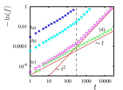
Figure 4: The fidelity decay for static imperfections [curves (a), (b), (c) with same values for $n_{q}$ and $\varepsilon$ as in Fig. 3] and random errors [curve (d) with $n_{q}=10$ and $\varepsilon=1.59\cdot 10^{-4}$] as a function of $t$ in a double logarithmic representation. The full lines correspond to power laws: $-\ln(f)\sim t$ and: $-\ln(f)\sim t^{2}$. The value of $\varepsilon$ for (d) is chosen such that the average reduction of fidelity for one elementary quantum gate is the same as for (c). The vertical dashed line provides the approximate position $0.5\sigma t_{\rm H}$ where the curves (a), (b), (c) change from linear to quadratic behavior.

We now consider the precise model of static imperfections given by Eq. (21). We have numerically calculated the fidelity $f(t)$ for the tent map with $K=1.7$ for $n_{q}\in\{6,\,8,\,10,\,12,\,14,\,16,\,18\}$ and $5\cdot 10^{-7}\leq\varepsilon\leq 10^{-4}$. For most cases we have determined the fidelity decay up to time scales $t\leq t_{max}$ with $f(t_{max})=0.5$ (except for $n_{q}=18$ and the smallest values of $\varepsilon$) since we are mostly interested in the regime $(1-f)\ll 1$ for which the analytical theory of the previous section is valid. We have also considered values $\varepsilon>10^{-4}$ but here the value $t_{max}$ is typically so small that the number of available data points is not useful for the scaling analysis given below. In most cases we have concentrated on one particular realization of the random coefficients $\delta_{i}$ and $J_{i}$. But we also have made checks with up to 200 particular realizations. As initial state $|\psi(t=0){>}$ we have chosen a coherent state $|\varphi(p_{0},\theta_{0}){>}$ [see next section, Eqs. (64), (65)] which is quite well localized around a classical point $(p_{0},\theta_{0})$ in phase space with a relative width $\sim 1/\sqrt{N}\sim 2^{-n_{q}/2}$ in both directions.

First, we chose a state close to the hyperbolic fix point $\theta=\pi/2$, $p=0$, well inside the chaotic region of phase space. As can be seen in Fig. 2 after $t=15$ iterations the state fills up a big fraction of the chaotic region and after $t\approx 30$ the state is practically ergodic. It covers then a fraction $\sigma\approx 0.65$ of phase space.

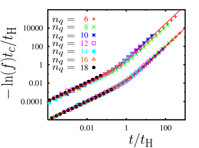
Figure 5: Scaling representation of the fidelity $f$ for one particular realization of static imperfections. The upper scaling curve shows: $-\ln(f)t_{c}/t_{\rm H}$ as a function of $t/t_{\rm H}$ with the two theoretical time scales $t_{c}=(\varepsilon^{2}n_{q}n_{g}^{2})^{-1}$ and $t_{\rm H}=2^{n_{q}}$. The full line in the upper curve corresponds to the theoretical random matrix result (44), (45) for $\beta=1$. The lower scaling curve (shifted down by a factor 0.01) correspond to $-\ln(f)\tilde{t}_{c}/\tilde{t}_{\rm H}$ versus $t/\tilde{t}_{\rm H}$ with the times scales $\tilde{t}_{c}$ and $\tilde{t}_{\rm H}$ obtained from the fit (59) (using appropriate weight-factors; see text) for each value of $n_{q}$ and $\varepsilon$. Here the full line corresponds to the analytical scaling curve: $y=x+x^{2}$ (with $y=-\ln(f)\tilde{t}_{c}/\tilde{t}_{\rm H}$ and $x=t/\tilde{t}_{\rm H}$). Data points are shown for $\varepsilon=5\cdot 10^{-7}$ (and $6\leq n_{q}\leq 18$); points for other values of $\varepsilon$ with $5\cdot 10^{-7}\leq\varepsilon\leq 10^{-4}$ fall on the same scaling curve and are not shown.

We have already seen in Fig. 3 of section 4 that the fidelity decay for static imperfections is faster than the exponential behavior for random errors. In order to analyze this in more detail we show in a double logarithmic representation in Fig. 4: $-\ln(f(t))$ as a function of $t$ for the three cases already shown in Fig. 3 ($n_{q}=10$ and $\varepsilon=3\cdot 10^{-5},\,6\cdot 10^{-6},\,5\cdot 10^{-7}$). For comparison, we also provide one case for random errors ($n_{q}=10$ and $\varepsilon=1.59\cdot 10^{-4}$).

For the static imperfections, we can clearly identify a transition from linear to quadratic behavior at a time scale $0.5\sigma t_{\rm H}\approx 0.325t_{\rm H}$ corresponding to the theoretical expression (54). However, the quadratic regime is best visible for the smallest values of $\varepsilon$ due to the restriction $-\ln(f)\leq\ln(2)$. For the case of random errors there is no such transition and the linear behavior applies for all time scales.

To analyze this transition in a quantitative way we determine for each value of $n_{q}$ and $\varepsilon$ two time scales $\tilde{t}_{c}$ and $\tilde{t}_{\rm H}$ by the numerical fit

$$y(t)=\frac{t}{\tilde{t}_{c}}+\frac{t^{2}}{\tilde{t}_{c}\tilde{t}_{\rm H}}\quad,\quad y(t)=-\ln(f(t))\ .$$ (59)

In order to prevent this fit to be artificially dominated by the large values of $t$ (i.e. the quadratic regime) we minimize:

$$d(a_{0},a_{1})=\sum_{t}w(t)\left[y(t)-a_{0}t-a_{1}t^{2}\right]^{2}$$ (60)

with an appropriate weight factor $w(t)\sim 1/(t\,y^{2}(t))$. The factor $1/y^{2}$ ensures that the vertical distance to be minimized is measured in the logarithmic representation for $y$. The other factor $1/t$ takes into account that the horizontal density of data points in the logarithmic representation increases with $t$. The fit procedure (60) corresponds therefore to a fit in log-log representation such that also the small time scales (and values of $y$) are taken properly into account.

According to the theoretical expression (54) one expects that:

$$\tilde{t}_{c}=t_{c}=\frac{1}{\varepsilon^{2}n_{q}n_{g}^{2}}\quad,\quad\tilde{t}_{\rm H}=0.5\,\sigma\,t_{\rm H}\approx 0.325\,t_{\rm H}$$ (61)

with $t_{\rm H}=2^{n_{q}}$ and $n_{g}=n_{q}^{2}-\frac{11}{2}n_{q}+4$. This theoretical prediction is verified in Figs. 5-8.

In Fig. 5, we show two types of scaling curves for the fidelity. The first (upper) curve shows: $-\ln(f)t_{c}/t_{\rm H}$ versus $t/t_{\rm H}$ with the time scales $t_{c}$ and $t_{\rm H}$ given above. We observe that the numerical data coincide very well for $n_{q}\geq 10$ with the analytical random matrix result (44),(45) for $\beta=1$. The data for $n_{q}=6,\,8$ show a moderate deviation for $t>t_{\rm H}$. We note that for this first scaling curve the dependence of the scaling parameters $t_{c}$ and $t_{\rm H}$ on $\varepsilon$ and $n_{q}$ is entirely determined by their theoretical expressions. This is different for the second (lower) scaling curve where: $-\ln(f)\tilde{t}_{c}/\tilde{t}_{\rm H}$ versus $t/\tilde{t}_{\rm H}$ is shown. Here the scaling parameters $\tilde{t}_{c}$ and $\tilde{t}_{\rm H}$ have been obtained by the fit (59) for each value of $n_{q}$ and $\varepsilon$. Therefore all data coincide well with analytical scaling expression (59).

It is important to note that both scaling curves cover 10 orders of magnitude and provide a strong confirmation of the crossover from linear to quadratic behavior predicted by the RMT approach. We mention as a side remark that we have also performed a similar scaling analysis for the case of random errors. Here the scaling curve is purely linear in accordance with Fig. 3. However, this gives a stronger confirmation of the linear behavior than in Fig. 3 since there the data for small $\varepsilon$ and large $n_{q}$ corresponding to the regime $(1-f)\ll 1$ are quite badly visible in contrast to the scaling curve.

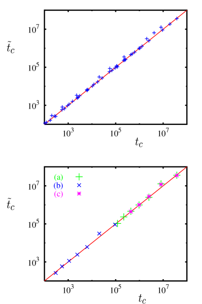
Figure 6: The time scale $\tilde{t}_{c}$ obtained from the fit: $-\ln(f)=t/\tilde{t}_{c}+t^{2}/(\tilde{t}_{c}\tilde{t}_{\rm H})$ versus the theoretical expression $t_{c}=(\varepsilon^{2}n_{q}n_{g}^{2})^{-1}$ in a double logarithmic representation. The full line corresponds to $\tilde{t}_{c}=t_{c}$. The data points of top panel correspond to the same realization of static imperfections as in Fig. 5 with $6\leq n_{q}\leq 18$ and $5\cdot 10^{-7}\leq\varepsilon\leq 10^{-4}$. The bottom panel shows again the data points for $6\leq n_{q}\leq 18$ and $\varepsilon=5\cdot 10^{-7}$ (a) and $\varepsilon=10^{-5}$ (b) for the same realization. The data points (c) are obtained from $\langle\tilde{t}_{c}^{-1}\rangle^{-1}$ where $\langle\cdots\rangle$ denotes the average over 200 realizations of static imperfections for each value of $n_{q}=6,\,8,\,10,\,12,\,14$ and $\varepsilon=5\cdot 10^{-7}$ (statistical error bars are smaller than symbol size).

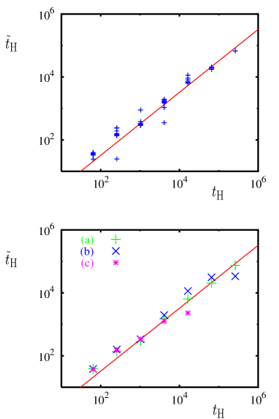
Figure 7: The time scale $\tilde{t}_{\rm H}$ obtained from the fit: $-\ln(f)=t/\tilde{t}_{c}+t^{2}/(\tilde{t}_{c}\tilde{t}_{\rm H})$ versus the Heisenberg time $t_{\rm H}=2^{n_{q}}$ in a double logarithmic representation. The full line corresponds to $\tilde{t}_{\rm H}=0.5\sigma t_{\rm H}$. The data points in the top panel correspond to the same realization of static imperfections as in Fig. 5 with $6\leq n_{q}\leq 18$ and $5\cdot 10^{-7}\leq\varepsilon\leq 10^{-4}$. The bottom panel shows again the data points for $6\leq n_{q}\leq 18$ and $\varepsilon=5\cdot 10^{-7}$ [data points (a)] and $\varepsilon=10^{-5}$ [data points (b)] for the same realization. The data points (c) are obtained from $\langle\tilde{t}_{c}^{-1}\rangle\langle(\tilde{t}_{c}\tilde{t}_{\rm H})^{-1}\rangle^{-1}$ where $\langle\cdots\rangle$ denotes the average over 200 realizations of static imperfections for each value of $n_{q}=6,\,8,\,10,\,12,\,14$ and $\varepsilon=5\cdot 10^{-7}$ (statistical error bars are smaller than symbol size).

In Figs. 6 and 7, the time scales $\tilde{t}_{c}$ and $\tilde{t}_{\rm H}$ obtained from the fit (59) are shown versus $t_{c}$ and $t_{\rm H}$. We observe that the first theoretical expectation $\tilde{t}_{c}=t_{c}$ is very well verified for the majority of data points. The small deviation for the remaining points appear for small $n_{q}$ and the largest values of $\varepsilon$ where the fit procedure is less reliable. The second identity $\tilde{t}_{\rm H}=0.325\,t_{\rm H}$ is in general also quite well verified. However, the deviations are slightly larger especially for larger values of $\varepsilon$. Furthermore, for $n_{q}>14$ the regime $t\gg t_{\rm H}$ is numerically not accessible and the fit procedure amounts to extrapolate $\tilde{t}_{\rm H}$ from data points $t\sim t_{\rm H}$ or even $t<t_{\rm H}$ for $n_{q}=16,\,18$.

We also note that the data points for $n_{q}=6,\,8$ (lower panel of Fig. 7) lie above the theoretical line in accordance with the first scaling curve in Fig. 5.

We have also determined the time scale $t_{f}$ at which $f(t_{f})=0.9$. The theoretical expression (54) suggests :

$$t_{f}=\frac{2t_{c}\,\ln(\frac{10}{9})}{1+\sqrt{1+\frac{8}{\sigma}\,\frac{t_{c}}{t_{\rm H}}\,\ln(\frac{10}{9})}}\approx\frac{0.2107\cdot t_{c}}{1+\sqrt{1+1.2967\,\frac{t_{c}}{t_{\rm H}}}}\ .$$ (62)

For $t_{c}\ll t_{\rm H}$ this implies $t_{f}\approx t_{c}\,\ln(\frac{10}{9})$ while for $t_{c}\gg t_{\rm H}$ we have $t_{f}\sim\sqrt{t_{c}\,t_{\rm H}}=\sqrt{t_{c}}\,2^{n_{q}/2}$. In Fig. 8, we show $t_{f}$ obtained from the numerical data for $\varepsilon=10^{-5},\ 5\cdot 10^{-7}$ and all values of $n_{q}$. The data points for $n_{q}\geq 10$ coincide very well with (62) while the points for $n_{q}=6,\,8$ lie slightly above the theoretical line. For comparison, we also show the time scale $t_{f}$ obtained from the simplified exponential behavior $f(t)=\exp(-t/t_{c})$. Generally, $t_{f}$ is believed to decrease with increasing $n_{q}$ and fixed $\varepsilon$. However, this is not the case if $t_{c}>t_{\rm H}$, i.e. for $\varepsilon<2^{-n_{q}/2}/(n_{g}\sqrt{n_{q}})$. For very small values of $\varepsilon$ there is certain regime where $t_{f}$ first slightly increases with $n_{q}$ and then decreases.

In all presented numerical studies we considered the static couplings between qubits ordered on a line. To check that the results are not sensitive to this specific configuration we also considered the case when qubits are located on a square lattice as it was discussed in georgeot . The obtained results (that we do not show here) confirms the RMT scaling (54).

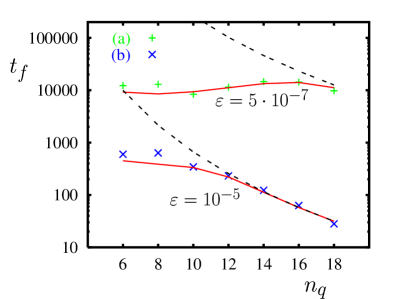
Figure 8: The time scale $t_{f}$ determined by $f(t_{f})=0.9$ (in a logarithmic representation) as a function of the number of qubits $n_{q}$. The data points correspond to the numerical simulation for the same realization of static imperfections as in Fig. 5 with $\varepsilon=5\cdot 10^{-7}$ (a) and $\varepsilon=10^{-5}$ (b). The two full lines correspond to $t_{f}$ given by (62) assuming the theoretical expression Eq. (54) for the fidelity. The two dashed curves correspond to $t_{f}=t_{c}\,\ln(\frac{10}{9})$ for the simplified exponential behavior $f(t)=\exp(-t/t_{c})$.

The case of the quantum evolution inside the integrable component of the tent map is analyzed in Figs. 9-11. Here, the initial state is located at $\theta=5.35$ and $p=0$ which is in middle between the center fix point ($\theta=3\pi/2$, $p=0$) and the boundary of the stable island ($\theta\approx 6.0$, $p=0$). We have determined for this case the time scales $\tilde{t}_{c}$ and $\tilde{t}_{\rm H}$ from the fit (59) and performed the same scaling analysis in Fig. 9 for the fidelity decay as in in Fig. 5 for the initial condition in the chaotic component. The scaling curves with the theoretical expressions (61) for $t_{c}$ and $t_{\rm H}$ give a significant deviation from the RMT result (upper group of curves in Fig. 9). To understand the reason of this dispersion we also show the scaling curves with the fitted time scales $\tilde{t}_{c}$ and $\tilde{t}_{\rm H}$. This procedure gives a good scaling of numerical data (lower group of curves in Fig. 9). Obviously, the fit (59) still works quite well as such but the obtained fit parameters are eventually different from the initial condition in the chaotic component and the RMT.

The dependence of $\tilde{t}_{c}$ on the theoretical value of $t_{c}$ is presented in Fig. 10. It shows that the theoretical expression works with a good accuracy in the interval of 6 orders of magnitude. This is not really a surprise since according to (26) $t_{c}^{-1}$ measures the overall strength of the perturbation. However, for $\tilde{t}_{\rm H}$ shown in Fig. 11 the situation is much more complicated. The variation of $\tilde{t}_{\rm H}$ vs. $t_{\rm H}=2^{n_{q}}$ shows unusual steps and it is unclear what is the real dependence in the limit of large $n_{q}$. Further studies are required for complete understanding of the static imperfection effects in this regime. This fact compromises the possibility to determine the asymptotic dependence of $t_{f}$ on $\varepsilon$ and $n_{q}$ for the case of integrable or quasi-integrable dynamics. In addition, the data of Fig. 8 show that it is not easy to determine the asymptotic behavior of $t_{f}$ in absence of clear scaling laws. Due to these two remarks we think that the scaling dependence for $t_{f}$ time scale, proposed in benentist ; wavelet for the case of static imperfections, represents in fact only an intermediate behavior and cannot be extrapolated to the limit of large $n_{q}$. Indeed, the quantum evolutions studied in benentist ; wavelet correspond to quasi-integrable regimes and additional tests are required to check the validity of the RMT scaling (54) for the quantum algorithms studied there.

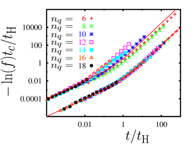
Figure 9: Scaling curve for fidelity as in the case of Fig. 5 but for the quantum evolution inside integrable component. Here, the initial state is a minimal coherent wave packet taken inside the regular part of phase space at $\theta=5.35$ and $p=0$; the same realization of static imperfections as in Fig. 5 is used.

Finally, it is interesting to compare directly the fidelity decay induced by static imperfections for the quantum evolution in chaotic and integrable components (see Fig.12). The numerical data show that $f(t)$ decreases faster in the case of integrable evolution. As it was discussed in prosen the presence of chaos reduces the fidelity decay rate. This is in the agreement with the results of Fig. 7 and Fig. 11 according to which $\tilde{t}_{\rm H}$ is much smaller for the integrable regime as for the regime of quantum chaos. However, the possibility of using this fact to improve the accuracy of quantum computations remains an open question.

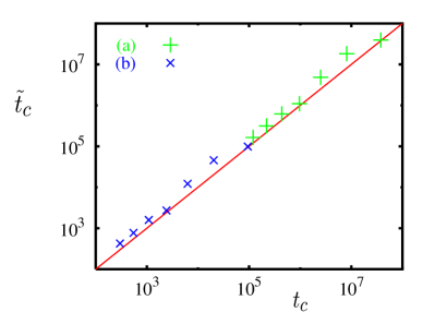
Figure 10: The time scale $\tilde{t}_{c}$ as in Fig. 6 versus $t_{c}=(\varepsilon^{2}n_{q}n_{g}^{2})^{-1}$, data are obtained from Fig. 9 for the case of regular dynamics. Shown are data points for $\varepsilon=5\cdot 10^{-7}$ (a) and $\varepsilon=10^{-5}$ (b) with $6\leq n_{q}\leq 18$ in a double logarithmic representation. The full line corresponds to $\tilde{t}_{c}=t_{c}$.

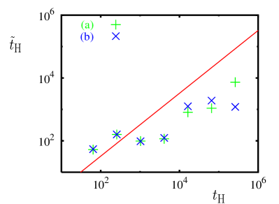
Figure 11: The time scale $\tilde{t}_{\rm H}$ as in Fig. 7 versus $t_{\rm H}=2^{n_{q}}$, data are obtained from Fig. 9 for the case of regular dynamics. Shown are data points for $\varepsilon=5\cdot 10^{-7}$ (a) and $\varepsilon=10^{-5}$ (b) with $6\leq n_{q}\leq 18$ in a double logarithmic representation. The full line corresponds to $\tilde{t}_{\rm H}=0.5\sigma t_{\rm H}$.

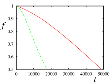
Figure 12: fidelity decay for initial minimal coherent state in chaotic (full curve) and integrable (dashed curve) component for $n_{q}=16$, $\varepsilon=5\cdot 10^{-7}$.

The numerical data presented in this section definitely confirm the RMT universal law for fidelity decay for the case when the evolution takes place in the regime of quantum chaos. This means that this law works for quantum algorithms simulating a complex dynamics. The situation for the evolution in the integrable component is more complicated. The data show that the theoretical expression for $t_{c}$ is still valid but the dependence of the time scale $\tilde{t}_{\rm H}$ on $n_{q}$ requires further investigations.

It is interesting to note that the relation (54) should also work for the problem of Loschmidt echo in systems with quantum chaos pastawski ; beenakker ; como ; prosen ; cohen . In this case for small perturbations $t_{c}$ is still given by Eq. (26) or, that is equivalent, the inverse decrease rate is given by the Fermi golden rule beenakker . Then the scale $t_{\rm H}$ is determined by the inverse density of states or for quantum maps by the number of states via relation $t_{\rm H}=N$. As a result for small perturbations the decay of Loschmidt echo for such quantum dynamics is still given by the universal decay relation Eq. (54).

7 Husimi function

Here we discuss how an arbitrary quantum state $|\psi{>}$ can be represented in the classical phase space in the process of quantum computation. For this it is convenient to use the coarse-grained Wigner function (or the Husimi function) wigner ; husimi :

$$\rho_{H}(p_{0},\theta_{0})=|{<}\varphi(p_{0},\theta_{0})\,|\,\psi{>}|^{2}$$ (63)

where the smoothing is done with the coherent state

$$|\varphi(p_{0},\theta_{0}){>}=A\sum_{p}e^{-(p-p_{0})^{2}/4a^{2}-i\theta_{0}p}\,|p{>}\ .$$ (64)

Here, $A$ is the normalization constant and $a$ is the width of the coherent state in the $p$-representation. The coherent state corresponds to a gaussian wave packet that is localized in the classical phase space around a point $(\theta_{0},\,p_{0})$ with widths $\Delta p=a$ and $\Delta\theta=1/(2a)$. We choose $a=\sqrt{N/12}$ such that the widths relative to the size of the phase space are comparable:

$$\frac{\Delta p}{N}=\frac{1}{\sqrt{12N}}\approx\frac{0.2887}{\sqrt{N}}\quad,\quad\frac{\Delta\theta}{2\pi}=\frac{\sqrt{3}}{2\pi\sqrt{N}}\approx\frac{0.2757}{\sqrt{N}}\ .$$ (65)

The naive evaluation of the Husimi function (63) without any optimization requires ${\cal O}(NN_{p}N_{\theta})$ operations (on a classical computer) where $N_{p}$ and $N_{\theta}$ are the numbers of values for $p_{0}$ and $\theta_{0}$ for which (63) is evaluated. In view of Eq. (65) it is sufficient to choose $N_{p}=N_{\theta}=\sqrt{N}$ resulting in ${\cal O}(N^{2})$ operations which is very expensive as compared to ${\cal O}(N\log(N)^{2})$ operations needed by the simulation of the quantum map on a classical computer as described in Sec. 3.

Fortunately, the evaluation of the Husimi function can be done in a more efficient way. To motivate and explain this let us first consider a modified Husimi function defined by:

$$\rho_{H}^{(p)}(p_{0},\theta_{0})=|{<}\varphi^{(p)}(p_{0},\theta_{0})\,|\,\psi{>}|^{2}$$ (66)

with the modified coherent state:

$$|\varphi^{(p)}(p_{0},\theta_{0}){>}=\frac{1}{\sqrt[4]{N}}\sum_{p=p_{0}}^{p_{0}+\sqrt{N}-1}e^{-i\theta_{0}p}\,|p{>}\ .$$ (67)

Here we assume for the sake of simplicity that the number of qubits $n_{q}$ is even such that $\sqrt{N}=2^{n_{q}/2}$ is integer. We furthermore require that $p_{0}$ is an integer multiple of $\sqrt{N}$ and $\theta_{0}=2\pi\,l/\sqrt{N}$ with $l=0,\,\ldots,\,\sqrt{N}-1$.

Comparing (64) with (67), we see that the gaussian pre-factor has been replaced by a box-function of width $\sqrt{N}$. This provides a very good localization for the momentum representation but implies that in angle representation the amplitude around $\theta_{0}$ decreases only as a power law according to the Fourier transform of the box-function: $\sin(x)/x$ with $x=\sqrt{N}(\theta-\theta_{0})/2$. However, the modified coherent state (67) still provides a quite well localized state around the point $(\theta_{0},\,p_{0})$. Its main advantage is related to the fact that it can be put in the form:

$$|\varphi^{(p)}(p_{0},\theta_{0}){>}=\tilde{U}_{\rm QFT}^{-1}\,|p_{0}+l{>}$$ (68)

where $\theta_{0}=2\pi\,l/\sqrt{N}$ and $\tilde{U}_{\rm QFT}$ corresponds to the quantum Fourier transform operator (see (13)) for the first half of the qubits ($\alpha_{0},\,\ldots,\,\alpha_{n_{q}/2-1}$). Eq. (68) implies that

$$\rho_{H}^{(p)}(p_{0},\theta_{0})=|{<}p\,|\,\tilde{U}_{\rm QFT}\,|\,\psi{>}|^{2}$$ (69)

with $p=p_{0}+l=p_{0}+\sqrt{N}\theta_{0}/(2\pi)$. Here the state $\tilde{U}_{\rm QFT}\,|\,\psi{>}$ can be evaluated efficiently on a quantum computer using $\frac{n_{q}}{4}(\frac{n_{q}}{2}+1)$ elementary quantum gates according to (19) (with $n_{q}$ replaced by $n_{q}/2$). Emulating the quantum computer on a classical computer this still costs only ${\cal O}(N\log(N)^{2})$ elementary operations. The matrix elements ${<}p|\,\tilde{U}_{\rm QFT}\,|\,\psi{>}$ of this state with the momentum eigenstates $|p{>}$ provide directly via Eq. (69) the modified Husimi function. Here the value of $p=0,\,\ldots\,N-1$ contains in its first half of the binary digits the information for $\theta_{0}$ and in its second half the information for $p_{0}$. More explicitly, if $p=\sum_{j=0}^{n_{q}-1}\alpha_{j}2^{j}$, we have :

$$p_{0}=\sum_{j=n_{q}/2}^{n_{q}-1}\alpha_{j}2^{j}\quad,\quad\theta_{0}=\frac{2\pi}{\sqrt{N}}\sum_{j=0}^{n_{q}/2-1}\alpha_{j}2^{j}\ .$$ (70)

We note that it is also possible to introduce another type of modified Husimi function (and modified coherent state) by exchanging the roles of $\theta_{0}$ and $p_{0}$ :

$$\rho_{H}^{(\theta)}(p_{0},\theta_{0})=|{<}p\,|\,\tilde{U}_{\rm QFT}^{-1}\,U_{\rm QFT}\,|\,\psi{>}|^{2}\ .$$ (71)

where $p=N\theta_{0}/(2\pi)+p_{0}/\sqrt{N}$. As in Eq. (67), we require that $p_{0}$ is an integer multiple of $\sqrt{N}$ and $\theta_{0}=2\pi\,l/\sqrt{N}$ with $l=0,\,\ldots,\,\sqrt{N}-1$. The operator $U_{\rm QFT}$ corresponds to quantum Fourier transform for all qubits and transforms a state from $p$- to $\theta$-representation. $\tilde{U}_{\rm QFT}$ corresponds as above to quantum Fourier transform for the first half of the qubits. We mention that the coherent states associated to (71) have a power-law localization amplitude for $p$ and a box-function localization amplitude for $\theta$.

We have seen that both types of modified Husimi       functions can be evaluated on a classical computer with ${\cal O}(N\log(N)^{2})$ operations. Based on the idea of the QFT which is closely related to the FFT if simulated on a classical computer, we have also implemented an efficient classical algorithm for the original Husimi function (63) with the gaussian coherent states. For each value of $p_{0}$, we only consider the restricted sum such that $|p-p_{0}|\leq 4\sqrt{N}$ and evaluate the matrix elements ${<}\varphi(p_{0},\theta_{0})\,|\,\psi{>}$ for all values of $\theta_{0}$ simultaneously using FFT. This provides also an algorithm with complexity ${\cal O}(N\log(N)^{2})$ but with a considerably larger numerical pre-factor. However, this method does not allow for a “pure” quantum computation as it is possible for the two types of modified Husimi functions.

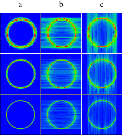
Figure 13: Density plots of the three different types of Husimi functions for the circle-state (72) with $n_{q}=10,\ 12,\ 14$ (rows from top to bottom). The horizontal axis corresponds to $\theta_{0}\in[0,2\pi[$ and the vertical axis to $p_{0}\in[0,N[$. The density is minimal for blue/black and maximal for red/white. Column (a) corresponds to the Husimi function (63) with gaussian amplitude, column (b) to the momentum modified Husimi function (66) and column (c) to the phase modified Husimi function (71).

In order to compare the different Husimi functions, we consider a test-state defined by a circular superposition of coherent states as:

$$|\psi_{\rm circle}{>}=\tilde{A}\sum_{(p_{0},\theta_{0})\in\bigcirc}|\varphi(p_{0},\theta_{0}){>}\ .$$ (72)

Here $\tilde{A}$ is a normalization constant and the sum runs over a discrete set of points $(\theta_{0},p_{0})$ on a circle with center $(\pi,N/2)$ and relative diameter 0.7 (as compared to the size of the phase space).

In Fig. 13, we show the density plots for the three types of Husimi functions for this test-state with $n_{q}=10,\ 12,\ 14$. In all cases the circle picture of the density is quite well reproduced and one clearly sees that the circle has a finite width according to the widths of the coherent states due to the quantum uncertainty principle (see Eq. (65)). For the modified Husimi function (66) (column (b)), one clearly observes the effect of the power-law decrease for the $\theta$-amplitude leading to a smearing out of maxima in the $\theta$-direction. The same holds for the second modified Husimi function (71) (column (c)) concerning the $p$-direction. This effect is strongest for small values of $n_{q}$ and becomes smaller with increasing $n_{q}$. The effect of smearing out is not visible for the original Husimi function (63) (column (a)) with gaussian amplitudes for $\theta$ and $p$.

In order, to study the evolution of the Husimi function for chaotic and regular regimes in the quantum tent map, we choose as initial condition the circle-state (72). The semi-classical density of this state intersects quite well with both regular and chaotic parts of the mixed phase space (see Figs. 1,2).

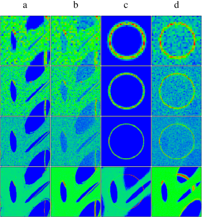
Figure 14: Density plot of the Husimi function (63) from the the circle-state (72) after 100 iterations with the quantum map with $K=kT=1.7$ and $T=2\pi/N=2\pi/2^{n_{q}}$ (columns (a) and (b)) and after 100 iterations in the future and 100 iterations with the inverse map in the past (columns (c) and (d)). The first three rows correspond to $n_{q}=10,\ 12,\ 14$ (from top to bottom) and the last row corresponds a classical density plot obtained from a histogram-sampling with a box-size corresponding to the resolution for $n_{q}=14$ and with an average number of 100 classical trajectories per box. Columns (a) and (c) correspond to the exact quantum or classical maps only limited by the relative machine precision $10^{-16}$. Columns (b) and (d) correspond to the quantum computation with random errors in quantum gates ($\varepsilon=0.01$) or perturbed the classical map perturbed by noise with $\varepsilon=0.01$ (see text).

In Fig. 14 we show the density-plots of the Husimi functions (defined by Eq. (63) of the state obtained from the circle-state after 100 iterations of the quantum map for the cases $n_{q}=10,\ 12,\ 14$ (column (a)). We also show the state that is obtained by applying further 100 iterations of the inverse quantum map which should theoretically provide the original circle-state (column (c)). In Fig. 14 we also show a density-plot for the classical map (3) (with $p$ to be taken modulo $2\pi/T$). Here we have determined the classical trajectories of $100N$ random initial points on the circle. Then the density-plot has been calculated from a histogram with a finite box-size corresponding to the finite resolution of the quantum case with $n_{q}=14$.

One clearly sees in column (a) that the chaotic part of the phase space is filled up ergodically while the piece of the circle intersecting the regular part of the phase space remains a connected line. Actually, this line rotates with a constant angular velocity around the center fix-point due to the local linear behavior of $V^{\prime}(\theta)$ close to the fix-point.

Concerning the states obtained after the back-iteration in time, which are shown in column (c), one observes that the inverse quantum map reproduces exactly the initial state while for the classical map only the pieces of the circle belonging to the regular part of the phase space are reproduced. This is due to the finite machine precision (of $10^{-16}$) together with the exponential instability in the chaotic part of the phase space. We have verified that for only 25 iterations, the circle is well reproduced in every part of the phase space. At 50 iterations the classical computer round-off errors already have significant effects but are not sufficient to create a uniform distribution in the chaotic region as it is the case with 100 iterations shown in Fig. 14, last row of column (c). This effect is completely absent in the quantum simulation. The information for the phase space distribution is encoded in the quantum state in such a way that it is not sensible to the round-off errors of the classical computer simulating the quantum algorithm for the tent map.

To investigate this point in more detail, we have also performed a quantum simulation where all quantum gates are perturbed by random errors (see Sec. 3). The effects of this noisy perturbation can be seen in Fig. 14 in the columns (b) (100 forward iterations of the circle-state) and (d) (100 forward and 100 backward iterations) where we have chosen $\varepsilon=0.01$. Concerning the quantum map, the noise reduces some-how the general quality of the pictures but it does not distinguish between chaotic and regular regions of the phase space. In particular in column (d), the circular density is quite well reproduced with some additional overall noise. Concerning the classical map, the circle-pieces in the regular region still remain closed lines but they acquire a finite width which increases in a diffusive way with the number of iterations. The circle-pieces in the chaotic region become very quickly mixed. Furthermore, it is not possible to reproduce the initial circle in the chaotic region due to the exponential instability (last row of column (d)). We have verified that this effect is already true for only 15 forward and 15 backward iterations if $\varepsilon=0.01$ (for the classical map the noise is introduced in the equation for momentum with an amplitude $\varepsilon=0.01$, Fig. 14 bottom d).

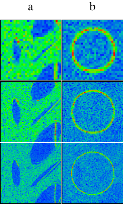
Figure 15: Density plot of the Husimi function (63) from the the circle-state (72) after 100 iterations with the quantum map (same values as in Fig. 14) perturbed by static errors (see text) with $\varepsilon=10^{-5}$ (column (a)) and after 100 iterations in the future and 100 iterations with the inverse perturbed map in the past (column (b)). The different rows correspond to $n_{q}=10,\ 12,\ 14$ (from top to bottom).

We have also studied the effects of static imperfections on the Husimi function evolution in the tent map. In Fig. 15, we show the results of static imperfections with $\varepsilon=10^{-5}$ and $n_{q}=10,\ 12,\ 14$. The initial state is again the circle-state and column (a) corresponds to the state after 100 forward iterations and column (b) to the state after 100 forward and 100 backward iterations. The effect is quite similar to the quantum computation with random errors (columns (b) and (d) of Fig. 14). The general quality of the pictures is reduced and there is no distinction between regular and chaotic part of the phase space. Again, in column (b) the circular density is quite well reproduced with some additional overall noise. We should note that the static imperfections of strength $\varepsilon=10^{-5}$ give perturbations in the Husimi function which are comparable with those in the case of random errors at $\varepsilon=0.01$. This shows that the static imperfections perturb the quantum computations in a stronger way comparing to random errors.

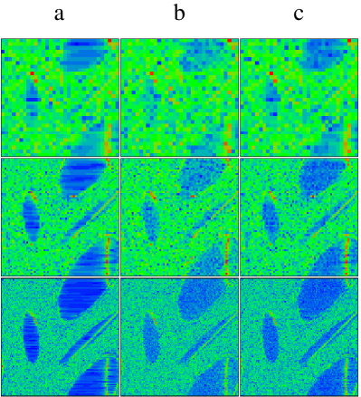
Figure 16: Density plot of the modified Husimi function (66) from the the circle-state (72) after 100 iterations with the quantum map (same values as in Fig. 3). Column (a) corresponds to the exact quantum map, column (b) to the map with random errors in quantum gates with $\varepsilon=0.01$ and column (c) to the quantum map simulated with static imperfections with $\varepsilon=10^{-5}$. The different rows correspond to $n_{q}=10,\ 12,\ 14$ (from top to bottom).

Finally, we show in Fig. 16 the modified Husimi functions (66) after 100 iterations applied to the initial circle-state again for the three cases $n_{q}=10,\ 12,\ 14$. Column (a) shows the exact simulation, (b) the case of random errors ($\varepsilon=0.01$) and (c) the quantum map with static imperfections ($\varepsilon=10^{-5}$). We note that the smearing-out effect discussed at the beginning of this Section (see Fig. 13) is well visible for the case of the exact simulation, while it is not visible at all for the cases with random errors or static imperfections. Therefore, the utilization of the modified Husimi function seems to be quite well justified in these cases.

8 Conclusion

The results obtained in this paper give a universal description of fidelity decay in quantum algorithms simulating complex dynamics on a realistic quantum computer with static imperfections. This decay is given by Eq. 54 which determines the time scale $t_{f}$ of reliable quantum computation with fidelity $f>0.9$. According to Eq. 54

$$t_{f}\approx t_{c}/10=1/(10\varepsilon^{2}n_{q}n_{g}^{2})\;;\;N_{g}\approx 1/(10\varepsilon^{2}n_{q}n_{g})$$ (73)

for $t_{\rm H}>t_{c}$ so that $\varepsilon>\varepsilon_{ch}=2^{-n_{q}/2}/(n_{g}\sqrt{n_{q}})$. Here, $N_{g}=t_{f}n_{g}$ is the total number of gates which can be performed with fidelity $f>0.9$. In this regime the static errors act in a way similar to random noise errors even if their effect is stronger due to coherent accumulation of static errors inside a certain interval of the algorithm (one map iteration for the tent map). Indeed, for random errors in quantum gates the relation (4) gives

$$t_{f}\approx t_{r}/10\approx 5/(\varepsilon^{2}n_{g})\;;\;N_{g}\approx 5/\varepsilon^{2}.$$ (74)

We note that (74) is in agreement with the result obtained for random errors in a very different quantum algorithm wavelet and hence it is generic. Even if the dependence of $N_{g}$ on $\varepsilon$ in Eqs. (73), (74) is the same, the dependence on $n_{q}$ is rather different. This difference should play an important role for the quantum error correction codes which allow to perform the fault-tolerant quantum computation for the random error rate $p_{r}\sim\epsilon^{2}<10^{-4}$ (see e.g. steane ; chuang ; gottesman ; aharonov ; steane1 ). The fact that for random errors $N_{g}$ is independent of $n_{q}$ while for static imperfections $N_{g}$ drops strongly with $n_{q}$ should significantly decrease the threshold for fault-tolerant quantum computation in presence of static imperfections.

For $t_{c}<t_{\rm H}$ or $\varepsilon<\varepsilon_{ch}=2^{-n_{q}/2}/(n_{g}\sqrt{n_{q}})$ the time scale $t_{f}$ is given by the relation

$$t_{f}\approx 0.2\sqrt{t_{c}t_{\rm H}}\approx 2^{n_{q}/2}/(5\varepsilon n_{g}\sqrt{n_{q}})\;;\;N_{g}\approx 2^{n_{q}/2}/(5\varepsilon\sqrt{n_{q}}).$$ (75)

In this regime the effect of static imperfections is absolutely different from random noise errors. This regime may be dominant for up to 10 - 15 qubits. However, in the limit of large $n_{q}\gg 10$ it appears only in the limit of very small static imperfections and should not be very important for quantum computers with few tens of qubits. The transition from the regime (73) to regime (75) takes place for

$$\varepsilon>\varepsilon_{ch}=2^{-n_{q}/2}/(n_{g}\sqrt{n_{q}})\;.$$ (76)

From the physical point of view this border can be interpreted as the quantum chaos border above which the static imperfections start to mix the energy levels of ideal quantum algorithm. The fact that this border drops exponentially with the number of qubits $n_{q}$ has been discussed in benentiqcb for a quantum algorithm for complex dynamics. Above $\varepsilon_{ch}$ the effect of static imperfections becomes somewhat similar to random errors.

The results (73) and (75) for the time scales of reliable quantum computation are based on the RMT approach and are universal for algorithms which simulate a complex dynamics, e.g. an evolution in the regime of quantum chaos. However, it is important to keep in mind that there are other types of algorithms where the evolution is rather regular, e.g. the Grover algorithm or integrable dynamics. In such cases the asymptotic dependence of $t_{\rm H}$ on $n_{q}$ should be studied in more detail. It is not excluded that in such cases $t_{\rm H}$ grows with $n_{q}$ very slowly (see Fig. 11) or even may be independent of $n_{q}$. In such situations the static imperfections will generate a very significant reduction of the time scale of reliable quantum computation. In a sense our RMT result (54) gives the weakest form of fidelity decay in a realistic quantum computer with $n_{q}$ qubits since the reduction of the chaotic component $\sigma$ accelerates this decay.

The universal regime for fidelity decay in quantum computations established in this paper can also find other applications. For example it can appear in the decay of spin echo in interacting spin systems.

This work was supported in part by the EC IST-FET project EDIQIP and the NSA and ARDA under ARO contract No. DAAD19-01-1-0553 and by the French goverment grant ACI Nanosciences-Nanotechnologies LOGIQUANT. We thank CalMiP at Toulouse and IDRIS at Orsay for access to their supercomputers.

Upon completion of this manuscript a recent preprint of T. Gorin, T. Prosen, and T. H. Seligman gorin came to our attention where the relation between fidelity decay and two-level form factor has been established for an abstract Hamiltonian model with continuous time evolution and a perturbation given by an invariant random matrix. However, in this work only the regime of a small perturbation strength $\lambda\ll 1$ $(\lambda\sim\sqrt{t_{H}/t_{c}})$ is studied which translates to $t_{\rm H}\ll t_{c}$ with the dominant gaussian decay.

References

- (1) A. Ekert and R. Josza, Rev. of Mod. Phys. 68, 733 (1996).
- (2) A. Steane, Rep. Prog. Phys. 61, 117 (1998).
- (3) M.A. Nielsen and I.L. Chuang Quantum Computation and Quantum Information, Cambridge Univ. Press, Cambridge (2000).
- (4) D. P. Di Vincenzo, Science 270, 255 (1995).
- (5) P.W. Shor, in Proc. 35th Annual Symposium on Foundation of Computer Science, Ed. S.Goldwasser (IEEE Computer Society, Los Alamitos, CA, 1994), p.124
- (6) L. K. Grover, Phys. Rev. Lett. 79, 325 (1997).
- (7) S. Lloyd, Science 273, 1073 (1996).
- (8) G. Ortiz, J.E. Gubernatis, E. Knill, and R.Laflamme, Phys. Rev. A 64, 22319 (2001).
- (9) B.V.Chirikov, F.M.Izrailev and D.L.Shepelyansky, Sov. Scient. Rev. C (Gordon & Bridge) 2, 209 (1981); Physica D 33, 77 (1988).
- (10) F.M.Izrailev, Phys. Rep. 196, 299 (1990).
- (11) R. Schack, Phys. Rev. A 57, 1634 (1998).
- (12) B. Georgeot, and D.L. Shepelyansky, Phys. Rev. Lett. 86, 2890 (2001).
- (13) G. Benenti, G. Casati, S. Montangero, and D.L. Shepelyansky, Phys. Rev. Lett. 87, 227901 (2001).
- (14) A.D. Chepelianskii and D.L. Shepelyansky, Phys. Rev. A 66, 054301 (2002).
- (15) A.A. Pomeransky and D.L. Shepelyansky, Phys. Rev. A (to appear), quant-ph/0306203.
- (16) B. Georgeot and D.L. Shepelyansky, Phys. Rev. Lett. 86, 5393 (2001); ibid. 88, 219802 (2002).
- (17) M. Terraneo, B. Georgeot and D.L. Shepelyansky, Eur. Phys. J. D 22, 127 (2003).
- (18) W.H. Zurek, Rev. Mod. Phys. 75, 715 (2003).
- (19) B.Georgeot and D.L.Shepelyansky, Phys. Rev. E 62, 3504 (2000); 62, 6366 (2000).
- (20) V.V. Flambaum, Aust. J. Phys. 53, 489 (2000).
- (21) G. P. Berman, F. Borgonovi, F. M. Izrailev, and V. I. Tsifrinovich, Phys. Rev. E 64, 056226 (2001).
- (22) G. Benenti, G. Casati and D.L. Shepelyansky, Eur. Phys. J. D 17, 265 (2001).
- (23) D. Braun, Phys. Rev. A 65, 042317 (2002).
- (24) A. Peres, Phys. Rev. A 30, 1610 (1984).
- (25) D.L. Shepelyansky, Physica D 8, 208 (1983).
- (26) G. Casati, B.V. Chirikov, I. Guarneri and D.L. Shepelyansky, Phys. Rev. Lett. 56, 2437 (1986).
- (27) R.A. Jalabert and H.M. Pastawski, Phys. Rev. Lett. 86, 2490 (2001).
- (28) P.Jacquod, P.G.Silvestrov and C.W.J. Beenakker, Phys. Rev. E 64, 055203 (2001).
- (29) G. Veble and T. Prosen, Phys. Rev. Lett. 92, 034101 (2004).
- (30) G. Benenti and G. Casati, Phys. Rev. E 66, 066205 (2002).
- (31) T. Prosen and M. Znidaric, J. Phys. A 34, L681 (2001); J. Phys. A 35, 1455 (2002); T. Prosen, T.H. Seligman and M. Znidaric, Prog. Theor. Phys. Supp. 150, 200 (2003).
- (32) T. Kottos and D.Cohen, Europhys. Lett. 61, 431 (2003).
- (33) N.R. Cerruti and S. Tomsovic, Phys. Rev. Lett. 88, 054103 (2002); J. Phys. A 36, 3451 (2003).
- (34) Y. Adamov, I.V. Gornyi and A.D. Mirlin, Phys. Rev. E 67, 056217 (2003).
- (35) C. Miguel, J.P. Paz and W.H. Zurek, Phys. Rev. Lett. 78, 3971 (1997).
- (36) M. Terraneo and D.L. Shepelyansky, Phys. Rev. Lett. 90, 257902 (2003).
- (37) S. Bettelli, quant-ph/0310152.
- (38) F. J. Dyson, J. Math. Phys. 3, 140 (1962).
- (39) M.L. Mehta, Random Matrices (Academic, New York, 1991).
- (40) T. Guhr, A. Mueller-Groeling and H.A. Weidenmueller, Phys. Rep. 299, 189 (1998).
- (41) E. Wigner, Phys. Rev. 40, 749 (1932).
- (42) S.-J. Chang and K.-J. Shi, Phys. Rev. A 34, 7 (1986).
- (43) L.M.K.Vandersypen, M. Steffen, G. Breyta, C.S. Yannoni, M.H. Sherwood, and I.L. Chuang, Nature 414, 883 (2001).
- (44) Y.S. Weinstein, S. Lloyd, J. Emerson, and D.G. Cory, Phys. Rev. Lett. 89, 157902 (2002).
- (45) J. Emerson, Y.S. Weinstein, S. Lloyd and D.G. Cory, Phys. Rev. Lett. 89, 284102 (2002).
- (46) B.V. Chirikov, Phys. Rep. 52, 263 (1979).
- (47) S. Bullett, Com. Math. Phys. 107, 241 (1986).
- (48) V.V. Vecheslavov, Zh. Eksp. Teor. Fiz. 119, 853 (2001) (nlin.CD/0005048); V.V. Vecheslavov and B.V. Chirikov, Zh. Eksp. Teor. Fiz. 120, 740 (2001) (nlin.CD/0202017).
- (49) B.A. Muzykantskii and D.E. Khmelnitskii, Phys. Rev. B 51, 5481 (1995).
- (50) A.D. Mirlin, Phys. Rep. 326, 259 (2000).
- (51) G. Casati, G. Maspero and D.L. Shepelyansky, Phys. Rev. E 56, R6233 (1997).
- (52) D.V. Savin and V.V. Sokolov, Phys. Rev. E 56, R4911 (1997).
- (53) K.M. Frahm, Phys. Rev. E 56, R6237 (1997).
- (54) D. Gottesman, Phys. Rev. A 57, 127 (1998).
- (55) D. Aharonov and M. Ben-Or, quant-ph/9906129.
- (56) A. Steane, quant-ph/0207119.
- (57) G. Benenti, G. Casati, S. Montangero and D.L. Shepelyansky, Eur. Phys. J. D 20, 293 (2002).
- (58) B. L. Altshuler and B. I. Shklovskii, Zh. Eksp. Teor. Fiz. 91, 220 (1986) [Sov. Phys. JETP 64, 127 (1986)].
- (59) T. Gorin, T. Prosen, and T. H. Seligman, preprint nlin. CD/0311022v1.