Packet narrowing and quantum entanglement in photoionization and photodissociation

Abstract

The narrowing of electron and ion wave packets in the process of photoionization is investigated, with the electron-ion recoil fully taken into account. Packet localization of this type is directly related to entanglement in the joint quantum state of electron and ion, and to Einstein-Podolsky-Rosen localization. Experimental observation of such packet-narrowing effects is suggested via coincidence registration by two detectors, with a fixed position of one and varying position of the other. A similar effect, typically with an enhanced degree of entanglement, is shown to occur in the case of photodissociation of molecules.

I Introduction

In the course of photoionization, a photoelectron is ejected and the ion recoils, being constrained both by the conservation of momentum and energy and by the condition of the original atom. In principle this initial condition includes all aspects of the atom’s internal and center of mass states, but here we will focus for greatest clarity on an atom in its ground electronic state with a center of mass wave packet determined by whatever localizes the atom in the region of the photoionization. Although photoionization has been treated repeatedly in weak and strong fields (see, for example, Refs. Gottfried and MVF ), the focus has been mainly on cross sections and the dynamics of the particles, and there has been little discussion of the nature of the joint quantum state of the breakup fragments. This quantum state is entangled and it is closely related to questions of fundamental interest because the fragmentation process is exactly the one used by Einstein, Podolsky and Rosen (EPR) EPR to illustrate Einstein’s position regarding limitations of quantum theory. We identify the amount of state entanglement by examining the relative localization of the wavepackets of the electron and ion, under the simplifying assumptions that the incident photon momentum and the post-breakup Coulomb interaction can be neglected. The different time regimes for entanglement are identified.

Due to the finite mass of the particles, the wave function of the system changes drastically between the initial stage and the long-time limit. We find suitable measures of the entanglement of the electron and ion that are connected with their packet widths in position space, specifically the coincidence width and the single-particle width. In view of other treatments of breakup JHE2 , these localization measures give an alternative view of entanglement and reveal new channels for achieving high degrees of entanglement. Our choice of measure also identifies entanglement “control parameters” for comparison with those that have been advanced in previous studies of both photon-atom JHE and photon-photon PDC wave functions, and through conditional localization it is related to formal photonic analogues Reid of the EPR discussion and bimolecular breakup as a route to matter wave entanglement OK . More importantly, these widths are experimentally measurable entities. Finally, we discuss similar issues for dissociation of a diatomic molecule and explain the most significant differences in the results.

II Photoionization

Let an atom, originally in its ground state, be photoionized by a light field

$$\vec{\mathcal{E}}(t)=\vec{\mathcal{E}}_{0}\,\sin(\omega t),$$ (1)

where $\hbar\omega>|E_{0}|$ and $E_{0}$ is the ground state energy. It should be noted that by using the dipole approximation and ignoring the term $\vec{k}\cdot\vec{r}$ in the argument in Eq. (1) we are ignoring all recoil effects due to absorption of the photon momentum $\hbar\vec{k}$. This approximation is quite reasonable because there is another much stronger mechanism giving rise to recoil. In the process of photoionization an atomic electron acquires an energy $\sim\hbar\omega$ and hence a momentum $\sim\sqrt{m\hbar\omega}$, and the ion gets the same momentum (with the opposite sign), and this momentum is much larger than $\hbar k=\hbar\omega/c$. This is in contrast to the problems of entanglement in spontaneous photon emission of excited atoms and Raman scattering JHE .

To describe such a process with atomic recoil and with an initial wave-packet distribution of the atomic center of mass, let us begin from the Schrödinger equation for two particles - electron and ion - in the field. Traditionally, to separate variables in such an equation, we use the relative (rel) and center-of-mass (cm) position and momentum vectors LL

$$\begin{array}[]{ll}\vec{r}_{\text{rel}}=\vec{r}_{e}-\vec{r}_{i},&\vec{r}_{\text{cm}}=\displaystyle\frac{m_{e}\vec{r}_{e}+m_{i}\vec{r}_{i}}{M},\\ \vec{p}_{\text{rel}}=\displaystyle\frac{m_{i}\vec{p}_{e}-m_{e}\vec{p}_{i}}{M},&\vec{p}_{\text{cm}}=\vec{p}_{e}+\vec{p}_{i},\end{array}$$ (2)

where $\vec{r}_{e}$ and $\vec{r}_{i}$ are the electron and ion position vectors, $\vec{p}_{e}=-i\hbar\partial/\partial\vec{r}_{e}$ and $\vec{p}_{i}=-i\hbar\partial/\partial\vec{r}_{i}$ are their momenta, and $m_{e}$ and $m_{i}$ are their masses, with $M=m_{e}+m_{i}$. It is worth noting that the “mixed” coordinate-momentum variable pairs $\vec{r}_{\text{rel}}$ and $\vec{p}_{\text{cm}}$, as well as $\vec{r}_{\text{cm}}$ and $\vec{p}_{\text{rel}}$, each have zero commutator. For example, $[\vec{r}_{\text{rel}},\vec{p}_{\text{cm}}]=0$. For this reason one can call them EPR pairs, recalling the famous discussion of Einstein, Podolsky and Rosen EPR .

The Schrödinger equation takes the form

$$i\hbar\frac{\partial\Psi}{\partial t}=\left\{\frac{\vec{p}_{\text{cm}}^{\;2}}{2M}+\frac{\vec{p}_{\text{rel}}^{\;2}}{2\mu}-\frac{e^{2}}{r_{\text{rel}}}+e\vec{r}_{\text{rel}}\cdot\vec{\mathcal{E}}_{0}\sin(\omega t)\right\}\Psi,$$ (3)

where $\mu=m_{e}m_{i}/M$ is the reduced mass. Because we have made the dipole approximation, the variables $\vec{r}_{\text{rel}}$ and $\vec{r}_{\text{cm}}$ in Eq. (3) are separated, and its solution is a product of functions depending on these two variables separately:

$$\Psi(\vec{r}_{\text{rel}},\vec{r}_{\text{cm}},t)=\Psi_{\text{cm}}(\vec{r}_{\text{cm}},t)\times\Psi_{\text{rel}}(\vec{r}_{\text{rel}},t),$$ (4)

where the equations of motion of $\Psi_{\text{cm}}(\vec{r}_{\text{cm}},t)$ and $\Psi_{\text{rel}}(\vec{r}_{\text{rel}},t)$ are

$$i\hbar\frac{\partial\Psi_{\text{cm}}}{\partial t}=\frac{\vec{p}_{\text{cm}}^{\;2}}{2M}\,\Psi_{\text{cm}}$$ (5)

and

$$i\hbar\frac{\partial\Psi_{\text{rel}}}{\partial t}=\left\{\frac{\vec{p}_{\text{rel}}^{\;2}}{2\mu}-\frac{e^{2}}{r_{\text{rel}}}+e\vec{r}_{\text{rel}}\cdot\vec{\mathcal{E}}_{0}\sin(\omega t)\right\}\Psi_{\text{rel}}.$$ (6)

We note that the factorization shown in (4) is far from the same as factorization in the particle variables $\vec{r}_{e}$ and $\vec{r}_{i}$. That is, the electron and ion are quantum entangled in the state given in (4).

Let us assume that the initial atomic center-of-mass wave function is given by a Gaussian wave packet with width $\Delta r_{\text{cm}}^{(0)}$:

$$\Psi_{\text{cm}}(\vec{r}_{\text{cm}},t=0)=\frac{1}{(2\pi)^{\frac{3}{4}}\left[\Delta r_{\text{cm}}^{(0)}\right]^{\frac{3}{2}}}\exp\left(-\frac{\vec{r}_{\text{cm}}^{\;2}}{4\left[\Delta r_{\text{cm}}^{(0)}\right]^{2}}\right).$$ (7)

Then, as is well known MVF , the time-dependent solution of Eq. (5) has the form of a spreading wave packet such that

$$|\Psi_{\text{cm}}(\vec{r}_{\text{cm}},t)|^{2}=\frac{1}{(2\pi)^{\frac{3}{2}}\left[\Delta r_{\text{cm}}(t)\right]^{3}}\exp\left(-\frac{\vec{r}_{\text{cm}}^{\;2}}{2\left[\Delta r_{\text{cm}}(t)\right]^{2}}\right),$$ (8)

where $\Delta r_{\text{cm}}(t)$ is the time-dependent width of the center-of-mass wave packet (8)

$$\Delta r_{\text{cm}}(t)=\left\{\left[\Delta r_{\text{cm}}^{(0)}\right]^{2}+\frac{\hbar^{2}\,t^{2}}{4M^{2}\,\left[\Delta r_{\text{cm}}^{(0)}\right]^{2}}\right\}^{1/2}\approx\left\{\begin{array}[]{cr}\Delta r_{\text{cm}}^{(0)},&\quad t\ll t_{{\rm spr}}^{({\rm cm})}\\ &\\ \displaystyle\frac{\hbar\,t}{2M\,\Delta r_{\text{cm}}^{(0)}},&\quad t\gg t_{{\rm spr}}^{({\rm cm})}\end{array}\right.$$ (9)

and $t_{\text{spr}}^{\text{(cm)}}$ is its spreading time, $t_{{\rm spr}}^{({\rm cm})}=2M\left[\Delta r_{{\rm cm}}^{(0)}\right]^{2}/\hbar$. At $t\gg t_{{\rm spr}}^{({\rm cm})}$ the width $\Delta r_{\text{cm}}(t)$ grows linearly and the velocity of spreading equals to $v_{{\rm spr}}^{({\rm cm})}=\hbar/2M\Delta r_{{\rm cm}}^{(0)}$.

Under the conditions of interest here, the solution of Eq. (6) is only a little bit more complicated. The initial wave function of the relative motion is taken to be the hydrogen ground-state $1s$ wave function

$$\Psi_{\text{rel}}(\vec{r}_{\text{rel}},t=0)\ =\ \psi_{1s}\ \equiv\ R_{10}(r_{\text{rel}})\,Y_{00},$$ (10)

where $R_{10}(r_{\text{rel}})$ is the hydrogen radial wave function for the principal quantum number $n=1$ and angular momentum $l=0$, and $Y_{00}=1/\sqrt{4\pi}$ is the spherical function for $l=m_{l}=0$.

We assume a sufficiently high photon energy $\hbar\omega$ to ignore bound-bound transitions. Then the time-dependent wave function obeying Eq. (6) can be presented in the form

$$\Psi_{\text{rel}}(\vec{r}_{\text{rel}},t)=C_{0}(t)\,\psi_{1s}+e^{-i\omega t}\int_{0}^{\infty}dE\ C_{E}(t)\,\psi_{Ep},$$ (11)

where $\psi_{Ep}$ is the field-free wave function of the continuous spectrum with $l=1,\,m_{l}=0$:

$$\psi_{Ep}(\vec{r}_{\text{rel}})=R_{E1}(r_{\text{rel}})\,Y_{10}(\cos\theta_{\text{rel}}),$$ (12)

in which $R_{E1}(r_{\text{rel}})$ is the radial wave function for energy $E$ and angular momentum $l=1$, $Y_{10}=\sqrt{3/4\pi}\,\cos\theta_{\text{rel}}$, and $\theta_{\text{rel}}$ is the angle between the vectors $\vec{\mathcal{E}}_{0}$ and $\vec{r}_{\text{rel}}$.

With multi-photon processes ignored, the equations of motion for the probability amplitudes $C_{0}(t)$ and $C_{E}(t)$ in the rotating-wave approximation, following directly from Eq. (6), are given by

$$i\hbar\dot{C}_{0}(t)-E_{0}\,C_{0}(t)=-\int_{0}^{\infty}dE\,\frac{\vec{d}_{0E}\cdot\vec{\mathcal{E}_{0}}}{2}\,C_{E}(t),$$ (13a)

$$i\hbar\dot{C}_{E}(t)-(E-\hbar\omega)\,C_{E}(t)=-\frac{\vec{d}_{E0}\cdot\vec{\mathcal{E}}_{0}}{2}\,C_{0}(t),$$ (13b)

where $\vec{d}_{E0}=(\vec{d}_{0E})^{*}$ are the bound-free dipole matrix elements of the atom, and we consider the case of a pulse with rectangular envelope, which means that the interaction is turned on suddenly at $t=0$.

With the help of adiabatic elimination of the continuum MVF , Eq. (13a) can be reduced to a much simpler form:

$$i\hbar\dot{C}_{0}(t)-\left(E_{0}-i\hbar\gamma_{I}\right)\,C_{0}(t)=0,$$ (14)

in which the amplitude decay rate $\gamma_{I}$ is half the Fermi-Golden Rule rate of ionization:

$$2\gamma_{I}\equiv\frac{dw_{I}}{dt}=\frac{2\pi}{\hbar}\left.\left|\left\langle E\left|\frac{\vec{d}\cdot\vec{\mathcal{E}}_{0}}{2}\right|0\right\rangle\right|^{2}\right|_{E=E_{0}+\omega}.$$ (15)

The solution satisfying the initial condition $C_{0}(0)=1$ is

$$C_{0}(t)=\exp\left(-\frac{i}{\hbar}E_{0}t-\gamma_{I}t\right).$$ (16)

With this function substituted into the right-hand side of Eq. (13b), the equation for $C_{E}(t)$ can be easily solved to give, with the initial condition $C_{E}(0)=0$:

$$C_{E}(t)=\frac{1}{2}\frac{\vec{d}_{E0}\cdot\vec{\mathcal{E}}_{0}}{E-E_{0}-\hbar\omega+i\gamma_{I}}\times$$

$$\Bigg{\{}\exp\left[-\left(\frac{iE_{0}}{\hbar}+\gamma_{I}\right)t\right]-\exp\left[-i\left(\frac{E}{\hbar}-\omega\right)t\right]\Bigg{\}}.$$ (17)

At times $t\gg\gamma_{I}^{-1}$ both $C_{0}(t)$ in Eq. (16) and the first exponential term in Eq. (II) vanish. As a result the wave function $\Psi_{\text{rel}}$ describing relative motion takes the form

$$\Psi_{\text{rel}}(\vec{r}_{\text{rel}},t) = \frac{-\sqrt{3}}{4\sqrt{\pi}}\cos\theta_{\text{rel}}\int_{0}^{\infty}dE\,\,R_{E1}(r_{\text{rel}})$$ (18)

$$\times\exp\left(-\frac{i}{\hbar}\,E\,t\right)\,\frac{\vec{d}_{E0}\cdot\vec{\mathcal{E}}_{0}}{E-E_{0}-\hbar\omega+i\hbar\gamma_{I}}.\hskip 22.76219pt$$

We assume that the laser frequency $\omega$ and hence the energy $E\sim E_{0}+\hbar\omega$ are high enough so that the radial function $R_{E1}(r_{\text{rel}})$ is approximated by the well known high-energy field-free expression for the Coulomb radial wave function LL :

$$R_{E1}(r)\approx\sqrt{\frac{2\mu}{\pi k}}\;\frac{1}{\hbar r}\cos\left(kr+\frac{1}{ka_{0}}\ln(2kr)+\delta_{1}\right),$$ (19)

where $k=\sqrt{2\mu E}/\hbar$, $\delta_{1}$ is the Coulomb scattering phase for $l=1$, and $a_{0}=\hbar^{2}/\mu e^{2}$ is the Bohr radius.

When the photoelectrons have energy far above the continuum threshold, we have $\hbar\gamma_{I}\ll E\sim E_{0}+\omega$. In this way the lower limit of the integration over $E$ in Eq. (18) can be replaced by $-\infty$. The energy $E$ is approximated by $E_{*}\equiv E_{0}+\hbar\omega$ in all the pre-exponential factors except the denominator on the right-hand side of Eq. (18). Also both the scattering phase $\delta_{1}$ and logarithmic term in the argument of cosine in Eq. (19) are neglected, and the factor $k$ in the product $kr$ is expanded in powers of $E-E_{*}$, viz, $k\approx k_{*}+(E-E_{*})/\hbar v$, where $k_{*}=\sqrt{2\mu E_{*}}/\hbar$ and $v=\sqrt{2E_{*}/\mu}=\hbar k_{*}/\mu$ is the velocity of the relative motion. Then the integral over $E$ can then be evaluated by the residue method, giving

$$\Psi_{\text{rel}} = \frac{i\sqrt{6}}{4\sqrt{\hbar v}}\left(\vec{d}_{E_{*}0}\cdot\vec{\mathcal{E}}_{0}\right)\exp\left(-i\frac{E_{0}t}{\hbar}+ik_{*}r_{\text{rel}}\right)$$ (20)

$$\times\frac{\cos\theta_{\text{rel}}}{r_{\text{rel}}}\exp\left[-\gamma_{I}\left(t-\frac{r_{\text{rel}}}{v}\right)\right]\theta(vt-r_{\text{rel}}).\quad$$

This equation describes a spherical wave packet in $r_{\text{rel}}$ with an angular modulation determined by the factor $\cos\theta_{\text{rel}}$, propagating in the direction of growing $r_{\text{rel}}$ with velocity $v$, having a sharp edge at $r_{\text{rel}}=vt$ and an exponentially falling tail at $r_{\text{rel}}<vt$. The radial width of the wave packet (20) is $v/2\gamma_{I}$.

III Evolution of the relative-motion wave function

Although we have assumed that the time $t$ exceeds the total ionization time ($t>\gamma_{I}^{-1}$), Eq. (20) still describes the initial stage for the relative-motion wave packet evolution after ionization. In this sense $v/2\gamma_{I}$ is the initial width of the relative-motion wave packet $|\Psi_{\text{rel}}|^{2}$, which we denote with $\Delta r_{\text{rel}}^{(0)}\equiv v/2\gamma_{I}$. This width can change later due to dispersion. To describe such a spreading effect, we can extend our series expansion of the function $k(E)$ up to second order in $E-E_{*}$: $k\approx k_{*}+(E-E_{*})/\hbar v-(E-E_{*})^{2}/2\hbar\mu v^{3}$. This gives rise to an additional factor in the integral over the energy $E$: $\exp\left\{-i\,E^{2}r_{\text{rel}}/2\hbar\mu v^{3}\right\}$. To keep the possibility of integration by the residue method, we have to use the Fourier transformation of this factor

$$\exp\left\{-i\frac{E^{2}r_{\text{rel}}}{2\hbar\mu v^{3}}\right\}$$

$$=\sqrt{\frac{\mu v^{3}}{2\pi i\hbar r_{\text{rel}}}}\int_{-\infty}^{\infty}d\tau\ \exp\left\{\frac{i}{\hbar}\left[E\tau+\frac{\mu v^{3}\tau^{2}}{2r_{\text{rel}}}\right]\right\}.$$

With this representation we first carry out the integration over $E$ (by the residue method), and then the one over $\tau$. The result is

$$\begin{split}|\Psi_{\text{rel}}(r_{\text{rel}},t)|^{2}=\frac{3}{16\pi\Delta r_{\text{rel}}^{(0)}}\frac{\cos^{2}\theta_{\text{rel}}}{r_{\text{rel}}^{2}}\exp\left(\frac{r_{\text{rel}}-vt}{\Delta r_{\text{rel}}^{(0)}}\right)\\[5.69054pt] \times\left|1-{\rm Erf}\left[\sqrt{\frac{i}{2}}\left(\frac{\sqrt{\zeta}}{2}-\frac{i}{\sqrt{\zeta}}\,\frac{r_{\text{rel}}-vt}{\Delta r_{\text{rel}}^{(0)}}\right)\right]\right|^{2},\end{split}$$ (21)

where ${\rm Erf}$ is the error function, and we have defined

$$\zeta\equiv\frac{\hbar r_{\text{rel}}}{v\mu(\Delta r_{\text{rel}}^{(0)})^{2}}\equiv\frac{r_{\text{rel}}}{vt_{\text{spr}}},$$ (22)

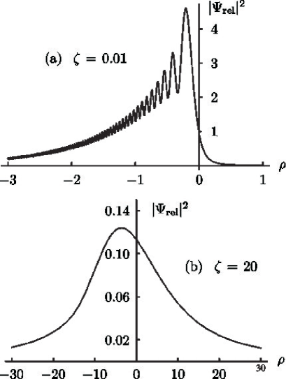
Figure 1: The relative-motion probability density $|\Psi_{\text{rel}}|^{2}$ (21) in dependence on $\rho=(r_{\text{rel}}-vt)/\Delta r_{\text{rel}}^{(0)}$ at (a) $\zeta=0.01$ and (b) $\zeta=20$.

so that $t_{\text{spr}}^{({\rm rel})}=\mu(\Delta r_{\text{rel}}^{(0)})^{2}/\hbar$ is the spreading time of the relative-motion wave packet. As the value of $|\Psi_{\text{rel}}|^{2}$ is concentrated around $r_{\text{rel}}\approx vt$, by putting $r_{\text{rel}}\approx vt$ in the definition of the parameter $\zeta$, we get $\zeta=t/t_{\text{spr}}^{({\rm rel})}$. In this form the meaning of $\zeta$ is obvious: it is the time after ionization measured in units of the spreading time of the relative-motion wave packet. In Figs. 1(a) and 1(b) the function $|\Psi_{\text{rel}}|^{2}$ is plotted in its dependence on $\rho\equiv(r_{\text{rel}}-vt)/\Delta r_{\text{rel}}^{(0)}$ at small and large $\zeta$’s respectively.

In the small-spreading regime ($\zeta\ll 1$) $|\Psi_{\text{rel}}|^{2}$ returns to the form of Eq. (20), but with additional oscillations on the left wing and a slightly smoothed right wing as compared to the step function jump of Eq. (20). In the large-spreading regime ($\zeta\gg 1$) $|\Psi_{\text{rel}}|^{2}$ takes a Lorentzian shape:

$$|\Psi_{\text{rel}}|^{2}=\frac{3}{8\pi^{2}}\frac{\cos^{2}\theta_{\text{rel}}}{r_{\text{rel}}^{2}}\frac{\Delta r_{\text{rel}}(t)}{(r_{\text{rel}}-vt)^{2}+\frac{1}{4}\left[\Delta r_{\text{rel}}(t)\right]^{2}},$$ (23)

where

$$\Delta r_{\text{rel}}(t)=\zeta\Delta r_{\text{rel}}^{(0)}=\frac{t}{t_{\text{spr}}}\Delta r_{\text{rel}}^{(0)}=v_{\text{spr}}t$$ (24)

and $v_{\text{spr}}\equiv\Delta r_{\text{rel}}^{(0)}/t_{\text{spr}}=\hbar/\mu\Delta r_{\text{rel}}^{(0)}$. Altogether, at small and large $\zeta$, the time-dependent width of the relative-motion wave packet is given by

$$\Delta r_{\text{rel}}(t)=\left\{\begin{array}[]{ll}\Delta r_{\text{rel}}^{(0)}=\displaystyle\frac{v}{2\gamma_{I}},&t\ll t_{{\rm spr}}^{({\rm rel})}\;(\zeta\ll 1);\\[14.22636pt] v_{\text{spr}}t=\displaystyle\frac{\hbar t}{\mu\Delta r_{\text{rel}}^{(0)}}=\displaystyle\frac{2\hbar\gamma_{I}}{\mu v}t,&t\gg t_{{\rm spr}}^{({\rm rel})}\;(\zeta\gg 1).\end{array}\right.$$ (25)

In spite of a difference between the Gaussian center-of-mass (8 ) and relative-motion [(20),(21), (23)] wave packets, their widths behave similarly: in dependence on $t$ they start from the initial values $\Delta r_{\text{cm}}^{(0)}$ and $\Delta r_{\text{rel}}^{(0)}$, and at time $t$ longer than the corresponding spreading time both $\Delta r_{\text{rel}}(t)$ (25) and $\Delta r_{\text{cm}}(t)$ (9) grow linearly. In both cases the spreading time is inversely proportional to the squared initial size and the velocity of spreading is inversely proportional to the initial size to the first power. The only qualitative difference concerns the mass of an objet: the total mass $M$ of the center-of-mass wave function is substituted by the reduced mass $\mu$ in the case of the relative-motion wave packet.

The relation between the center-of-mass and relative-motion wave packet widths can change with time due to different spreading velocities of these wave packets. This makes the time evolution of the electron-ion wave function rather complicated, and this problem will be discussed separately in Section V.

IV Localization of the electron-ion wave packet and entanglement

Before going further into details of time evolution, let us discuss the entanglement effect. As we will show, in cases of initially localized pairs of particles as in photoionization, and where significant further interaction is absent, entanglement can be evaluated by carrying out a series of localization measurements. This has a close analog in earlier studies of spontaneous photon emission with atom recoil JHE ; JHE2 ; SPIE as well as in the measurement-induced localization and entanglement discussed recently in a very different context by Rau, et al. RDK .

We will proceed by determining the dependence of entanglement on the ratio of widths

$$\eta(t)\equiv\frac{\Delta r_{\text{cm}}(t)}{\Delta r_{\text{rel}}(t)}$$ (26)

where the time $t$ is taken as a parameter. Note that in our treatment $\eta(t)$ is constrained only by momentum and energy conservation (e.g., we ignore final-state electron-ion Coulomb effects). Here $\Delta r_{\text{cm}}(t)$ is of kinematic origin whereas $\Delta r_{\text{rel}}(t)$ is due to the dynamics of the ionization process. We will see that $\eta(t)$ acts as the sole control parameter for entanglement of the two-particle system.

In accord with Eq. (4), the product of the wave functions Eqs. (8) and (21) determines the total wave function of the ion-electron system. It should now be considered as a function of ion and electron position vectors

$$\Psi(\vec{r}_{e},\vec{r}_{i},t)=\Psi_{\text{cm}}\left(\frac{m_{e}\vec{r}_{e}+m_{i}\vec{r}_{e}}{M},t\right)\times\Psi_{\text{rel}}(\vec{r}_{e}-\vec{r}_{i},t),$$ (27)

showing that both $\Psi$ and its squared absolute value are not factorable in the individual particle coordinates $\vec{r}_{e}$ and $\vec{r}_{i}$. Such non-factorization defines quantum particle entanglement of electron and ion.

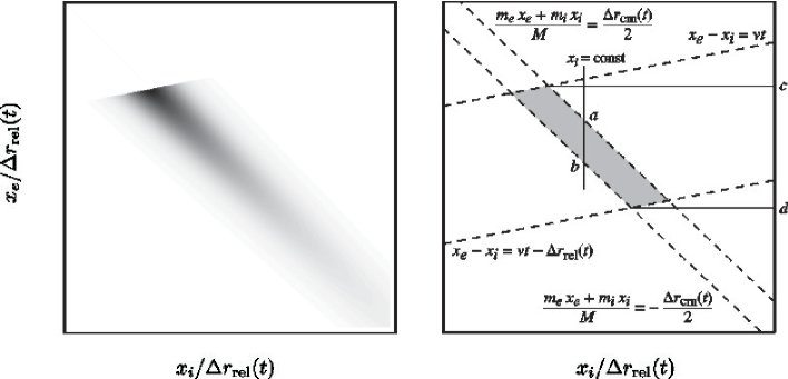
Figure 2: Views of the one-dimensional equivalent of $|\Psi|^{2}$ in Eq. (27). Here we illustrate the relation between entanglement and distribution of particle positions. High correlation between $x_{e}$ and $x_{i}$ can be attained only under the condition that the ranges of available $x_{e}$ and $x_{i}$ are large compared to the variation range of one of them at a fixed value of the other variable. We have used $m_{e}/m_{i}=0.2$, $\eta=0.5$, and $\gamma_{I}t=4$ for illustration. The dashed lines drawn in the figure tell approximately the region of localization of the wave function.

Now we focus on measurements appropriate for seeing entanglement. We need to distinguish coincidence and non-coincidence (single-particle) measurements, which have their theoretical counterparts in conditional and non-conditional probability distributions. For an example of a single-particle measurement, the electron probability distribution is measured regardless of the ion position (or vice versa). In contrast, a coincidence measurement assumes that a distribution of electron positions is registered while the ion detection position is kept at a given (constant) location (or vice versa). The difference between the results of coincidence and single-particle schemes of measurements is illustrated by Fig. 2. In this picture, in one dimension, we shade the region in which the joint probability density $|\Psi(\vec{r}_{e},\vec{r}_{i},t)|^{2}$ is significant. In the left plot the sharp leading edge of the theta function in Eq. (20) is apparent, with its long exponential tail, and one also sees the more abrupt Gaussian cut-off on the sides. A purely schematic view of the same thing is shown in the right plot, where artificially sharp dashed-line borders are introduced, and supposed to be determined by the localization zones of the relative-motion and center-of-mass wave functions.

Consider first an examination of the electron wave packet by the coincidence-scheme method, for a given ion coordinate $x_{i}=\text{const}$. The normalized measure of its width, $\Delta x_{e}/\Delta r_{\text{rel}}(t)$, will be given by the distance between the points marked $a$ and $b$. In contrast, the single-particle width takes into account the contributions from all possible different $x_{i}$’s. Thus a suitable measure of the single-particle width of the electron wave packet is given by the distance $cd$. It is obvious that the electron packet is relatively highly localized when $cd\gg ab$. Correspondingly, a horizontal line through the shaded region would provide a normalized measure of $\Delta x_{i}$, etc. From this sketch we formulate two conditions simultaneously necessary for entanglement to be large: a high aspect ratio of the shaded area and a nearly diagonal angle between the dashed lines restricting the wave packet localization zones and the coordinate axes $x_{e}$ and $x_{i}$. The high aspect ratio condition means that one of the two wave packets (${\rm``cm"}$ or ${\rm``rel"}$) is much wider than the other one.

Now we note that this relatively great localization condition is the same as a high entanglement condition. This becomes obvious by considering the two-particle wave packet $|\Psi(\vec{r}_{e},\vec{r}_{i},t)|^{2}$ as an information container Grobe-etal . Then the bibliography gets the added element:

Entanglement means that knowledge of one of the particles imparts information about the other, whereas non-entangled particles provide no information about each other. The greatest cross-specification of joint information by an entangled packet occurs when knowledge of one particle automatically corresponds to precise information about the other, i.e., knowledge of position $x_{i}$ strongly localizes the region where $x_{e}$ can be found. Reflection shows that a thin diagonal packet in $x_{i}$-$x_{e}$ space achieves this, and normalized relative information gain is well expressed by the ratio of single to coincidence width. Note that left or right inclination of the diagonal is immaterial. In contrast, in wave packet language the non-entangled condition (information about $x_{i}$ gives no information about $x_{e}$) is equivalent to a factored wave packet: $\Psi(x_{i},x_{e})\to\phi_{1}(x_{i})~{}\phi_{2}(x_{e})$. One sees that a sketch corresponding to Fig. 2, but for independent particles, has dashed lines that are horizontal and vertical, in which case all $x_{i}$’s predict exactly the same $\Delta x_{e}$, and vice versa.

Mathematically, single-particle probability densities are given by Eq. (27) integrated either over $\vec{r}_{i}$ or $\vec{r}_{e}$:

$$P_{e}(\vec{r}_{e},t)=\int d\vec{r}_{i}\ |\Psi(\vec{r}_{e},\vec{r}_{i},t)|^{2},$$ (28)

or

$$P_{i}(\vec{r}_{i},t)=\int d\vec{r}_{e}\ |\Psi(\vec{r}_{e},\vec{r}_{i},t)|^{2}.$$ (29)

Such distributions reveal no entanglement effects because all the information about the position of one of the particles is lost completely when the two-particle probability density is integrated over $\vec{r}_{i}$ or $\vec{r}_{e}$. However, $P_{e}$ and $P_{i}$ do serve a normalization role, as we explain later.

Let $\Delta r_{e}^{\text{(s)}}$ and $\Delta r_{i}^{\text{(s)}}$ be the widths of the single-particle electron and ion wave packets, where, for example, $|\Delta r_{e}^{\text{(s)}}|^{2}=\langle|\vec{r}_{e}|^{2}\rangle-|\langle\vec{r}_{e}\rangle|^{2}$, with

$$\langle\vec{r}_{e}\rangle = \int d\vec{r}_{e}\ \ \vec{r}_{e}\ P_{e}(\vec{r}_{e},t)$$ (30)

$$= \iint d\vec{r}_{e}\,d\vec{r}_{i}\ \ \vec{r}_{e}\ |\Psi(\vec{r}_{e},\vec{r}_{i},t)|^{2}$$

$$= \langle\vec{r}_{\text{cm}}\rangle+\frac{m_{i}}{M}\langle\vec{r}_{\text{rel}}\rangle$$

and

$$\langle\left|\vec{r}_{e}\right|^{2}\rangle = \int d\vec{r}_{e}\ \ r_{e}^{2}\ P_{e}(\vec{r}_{e},t)$$ (31)

$$= \iint d\vec{r}_{e}\,d\vec{r}_{i}\ \ r_{e}^{2}\ |\Psi(\vec{r}_{e},\vec{r}_{i},t)|^{2}$$

$$= \langle\left|\vec{r}_{\text{cm}}+\frac{m_{i}}{M}\vec{r}_{\text{rel}}\right|^{2}\rangle$$

$$= \langle\left|\vec{r}_{\text{cm}}\right|^{2}\rangle+2\frac{m_{i}}{M}\langle\vec{r}_{\text{cm}}\rangle\langle\vec{r}_{\text{rel}}\rangle+\frac{m_{i}^{2}}{M^{2}}\langle\left|\vec{r}_{\text{rel}}\right|^{2}\rangle.\hskip 22.76219pt$$

Note that we have used the relation $\vec{r}_{e}=\vec{r}_{\text{cm}}+\frac{m_{i}}{M}\vec{r}_{\text{rel}}$ and changed the integration variables to the center-of-mass and relative coordinates. Then Eqs. (30) and (31) yield the single-particle measures:

$$\delta r_{e}^{\text{(s)}}\equiv\frac{\Delta r_{e}^{\text{(s)}}}{\Delta r_{\text{rel}}(t)}=\sqrt{\eta^{2}(t)+\left(\frac{m_{i}}{M}\right)^{2}},$$ (32)

and, similarly,

$$\delta r_{i}^{\text{(s)}}\equiv\frac{\Delta r_{i}^{\text{(s)}}}{\Delta r_{\text{rel}}(t)}=\sqrt{\eta^{2}(t)+\left(\frac{m_{e}}{M}\right)^{2}}.$$ (33)

Note that the relative-motion wave packet width $\Delta r_{\text{rel}}(t)$ plays the role of a natural normalization factor for both single-particle and coincidence-scheme (see below) electron and ion wave packet widths. Divided by $\Delta r_{\text{rel}}(t)$ these widths become dimensionless, and they are denoted $\delta r_{e,i}^{\text{(s)}}$ and $\delta r_{e,i}^{\text{(c)}}$.

In the coincidence scheme of measurements the overall width of the distribution (27) with respect to $\vec{r}_{e}$ at a fixed $\vec{r}_{i}$ is given by the smaller of $(M/m_{e})\Delta r_{\text{cm}}(t)$ and $\Delta r_{\text{rel}}(t)$, which is well-represented by a simple formula for the coincidence measures:

$$\delta r_{e}^{\text{(c)}}\equiv\frac{\Delta r_{e}^{\text{(c)}}}{\Delta r_{\text{rel}}(t)}\approx\frac{\eta(t)}{\sqrt{\eta^{2}(t)+\left(\displaystyle\frac{m_{e}}{M}\right)^{2}}}.$$ (34)

The expression in Eq. (34) is a better approximation the closer we are to one of the extreme cases $(M/m_{e})\Delta r_{\text{cm}}(t)\gg\Delta r_{\text{rel}}(t)$ or $\ll\Delta r_{\text{rel}}(t)$. As shown later in this section, these limits correspond to the high entanglement regimes of main interest, and we do not need to bother too much about the details of the intermediate region. Similarly, at a given $\vec{r}_{e}$, the widths of $|\Psi_{\text{cm}}|^{2}$ and $|\Psi_{\text{rel}}|^{2}$ with respect to $\vec{r}_{i}$ are correspondingly $(M/m_{i})\Delta r_{\text{cm}}(t)$ and $\Delta r_{\text{rel}}(t)$. Therefore the overall width of $|\Psi|^{2}$ at a given $\vec{r}_{e}$ is the smaller of $(M/m_{i})\Delta r_{\text{cm}}(t)$ and $\Delta r_{\text{rel}}(t)$, corresponding to the formula

$$\delta r_{i}^{\text{(c)}}\equiv\frac{\Delta r_{i}^{\text{(c)}}}{\Delta r_{\text{rel}}(t)}\approx\frac{\eta(t)}{\sqrt{\eta^{2}(t)+\left(\displaystyle\frac{m_{i}}{M}\right)^{2}}}.$$ (35)

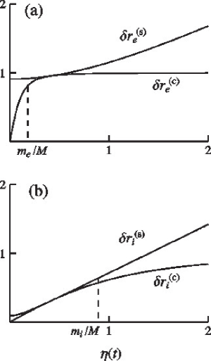
Figure 3: Electron (a) and ion (b) wave-packet widths in the schemes of single-particle and coincidence measurements with $m_{e}/m_{i}=0.1$.

It is clear now how $\eta(t)$ of Eq. (26) serves as a “control parameter” for both coincidence widths. Plots of $\delta r_{i}^{\text{(s)}}$ and $\delta r_{i}^{\text{(c)}}$ as a function of $\eta$, are shown in Fig. 3(a) whereas graphs of $\delta r_{i}^{\text{(s)}}$ and $\delta r_{i}^{\text{(c)}}$ are shown in Fig. 3(b). Note that we use in these graphs an artificial value of the electron to ion mass ratio $m_{e}/m_{i}=0.1$ so as to show more clearly the difference between the two curves for $\eta<1$. However, all the qualitative conclusions from these pictures remain the same for a more realistic value of this ratio $m_{e}/m_{i}\sim 10^{-4}$. One of these conclusions is that we always have $\delta r_{e,i}^{\text{(s)}}>\delta r_{e,i}^{\text{(c)}}$.

The ratios of single-to-coincidence electron and ion wave packet widths, $\delta r_{e,i}^{\text{(s)}}$ to $\delta r_{e,i}^{\text{(c)}}$, can be considered as a measure of entanglement, as remarked at the beginning of this section. As we will show elsewhere laterpaper , they are essentially identical to the corresponding Schmidt number discussed in earlier discussions of photon-atom entanglement JHE2 ; JHE . These ratios can be referred to as the electron and ion entanglement parameters in the form:

$$R_{e}\equiv\frac{\delta r_{e}^{\text{(s)}}}{\delta r_{e}^{\text{(c)}}}\quad\text{and}\quad R_{i}\equiv\frac{\delta r_{i}^{\text{(s)}}}{\delta r_{i}^{\text{(c)}}}.$$ (36)

Entanglement is large if $R_{e}\gg 1$ and/or $R_{i}\gg 1$. If $R_{e}\approx 1$ and $R_{i}\approx 1$, there is little or no entanglement at all.

By using Eqs. (32) – (35), we can find a useful approximate form of $R_{e}$ and $R_{i}$ :

$$R_{e}=R_{i}\approx\sqrt{\eta+\frac{1}{\eta}\left(\frac{m_{i}}{M}\right)^{2}}\sqrt{\eta+\frac{1}{\eta}\left(\frac{m_{e}}{M}\right)^{2}},$$ (37)

which is plotted in Fig. 4. Note that here the width ratios for the electron and the ion are the same, i.e., $R_{e}=R_{i}$. This is actually true only when the widths of $\Psi_{\text{cm}}$ and $\Psi_{\text{rel}}$ are very different from each other, or equivalently $\eta\gg 1$ or $\eta\ll 1$. Even though $R_{e}$ and $R_{i}$ may not be exactly the same in the zone $m_{e}/M<\eta<1$, they both have values around unity, which corresponds to the relatively less interesting small entanglement regime. Thus we designate the two of them together by $R$ without a subscript. The asymptotic behaviors of $R$ in three different regions of $\eta(t)$ are particularly noteworthy:

$$\text{Region 1},\ \ \eta\ll\frac{m_{e}}{M}\ll\displaystyle\frac{m_{i}}{M}:$$ (38)

$$R\sim\frac{m_{e}m_{i}}{M^{2}}\frac{\Delta r_{\text{rel}}(t)}{\Delta r_{\text{cm}}(t)}\sim\left(\frac{\mu}{M}\right)\frac{1}{\eta(t)};\qquad$$

$$\text{Region 2},\ \ \frac{m_{e}}{M}\ll\eta\ll\frac{m_{i}}{M}: R\sim 1;$$ (39)

$$\text{Region 3},\ \ \frac{m_{e}}{M}\ll\frac{m_{i}}{M}\ll\eta: R\sim\eta(t).$$ (40)

Note that the minimal value of the entanglement parameter (36) is equal to one, $R_{\min}=1$, and it is achieved at $\eta(t)=\sqrt{\mu/M}$.

V Time Evolution of Packet Widths and Entanglement Parameter

In Figs. 3 and 4 both the electron/ion wave packet widths and the entanglement parameters are shown, for fixed $t$, in their dependence on the control parameter defined earlier:

$$\eta(t)=\frac{\Delta r_{\text{cm}}(t)}{\Delta r_{\text{rel}}(t)}.$$ (41)

However, we can use the same pictures to show the time evolution of the widths $\Delta r_{e}(t)$ and $\Delta r_{i}(t)$ and the entanglement parameter $R(t)$ defined in (37). To do this, we have to learn how $\eta(t)$ changes with time.

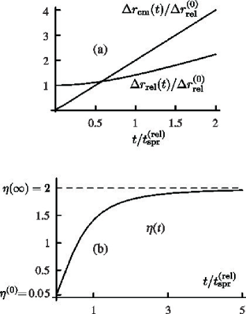
Figure 5: Part (a) shows the time-dependent widths of the center-of-mass and relative-motion wave packets (in units of $\Delta r_{\text{rel}}^{(0)}$), and part (b) shows the control parameter $\eta(t)$. We have taken $\eta_{0}=0.05$ and $m_{e}/M=0.1$.

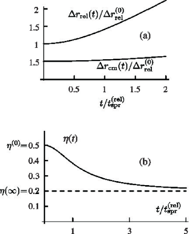
Figure 6: The same as in Fig. 5 but with $\eta_{0}=0.5$.

The two typical cases of significantly different behavior are illustrated in Figs. 5 and 6. Parts (a) and (b) of these Figures show the time dependence of the widths $\Delta r_{\text{cm}}(t)$ and $\Delta r_{\text{rel}}(t)$ themselves and of their ratio, which equals $\eta(t)$. A key feature of $\eta(t)$ is its strong dependence on the initial sizes of the center-of-mass and relative-motion wave packets, $\Delta r_{\rm cm}^{(0)}$ and $\Delta r_{\rm rel}^{(0)}$, or in other words, on the initial value of the control parameter $\eta(0)\equiv\eta_{0}$. Depending on its initial value, $\eta$ is either rising as shown in Fig. 5(a) or falling as in Fig. 6(b). The border between these two regimes is given by $\eta_{0}=\eta_{*}$, where

$$\eta_{*}\equiv\sqrt{\displaystyle\frac{\mu}{M}}.$$ (42)

If $\eta_{0}<\eta_{*}$, the center-of-mass wave packet spreads faster and eventually becomes wider than the relative-motion wave packet, though initially $\Delta r_{\rm cm}^{(0)}\ll\Delta r_{\rm rel}^{(0)}$. In this case the control parameter $\eta(t)$ is a monotonically growing function of $t$ (see Fig. 5(b)). On the contrary, if $\eta_{0}>\eta_{*}$, the center-of-mass wave packet spreads slower than the relative-motion wave packet. Though initially the center-of-mass packet can be either narrower or wider than the relative-motion packet, at very large $t$ the relative-motion packet becomes wider than the center-of mass packet. This gives rise to a falling function $\eta(t)$ shown in Fig. 6(b). In both cases ($\eta_{0}<\eta_{*}$ and $\eta_{0}>\eta_{*}$) the ranges of variation of the parameter $\eta(t)$ are finite. At very long times $\eta(t)$ has the asymptotic value

$$\eta\to\eta_{\infty}\equiv\frac{\mu}{M}\frac{1}{\eta_{0}},$$ (43)

which follows directly from the definition of $\eta$ (41) and Eqs. (9) and (25) for the widths $\Delta r_{\text{cm}}(t)$ and $\Delta r_{\text{rel}}(t)$. In the case $\eta_{0}=\eta_{*}$ the parameter $\eta(t)$ does not depend on time at all: $\eta(t)=const~{}(=\eta_{*}=\eta_{0}=\eta_{\infty})$.

By finding the evolution regimes for the control parameter $\eta(t)$, we can also make definite and interesting conclusions on the evolution of the entanglement parameter $R(t)$ (37). Directly from Eq. (37) one can easily see that for an arbitrary value of $\eta$, the entanglement parameter obeys the relation

$$R\left(\frac{1}{\eta}\;{\frac{\mu}{M}}\right)\equiv R(\eta).$$ (44)

The initial and final values of $\eta$ are connected with each other exactly by the same substitution as used in Eq. (44), we see that the initial and final values of the entanglement parameter must be equal:

$$R_{0}\equiv R_{\infty}=R(t\rightarrow\infty).$$ (45)

For the entanglement parameter given by Eq. (37) this equality is valid identically for all values of $\eta_{0}$. If $\eta_{0}$ is located in one of the high-entanglement regions of Fig. 4, $\eta_{0}\ll\mu/M$ as in (38), or $\eta_{0}\gg 1$ as in (40), the final value of $\eta$ is in the opposite of these two high-entanglement regions, $\eta_{\infty}\gg 1$ or $\eta_{\infty}\ll\mu/M$.

Thus we see that the time-dependent entanglement parameter $R(t)$ starts from a large value $R_{0}$, falls to $R\sim 1$ and then grows again to the same value from which it started. Physically such an evolution means that initially one of the wave packets is much wider than the other one, and for this reason the electron-ion entanglement is large. Then, as the narrower wave packet spreads faster, they become approximately of the same width, and this corresponds to a small entanglement. Finally, when the initially narrower but faster spreading wave packet outstrips the initially wider but slower spreading one, the relation between their widths reverses, and this returns us to the case of a large entanglement.

The difference between the cases $\eta_{0}\ll\mu/M$ and $\eta_{0}\gg 1$ concerns only the direction of evolution, correspondingly, to the right or to the left in the $\eta$-axis in Fig. 4. If the initial value of the parameter $\eta$ is located in the small-entanglement region (40), $\mu/M<\eta<1$, all the conclusions about the direction of evolution and about the relation between the initial and final values of the entanglement parameter remain valid. However, in this case, at all times $t$ the entanglement parameter remains on the order of one. If $\eta_{0}=\eta_{*}$, the entanglement parameter does not change at all, and $R(t)\equiv 1$.

VI Experimental Considerations

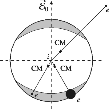
Figure 7: The new-moon shaded areas indicate the regions where the function $|\Psi_{\text{rel}}(\vec{r}_{e})|^{2}$ is relatively large,relatively large, i.e., at least as large as one-third the maximum value. Black dots indicate regions where $|\Psi_{\text{cm}}(\vec{r}_{e})|^{2}\neq 0$, at a given $\vec{r}_{i}$. Three shown experimental situations correspond to different locations of the electron detector, relative to the ion position, which defines the origin. A smaller size of such a black dot inside the shaded area corresponds to a higher level of entanglement. In the case when the black dot is located far outside of the shaded area, there is no overlapping between the center-of-mass and relative-motion wave functions and the total two-particle wave function equals zero, $\Psi=0$.

The discussion as given so far doesn’t treat some elements that will come into play in experimental tests. In order to bring them into focus briefly, we show in Fig. 7 what can be called experimentally realistic zones. We have plotted the region where the relative probability distribution is non-zero. It has a three-dimensional aspect that we do not need to show because it is axially symmetric about the polarization axis of the ionizing light beam, taken as the vertical axis here. It is not spherically symmetric because of the dipole character of photoionization (i.e., the factor $\vec{d}_{E_{*}0}\cdot\vec{\mathcal{E}}_{0}$ in Eq. (20)). The new-moon shaded areas indicate the regions where the relative-motion wave function $|\Psi_{\text{rel}}(\vec{r}_{e})|^{2}$ is relatively large.

Since the time evolution of the relative wave function is strictly limited by the step function $\theta(vt-r_{\text{rel}})$, we will here consider the ion position to define an origin of polar coordinates ($r_{i}\equiv 0$), in which case a circle of radius $r_{e}=vt$ limits the range of the electron coordinate at time $t$. The relative coordinate probability distribution $|\Psi_{\text{rel}}(\vec{r}_{e})|^{2}$ is of course not uniform inside this circle, so we have drawn the boundary on which $|\Psi_{\text{rel}}|^{2}$ equals $\frac{1}{3}$ of its maximum value. This creates two sectors with “new-moon” shape where there is the highest probability to find the electron, given that the ion is at the origin of the circle, and taking only $|\Psi_{\text{rel}}|^{2}$ into account. However, the probable position of the electron is also influenced by $|\Psi_{\text{cm}}(\vec{r}_{e})|^{2}$ at $\vec{r}_{i}\equiv 0$. In the figure the black dot regions show the range of electron positions given by $|\Psi_{\text{cm}}(\vec{r}_{e})|^{2}$ at different positions of the center of mass along the $r_{e}$-$r_{i}$ line.

The figure has many variations, and the sizes of the new-moon and $\Delta r_{e}$ zones change in time, as our formulas indicate. The overall shapes will remain the same, and a generic high-entanglement experiment will be one that ensures overlap between a small black-dot region and a high-probability portion of one of the new-moon regions (near the circle boundary). Higher count rate, although reduced entanglement, will be associated with increased size of the black dot region.

VII Photodissociation

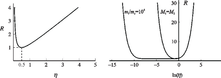
Figure 8: Entanglement parameter for two dissociating molecular fragments with $M_{1}=M_{2}$ (left) and the same dissociation curve plotted vs. ${\rm ln}(\eta)$ on the right, where the corresponding photoionization curve is included for comparison, with its very different mass ratio, $m_{i}=10^{4}m_{e}$.

It is easy to see that very similar results will arise in a treatment of photodissociation of molecules. Here we remark briefly on some of the differences. Let us assume that we consider a diatomic molecule undergoing dissociation. There will be a relevant dissociation rate $\gamma_{D}$, which can be substituted for the $\gamma_{I}$ governing ionization, and just as for the atom there will be an initial localization of the molecular center of mass. Then the main differences to the ionization example arise because the mass ratio of the fragments is much closer to 1. Compared to the case of photoionization, where $m_{e}\ll m_{i}$, the masses $M_{1}$ and $M_{2}$ of the photodissociation fragments obey $M_{1}\sim M_{2}$. Given this, the relative-motion velocity after dissociation $v\sim\sqrt{\hbar\omega/\mu}$ is significantly smaller than in the case of ionization (in atomic units $v_{\text{mol}}\sim\sqrt{\omega/M}$). The main difference between photoionization and photodissociation results concerns the region $\frac{\mu}{M}<\eta(t)<1$ of intermediate values of $\Delta r_{\text{cm}}(t)$ in Fig. 4 where $R\sim 1$. For $M_{1}=M_{2}=\frac{1}{2}M$ this region degenerates into a single point $\eta(t)=\frac{1}{2}=\eta_{*}$ (42). The entanglement coefficient $R$ is large both at $\eta(t)<\eta_{*}$ and $\eta(t)>\eta_{*}$. To show more clearly the difference between photoionization and photodissociation we plot in the right picture of Fig. 8 both molecular and atomic entanglement coefficients in their dependence on ${\rm ln}(\eta)$, with the electron to ion mass ration taking a realistic value $m_{e}/m_{i}=10^{-4}$. This picture shows that if in the case of photoionization there is a rather large region of intermediate values of $\eta$ where entanglement is small, $R\approx 1$, in the case of photodissociation of a molecule the entanglement parameter is large practically at any $\eta$ except one point $\eta=\eta_{*}$.

In dependence on time $t$ the control parameter $\eta(t)$ changes in a way similar to that described above for photoionization: $\eta(t)$ grows if initially it is small ($\eta_{0}<\eta_{*}$) and falls if large ($\eta_{0}>\eta_{*}$). The final value of the control parameter $\eta_{\infty}$ is related to $\eta_{0}$ by Eq. (43), which takes the form $\eta_{\infty}=1/(4\eta_{0})$. As shown previously, the initial and final values of the time-dependent entanglement parameter $R(t)$ are equal to each other, $R_{0}=R_{\infty}$. At $\eta_{0}=\eta_{*}$ both the control parameter $\eta(t)$ and the entanglement parameter $R(t)$ do not change with a varying time $t$, $\eta(t)\equiv\eta_{0}$ and $R(t)\equiv 1$. This is the only case when there is no entanglement at any time $t$. In all other cases ($\eta_{0}\neq\eta_{*}$) the entanglement parameter is large initially, reaches $R=1$ one at such $t$ that gives $\eta(t)=\eta_{*}$, and then grows again until it reaches its initial value $R_{0}$.

VIII Conclusion

We have evaluated the space-time behavior of the joint quantum state of an ion and electron following photoionization. Neglect of the incident photon momentum and of the final state Coulomb interaction means that the evolution of the state, and thus of the entanglement between the two particles, is constrained only by free-particle two-body momentum and energy conservation. This evolution provides an exactly calculable illustration of the situation involving massive particles sketched in the famous paper of Einstein, Podolsky, and Rosen EPR . We have obtained expressions for the entanglement-induced wave packet narrowing that occurs, and have indicated how entanglement can be identified and determined quantitatively. To do this we introduced $R$, the ratio between the entanglement-free wave packet width and the coincidence wave packet width. This is essentially the degree of entanglement. We gave expressions for $R$ in terms of ionization rate and packet spreading velocity, which are of course themselves determined by underlying parameters such as atomic bound-free dipole moments, relative electron and ion masses, ionizing field strength, etc. It was shown that $R$ depends in a simple way on the basic control parameter $\eta=\Delta r_{\text{cm}}(t)/\Delta r_{\text{rel}}(t)$, and can be much larger than unity in two limits, when $\eta\gg 1$ and also $\eta\ll 1$. The same formalism can be applied equally well to photodissociation of a diatomic molecule. For realistic physical values of the relevant parameters, in a typical example of atomic photoionization, $R$ is not very large because of the extreme discrepancy between $m_{i}$ and $m_{e}$, but for photodissociation of a diatomic molecule, where the fragment masses can be approximately equal, $R$ can be substantially increased.

IX Acknowledgements

The research reported here has been supported by the DoD Multidisciplinary University Research Initiative (MURI) program administered by the Army Research Office under Grant DAAD19-99-1-0215, by NSF grant PHY-0072359, Hong Kong Research Grants Council (grant no. CUHK4016/03P), and the RFBR grant 02-02-16400.

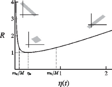
Figure 4: Plot of the entanglement parameter $R$ as a function of $\eta(t)$ with $m_{e}/m_{i}=0.1$; $\eta_{*}$ is the stability point (42) at which $\eta(t)\equiv const=\sqrt{\mu/M}$. The insets give the corresponding plots of the one-dimensional analog $|\Psi(x_{e},x_{i},t)|^{2}$ from Fig. 2. The axes of the three insets have been rescaled so as to show the details more clearly. The large entanglement regions are clearly seen to correspond to a large aspect ratio of the shadowed areas.

References

- (1) K. Gottfried, Quantum Mechanics (Benjamin, 1966), pp. 463-474.
- (2) M. V. Fedorov, Atomic and Free Electrons in a Strong Light Field (World Scientific, Singapore, 1997).
- (3) A. Einstein, B. Podolsky, and N. Rosen, Phys. Rev. 47, 777 (1935).
- (4) J. H. Eberly, K. W. Chan and C. K. Law, Phil. Trans. Roy. Soc. London A 361, 1519 (2003).
- (5) K. W. Chan, C. K. Law, and J. H. Eberly, Phys. Rev. Lett. 88, 100402 (2002); and also Phys. Rev. A 68, 022110 (2003).
- (6) H. Huang and J. H. Eberly, J. Mod. Opt. 40, 915 (1993); 43, 1891 (1996); C. K. Law, I. A. Walmsley and J. H. Eberly, Phys. Rev. Lett. 84, 5304 (2000).
- (7) M. D. Reid and P. D. Drummond, Phys. Rev. Lett. 60, 2731 (1988); M. D. Reid, Phys. Rev. A 40, 913 (1989).
- (8) T. Opatrny and G. Kurizki, Phys. Rev. Lett. 86, 3180 (2001)
- (9) L. D. Landau and E. M. Lifshitz, Quantum Mechanics (Pergamon Press, Oxford, 1977).
- (10) C. K. Law and J. H. Eberly, SPIE 5161, 27 (2003).
- (11) A. V. Rau, J. A. Dunningham, and K. Burnett, Science 301, 1081 (2003).
- (12) R. Grobe, K. Rzazewski and J.H. Eberly, J. Phys. B 27, L503 (1994).
- (13) Universal rules for quantification and measurement of bipartite entanglement, explicitly joining the Schmidt context to localization measurements, will be treated in a wider context elsewhere.