Quantum averaging and resonances:
two-level atom in a one-mode quantized field

Abstract

We construct a non-perturbative approach based on quantum averaging combined with resonant transformations to detect the resonances of a given Hamiltonian and to treat them. This approach, that generalizes the rotating-wave approximation, takes into account the resonances at low field and also at high field (non-linear resonances). This allows to derive effective Hamiltonians that contain the qualitative features of the spectrum, i.e. crossings and avoided crossings, as a function of the coupling constant. At a second stage the precision of the spectrum can be improved quantitatively by standard perturbative methods like contact transformations. We illustrate this method to determine the spectrum of a two-level atom interacting with a single mode of a quantized field.

I Introduction

Some important features of classical and quantum systems are determined by resonances of the system which can not be treated by perturbative approaches. In the vicinity of resonances the perturbative formulas display small denominators that lead to the divergence of the perturbative expansions. A widely used model that incorporates a one-photon resonance is the Jaynes-Cummings Hamiltonian extracted from the full dressed Hamiltonian that describes a two-level system coupled with a single mode of a quantized field Jaynes and Cummings (1963). Its counterpart for an interaction with a semi-classical laser field is the RWA Hamiltonian (rotating-wave approximation) Shirley (1965).

In this article we give a systematic method that allows to construct effective Hamiltonians and determine their spectrum by treating the resonances with an adaptation of resonant transformations that were introduced in Ref. Jauslin et al. (2000) in the context of laser-driven quantum systems in the Floquet representation. The goal is to obtain the spectrum for a whole interval of values of a parameter like the coupling constant. This is needed e.g. in applications where the coupling changes adiabatically Guérin and Jauslin (2003), corresponding e.g. to envelopes of laser pulses or to transversal spatial profiles of cavity fields. The method is based on the detection of resonances by a projector derived from Quantum Averaging (QA). We illustrate it on the problem of a two-level atom interacting with a quantized field and show that a treatment of all the relevant resonances of the system in a given range of parameters allows to reproduce with good accuracy the spectrum of this system. The treatment of the resonances yields the qualitative structure of the spectrum – the crossings and avoided crossings – as a function of the coupling constant. Once this main structure is obtained, one can systematically improve the quantitative accuracy of the spectrum by applying perturbative methods. We use contact transformations with a Kolmogorov-Arnold-Moser (KAM) iteration Jauslin et al. (2000), that are particularly efficient due to its superconvergent properties.

The paper is structured as follows. In Section II, we describe the method of resonance analysis and the construction of effective Hamiltonians. Section III contains the presentation of the model and some preliminary considerations. In Section IV, taking into account the resonances of this model in the weak-coupling regime, we extract the effective Hamiltonians by quantum averaging techniques and resonant transformations. In the weak-coupling regime we have to iterate this procedure several times to derive the essential structure of the spectrum in larger ranges of the coupling constant. In Sec.V we extract the effective Hamiltonians in the strong-coupling regime where the qualitative properties of the spectrum can be globally obtained by some preliminary unitary transformations and one resonant transformation which treats the zero-field resonances. We obtain an accurate approximation valid for all values of the coupling constant that contains all the qualitative structure. Finally, in Sec.VI we give some conclusions.

II principle of the method

We consider a Hamiltonian $H=H_{0}+\epsilon V$ where $H_{0}$ is the unperturbed Hamiltonian, $\epsilon V$ is the perturbation and $\epsilon$ is an ordering parameter. The first analysis of this problem is in terms of perturbation theory: we look for a KAM-type unitary transformation $e^{\epsilon W}$ close to the identity that allows to reduce the order of the perturbation from $\epsilon$ to $\epsilon^{2}$:

$$e^{-\epsilon W}He^{\epsilon W}=H_{0}+\epsilon D+\epsilon^{2}V_{2}.$$ (1)

$\epsilon D$ is a remaining term of order $\epsilon$ that satisfies $\left[H_{0},D\right]=0$. The unknown $W$ and $D$ are solutions of the following equations Bellissard (1985); Jauslin et al. (2000)

$$\left[H_{0},W\right]+V = D,$$ (2a)

$$\left[H_{0},D\right] = 0.$$ (2b)

The remaining perturbation of order $\epsilon^{2}$ is given by

$$\epsilon^{2}V_{2}=\sum_{m=2}^{\infty}\frac{\epsilon^{m}}{m!}~{}\left((m-1)L^{m-1}_{W}V+L^{m-1}_{W}D\right),$$ (3)

where $L_{W}$ is defined as

$$L_{W}B=\left[B,W\right].$$ (4)

The solutions of Eqs.(2) can be written in terms of averaging Primas (1963); Jauslin et al. (2000):

$$D = \overline{V}\equiv\Pi_{H_{0}}V:=\lim_{\tau\to\infty}\frac{1}{\tau}\int_{0}^{\tau}dse^{-iH_{0}s}Ve^{iH_{0}s}$$ (5a)

$$= \sum_{\nu,j,j^{\prime}}|\nu,j\rangle\langle\nu,j|V|\nu,j^{\prime}\rangle\langle\nu,j^{\prime}|,$$

$$W = \lim_{\tau\to\infty}\frac{-i}{\tau}\int_{0}^{\tau}ds\int_{0}^{s}ds^{\prime}~{}e^{-iH_{0}s^{\prime}}(V-\Pi_{H_{0}}V)e^{iH_{0}s^{\prime}}$$ (5b)

$$= -\sum_{\nu,j,j^{\prime},\nu^{\prime}\neq\nu}\frac{|\nu,j\rangle\langle\nu,j|V|\nu^{\prime},j^{\prime}\rangle\langle\nu^{\prime},j^{\prime}|}{E_{\nu}^{(0)}-E_{\nu^{\prime}}^{(0)}},$$

where $\nu$ labels the different eigenvalues $E_{\nu}^{(0)}$ of $H_{0}$, and $j$ is a degeneracy index which distinguishes different basis vectors $|\nu,j\rangle$ of the degeneracy eigenspace. The operator $\Pi_{H_{0}}$ is the projector on the kernel of the application $A\mapsto[H_{0},A]$. We remark that the integral representation of $D,W$ in Eqs. (5) can be also well-defined in cases where $H_{0}$ has a continuum spectrum. The units are chosen such that $\hbar=1$. In the following discussion, we do not write explicitly the ordering parameter $\epsilon$.

A resonance is defined as a degeneracy of an eigenvalue $E_{\nu}^{(0)}$ of $H_{0}$ and is said to be active if the perturbation V has nonzero matrix elements in the degeneracy subspace of $E_{\nu}^{(0)}$: $\langle\nu,j|V|\nu,j^{\prime}\rangle\neq 0$  for some $j,j^{\prime}$. Otherwise the resonance is called passive or mute. An active resonance renders $W$ arbitrarily large close to the degeneracy and makes the perturbative expansion diverge. The method we present here, is a construction designed to avoid such divergences. We remark that the concept of resonance is defined intrinsically for $H_{0}$, while the distinction between active and passive depends on the relation between $H_{0}$ and $V$. The analysis of the resonances involves thus three aspects:

• Decomposition of the Hamiltonian into $H=H_{0}+V$. Different decompositions can be considered for different regimes of the parameters of $H$.

• Determination of degenerate eigenvalues of $H_{0}$.

• Detection of the resonant terms in the perturbation $V$ that couple these degenerate eigenstates.

The resonant terms of $V$ can be detected by projectors of type $\Pi_{H_{0}}$ that extract a block-diagonal part of $V$ relative to $H_{0}$, where the blocks are generated by the degeneracy subspaces. In absence of active resonances, when all the eigenvalues of $H_{0}$ are non-degenerate or when the resonances are mute, the matrix representation of $\Pi_{H_{0}}V$ is in fact diagonal in the eigenbasis of $H_{0}$. In presence of active resonances, the block-diagonal effective Hamiltonian that takes into account the considered resonance of the original Hamiltonian can be written as

$$H^{\text{eff}}=H_{0}+\Pi_{H_{0}}V.$$ (6)

We will call the transformation that diagonalizes $H^{\text{eff}}$ Resonant Transformation (RT). The Hamiltonian $H=H^{\text{eff}}+(V-\Pi_{H_{0}}V)$ is transformed under RT (denoted $\mathcal{R}$) as follows:

$$H_{1}=\mathcal{R}^{{\dagger}}H\mathcal{R} = \mathcal{R}^{{\dagger}}H^{\text{eff}}\mathcal{R}+\mathcal{R}^{{\dagger}}(V-\Pi_{H_{0}}V)\mathcal{R}$$ (7)

$$=: H_{1}^{(0)}+V_{1},$$

where $H_{1}^{(0)}$ is defined as the new renormalized reference Hamiltonian and $V_{1}$ is the new perturbation. If $H_{1}^{(0)}+V_{1}$ does not have any other active resonance in the considered range of the coupling constant, we can at a second stage improve the spectrum by a KAM-type perturbative expansion which is expected to converge. If there are other active resonances, we have to iterate the renormalization procedure by applying another RT. We remark that there are cases of multi-photon resonances where the resonant terms appear only after applying one or several contact transformations.

III description of the model and preliminary considerations

We consider as an illustration a two-level atom interacting with a single mode of a quantized field described by

$$H=\omega(a^{{\dagger}}a+1/2)\otimes\openone_{2}+\frac{\omega_{0}}{2}\openone\otimes\sigma_{z}+g(a+a^{{\dagger}})\otimes\sigma_{x},$$ (8)

where $a$, $a^{{\dagger}}$ are the annihilation and creation operators for the field mode with the commutation relation $[a,a^{{\dagger}}]=\openone=\sum_{n=0}^{\infty}|n\rangle\langle n|$ , $\sigma_{z},\sigma_{x}$ are Pauli matrices and $\openone_{2}$ is the $2\times 2$ identity matrix. Here $\omega$ is the frequency of field mode, $\omega_{0}$ is the energy difference of the two atomic states and $g$ is the dipole-coupling between the field mode and the atom. This Hamiltonian acts on the Hilbert space $\mathcal{K}=\mathcal{F}\otimes\mathcal{H}$ where $\mathcal{H}=\mathbb{C}^{2}$ is the Hilbert space of the atom generated by $|\pm\rangle$ (eigenvectors of $\sigma_{z}$) and $\mathcal{F}$ is the Fock space of the field mode generated by the orthonormal basis $\{|n\rangle~{};~{}n=0,1,2,\cdots\}$, $n$ being the photon number of the field.

For this system there is a parity operator

$$P=e^{i\pi a^{{\dagger}}a}\otimes\sigma_{z}=\sum_{n=0}^{\infty}(-1)^{n}|n\rangle\langle n|\otimes\sigma_{z},$$ (9)

with the properties

$$[P,H]=0,~{}~{}~{}~{}P=P^{{\dagger}},~{}~{}~{}~{}P^{2}=\openone_{\mathcal{K}}\equiv\openone\otimes\openone_{2}.$$ (10)

As a consequence, the eigenstates of $H$ can be separated into two symmetry classes, even or odd, under $P$:

$$P|\phi_{n,\pm}\rangle=\pm|\phi_{n,\pm}\rangle,~{}~{}~{}~{}H|\phi_{n,\pm}\rangle=E_{n,\pm}|\phi_{n,\pm}\rangle.$$ (11)

The parity operator also commutes with any operator that depends only on $N=a^{{\dagger}}a$ and $\sigma_{z}$.

In spite of the simple form of (8), its exact solutions are not known. This can be related to the fact that the classical limit of this model is non-integrable Milonni et al. (1983). This model is of great interest as a physical model in quantum optics Allen and Eberly (1975); Lais and Steimle (1990); Cohen-Tannoudji et al. (1992); Frasca (2002) and quantum chaos Graham and Höhnerbach (1984a, b). Some approximate solutions of this model have been studied among many others in Franchuk et al. (1996); Tur (2000) using different formalisms.

The conceptual framework for the solution of this system based on the construction of unitary transformations can be described as follows: First, we decompose the Hamiltonian in two terms as $H=H_{0}+V$. Depending on the considered ranges of the parameters of the system, different decompositions may be considered. $H_{0}$ is a priori an operator that is a regular function exclusively of the operators $N$ and $\sigma_{z}$. The operators $N$ and $\sigma_{z}$ can be considered in the present model as quantum analogues of classical global actions Weigert and Müller (1995), and $H_{0}$ can be labelled integrable. The perturbation $V$ contains functions that involve also the other operators $a,a^{{\dagger}},\sigma_{x},\sigma_{y}$. The goal is to determine a unitary transformation $U$, that should be expressed in terms of well-behaved regular functions of $a,a^{{\dagger}},\sigma_{x},\sigma_{y},\sigma_{z}$, such that:

$$U^{{\dagger}}\left(H_{0}(N,\sigma_{z})+V(a,a^{{\dagger}},\sigma_{x},\sigma_{y},\sigma_{z})\right)U=H^{\prime}(N,\sigma_{z}),$$ (12)

where $H^{\prime}$ is a regular function $f$ exclusively of the action operators $N,\sigma_{z}$: $H^{\prime}(N,\sigma_{z})=f(N,\sigma_{z})$. With this transformation the eigenvectors of $H$ can be expressed as $|\phi_{n,\pm}\rangle=U(|n\rangle\otimes|\pm\rangle)$ and the corresponding eigenvalues as $E_{n,\pm}=f(n,\pm 1)$ where $N|n\rangle=n|n\rangle$ and $\sigma_{z}|\pm\rangle=\pm|\pm\rangle$.

We remark that in our context the important property for singling out the operators $N,\sigma_{z}$ is that they commute with each other and their spectrum and eigenvectors are explicitly available. The question of whether for a given model there exists a regular unitary transformation $U$ that accomplishes the above requirement is, to our knowledge, an open problem.

Most of the perturbative approaches can be interpreted as methods to find approximations of the transformation $U$. The presence of resonances is one of the central difficulties in the construction of $U$, as will be made precise below. In this paper we discuss an iterative approach that consists of constructing first some approximations of $U$ that take into account the dominating effects of a certain number of resonances. The transformations involved in this stage are far from the identity and have a clearly non-perturbative character. Once we have a transformation that takes into account the main effect of a set of resonances that are relevant in a considered interval of the coupling constant $g$, a perturbative approach (like the KAM, Van Vleck, or other types of the contact transformation) can be applied to improve the approximation quantitatively. The transformations involved in this second stage can be considered as deformations of the identity, since they can be written in the form $e^{W}$. This stage cannot be implemented if the resonances are not taken care of beforehand. Indeed the perturbative formulations diverge close to resonances due to the appearance of small denominators as can be seen in Eq. (5-b).

As in classical mechanics, the construction of the transformation $U$ leading to a Hamiltonian that contains only action variables can often be considered in two steps: $U=U_{1}U_{2}$. In the first step, that is called reduction, the Hamiltonian is transformed by $U_{1}$ into a form that contains functions of $\sigma_{z},\sigma_{x},\sigma_{y}$ and $N$, but not of $a$ and $a^{{\dagger}}$. The degree of freedom of the field is made trivial and the number of non-trivial degrees of freedom is thus reduced by one. When we apply this reduction to the effective Hamiltonian (6), we obtain a reduced effective Hamiltonian. We remark that in the literature, this “reduced effective Hamiltonian” is often called simply “effective Hamiltonian”. In the second step, the reduced Hamiltonian is transformed under $U_{2}$ into a form that contains functions of only $N$ and $\sigma_{z}$. For the model (8), the reduction step corresponds to diagonalization in the Fock space and the second step corresponds to diagonalization in the atomic Hilbert space which in this case is trivial. The construction of the RT is based on this reduction procedure.

IV effective Hamiltonians in the weak-coupling regime

In this section we consider the Hamiltonian (8) at resonance $\omega_{0}=\omega$ in the weak coupling regime, so that $H$ can be decomposed as follows:

$$H = H_{0}+V,$$

$$H_{0}(N,\sigma_{z}) = \omega(N+1/2)\otimes\openone_{2}+\frac{\omega_{0}}{2}\openone\otimes\sigma_{z},$$

$$V(a,a^{{\dagger}},\sigma_{x},g) = g(a+a^{{\dagger}})\otimes\sigma_{x}.$$ (13)

The eigenvalues and eigenvectors of $H_{0}$ are:

$$E_{n,\pm}^{(0)} = \omega(n+1/2)\pm\omega_{0}/2,$$

$$|\phi_{n,\pm}^{(0)}\rangle = |n,\pm\rangle=|n\rangle\otimes|\pm\rangle,$$

$$|n,+\rangle = \left(\begin{array}[]{c}|n\rangle\\ 0\\ \end{array}\right),~{}~{}~{}~{}|n,-\rangle=\left(\begin{array}[]{c}0\\ |n\rangle\\ \end{array}\right).$$ (18)

For $\omega_{0}=\omega$ there is a one photon resonance which corresponds to the degeneracies $E_{n,+}^{(0)}=E_{n+1,-}^{(0)}$. The degeneracy eigenspaces are spanned by the vectors $|\phi_{n,+}^{(0)}\rangle$ and $|\phi_{n+1,-}^{(0)}\rangle$. The resonant part of $V$ is obtained by (5-a):

$$V_{res}:=\Pi_{H_{0}}V = \sum_{n=0}^{\infty}\big{(}|n,+\rangle\langle n,+|V|n+1,-\rangle\langle n+1,-|$$ (21)

$$+ |n+1,-\rangle\langle n+1,-|V|n,+\rangle\langle n,+|\big{)}$$

$$= g\left(\begin{array}[]{cc}0&a\\ a^{{\dagger}}&0\\ \end{array}\right),$$

where we have used the relations

$$a=\sum_{n=0}^{\infty}\sqrt{n+1}~{}|n\rangle\langle n+1|,~{}~{}~{}~{}~{}~{}a^{{\dagger}}=\sum_{n=0}^{\infty}\sqrt{n+1}~{}|n+1\rangle\langle n|.$$ (22)

The effective Hamiltonian containing the one-photon resonance is the so-called Jaynes-Cummings Hamiltonian that can be written as

$$H_{0}^{\text{eff}} = H_{JC}=H_{0}+\Pi_{H_{0}}V=\omega(N+1/2)\otimes\openone_{2}$$ (25)

$$+ \frac{\omega}{2}\openone\otimes\sigma_{z}+g\left(\begin{array}[]{cc}0&a\\ a^{{\dagger}}&0\\ \end{array}\right).$$

$H_{JC}$ is a good approximation of (8) for low energies in the limit $g\ll\omega_{0},|~{}\omega-\omega_{0}|\ll\omega_{0}$. In this limit, the so-called counter-rotating terms $g\left(\begin{array}[]{cc}0&a^{{\dagger}}\\ a&0\\ \end{array}\right)$ can be discarded (rotating-wave approximation). $H$ can thus be written as $H=H_{0}^{\text{eff}}(N,a,a^{{\dagger}},\sigma_{x},\sigma_{y};g)+(V-\Pi_{H_{0}}V)$. Next we transform $H_{0}^{\text{eff}}$ by a resonant transformation $\mathcal{R}_{1}$ to a regular function of exclusively the action operators $N,\sigma_{z}$. Every resonant transformation is performed in two steps. To diagonalize $H_{0}^{\text{eff}}$ in the Fock space (the reduction step of the RT denoted $R_{1}$) we define a transformation in such a way that the following condition is satisfied:

$$R_{1}^{{\dagger}}V_{res}R_{1}=f(N)\otimes\sigma_{x},$$ (26)

where $f$ is a regular function of $N$ which has to be determined. We require furthermore that $R_{1}^{{\dagger}}H_{0}R_{1}$ stays a function of only $N$ and $\sigma_{z}$. A suitable transformation satisfying these conditions is

$$R_{1}:=\left(\begin{array}[]{cc}(aa^{{\dagger}})^{-1/2}a&~{}~{}0\\ 0&~{}~{}\openone\\ \end{array}\right)\equiv\left(\begin{array}[]{cc}\sum_{n=0}^{\infty}|n\rangle\langle n+1|&~{}~{}0\\ 0&~{}~{}\openone\\ \end{array}\right).$$ (27)

This transformation is not unitary but isometric Reed and Simon (1980):

$$R_{1}R_{1}^{{\dagger}}=\openone_{\mathcal{K}}~{}~{},~{}~{}R_{1}^{{\dagger}}R_{1}=\openone_{\mathcal{K}}-\left(\begin{array}[]{cc}|0\rangle\langle 0|&~{}~{}0\\ 0&~{}~{}0\\ \end{array}\right),$$ (28)

where we have used the identity $a^{{\dagger}}(N+1)^{-1}a=\openone-|0\rangle\langle 0|$. Applying this transformation on the resonant term gives

$$R_{1}^{{\dagger}}V_{res}R_{1}=g~{}a^{{\dagger}}(aa^{{\dagger}})^{-1/2}a\otimes\sigma_{x}=g\sqrt{N}\otimes\sigma_{x}$$ (29)

and $H$ is transformed under $R_{1}$ as

$$H_{R_{1}}=R_{1}^{{\dagger}}HR_{1}=\omega N\otimes\openone_{2}+g\sqrt{N}\otimes\sigma_{x}+g\left(\begin{array}[]{cc}0&~{}~{}A^{{\dagger}}\\ A&~{}~{}0\\ \end{array}\right),$$ (30)

where

$$A=a(aa^{{\dagger}})^{-1/2}a=\sum_{n=0}^{\infty}\sqrt{n+1}~{}|n\rangle\langle n+2|,$$ (31)

with the properties:

$$AA^{{\dagger}}=aa^{{\dagger}}~{}~{},~{}~{}A^{{\dagger}}A=a^{{\dagger}}a-\openone+|0\rangle\langle 0|.$$ (32)

To each eigenvector $|\phi\rangle$ of $H$ corresponds an eigenvector $R_{1}^{{\dagger}}|\phi\rangle$ of $H_{R_{1}}$, since:

$$H_{R_{1}}R_{1}^{{\dagger}}|\phi\rangle=R_{1}^{{\dagger}}HR_{1}R_{1}^{{\dagger}}|\phi\rangle=\lambda R_{1}^{{\dagger}}|\phi\rangle.$$ (33)

We remark that $R_{1}^{{\dagger}}|\phi\rangle\neq 0~{}~{}\forall|\phi\rangle\in\mathcal{K}$. Every eigenvalue of the original Hamiltonian $H$ is also an eigenvalue of the transformed Hamiltonian $H_{R_{1}}$. However since $R_{1}|0,+\rangle=0$, there is a difference in the spectrum between $H$ and $H_{R_{1}}$ : $H_{R_{1}}$ has an extra zero eigenvalue with eigenvector $|0,+\rangle$. The spurious eigenvalue can be detected and eliminated after applying the transformation. Indeed, since $|0,+\rangle$ is not coupled to any vector in its orthogonal complement, one can eliminate it from the rest of the calculation by taking the projection of $H_{R_{1}}$ into the orthogonal complement $H_{R_{1},\bot(0,+)}=P_{\bot(0,+)}H_{R_{1}}P_{\bot(0,+)}$ with $P_{\bot(0,+)}=\openone_{\mathcal{K}}-|0,+\rangle\langle 0,+|$.This difference between unitary and isometric transformations was not taken into account in Bérubé-Lauzière et al. (1994) in diagonalizing the Jaynes-Cummings Hamiltonian.

The second step of the RT is the diagonalization of $R_{1}^{{\dagger}}H_{0}^{\text{eff}}R_{1}=\omega N\otimes\openone_{2}+\sqrt{N}\otimes\sigma_{x}$ in the atomic Hilbert space. This can be performed by a $\pi/2$ rotation around the y-axis:

$$T=e^{-i\frac{\pi}{4}\sigma_{y}}=\frac{1}{\sqrt{2}}\left(\begin{array}[]{cc}1&-1\\ 1&1\\ \end{array}\right),$$ (34)

with the properties

$$T^{{\dagger}}\sigma_{x}T=\sigma_{z},~{}~{}~{}~{}T^{{\dagger}}\sigma_{z}T=-\sigma_{x}.$$ (35)

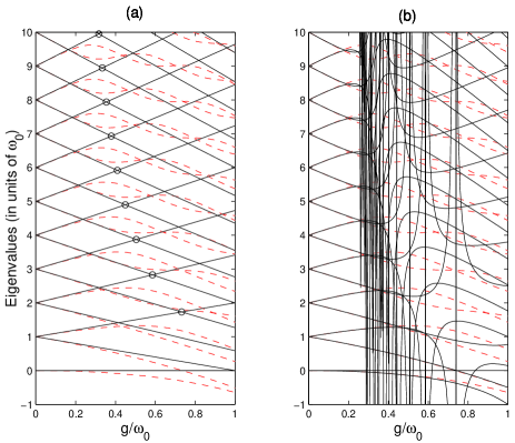
Figure 1: Comparison of exact numerical eigenvalues (dashed lines) of (8) for one-photon resonance $\omega=\omega_{0}$ with the approximate ones (solid lines) obtained after (a) 1 one-photon RT given by (47), (b) 1 one-photon RT plus 1 iteration of KAM-type perturbative expansion. The divergence observed around $g/\omega_{0}=0.3$ in panel (b) is due to the active nonlinear resonances of $H_{1}^{(0)}$ occurred at the degeneracies marked by circles in panel (a). One can see clearly that the locations of these resonances depend on $n$ according to Eq. (48).

However, since the spurious eigenvector $|0,+\rangle$ can be separated and $|0,-\rangle$ is already an eigenvector of $R_{1}^{{\dagger}}H_{0}^{\text{eff}}R_{1}$, the transformation $T$ must be applied only on the subspace with $n\geq 1$ photons. The complete transformation (denoted $T_{1}$) reads thus

$$T_{1}=P_{0}\otimes\openone_{2}+P_{\bot 0}\otimes T,$$ (36)

where

$$P_{0}=|0\rangle\langle 0|,~{}~{}~{}~{}P_{\bot 0}=\sum_{n=1}^{\infty}|n\rangle\langle n|.$$ (37)

Applying $T_{1}$ gives

$$H_{1} := T_{1}^{{\dagger}}R_{1}^{{\dagger}}HR_{1}T_{1}$$ (38)

$$= H_{1}^{(0)}(N,\sigma_{z};g)+V_{1}(a,a^{{\dagger}},\sigma_{z},\sigma_{x},\sigma_{y};g),$$

with

$$H_{1}^{(0)} = \omega N\otimes\openone_{2}+g\sqrt{N}\otimes\sigma_{z},$$

$$V_{1} = g/2\left(\begin{array}[]{cc}A_{\bot 0}+A_{\bot 0}^{{\dagger}}&~{}~{}-A_{\bot 0}+A_{\bot 0}^{{\dagger}}\\ A_{\bot 0}-A_{\bot 0}^{{\dagger}}&~{}~{}-A_{\bot 0}-A_{\bot 0}^{{\dagger}}\\ \end{array}\right)$$ (41)

$$+ \frac{g}{\sqrt{2}}\left(\begin{array}[]{cc}0&~{}~{}|2\rangle\langle 0|\\ |0\rangle\langle 2|&~{}~{}-|2\rangle\langle 0|-|0\rangle\langle 2|\\ \end{array}\right),$$ (44)

where

$$A_{\bot 0}=P_{\bot 0}AP_{\bot 0}=\sum_{n=1}^{\infty}\sqrt{n+1}~{}|n\rangle\langle n+2|,$$ (45)

and use has been made of the relations

$$AP_{0}=P_{0}A^{{\dagger}}=0,~{}~{}~{}~{}P_{0}AP_{\bot 0}=|0\rangle\langle 2|.$$ (46)

The first RT, is thus the combination of $R_{1}T_{1}$. Since the transformation $R_{1}$ dresses the upper atomic state by (–1) photon Cohen-Tannoudji et al. (1992), $\mathcal{R}_{1}=R_{1}T_{1}$ can be called a one-photon RT.

$H_{1}^{(0)}$ is in fact the diagonalized Jaynes-Cummings Hamiltonian in the resonant case with the eigenvalues

$$E_{1,(n,\pm)}^{(0)}(g)=\omega n\pm g\sqrt{n},~{}~{}~{}~{}n=0,1,2,\cdots.$$ (47)

The eigenvalues and therefore the degeneracies of $H_{1}^{(0)}$ depend on the coupling constant $g$. For small enough $g$ and low energies, $H_{1}^{(0)}$ does not have other degeneracies besides the ones at $g=0$ for which the new perturbation $V_{1}$ does not have resonant terms, and we can apply KAM-type transformations to improve quantitatively the precision of the spectrum by iteration. A single KAM transformation (which is essentially equivalent to second order perturbation theory) already gives quite good precision, as shown in Fig. (1-b) for $g/\omega_{0}<0.25$ for energies smaller than $10\omega_{0}$. If we take large enough $g$ or larger energies, we encounter new resonances which appear at some specific finite values of $g$. These resonances are called field-induced resonances or nonlinear resonances. For larger values of the coupling ($g/\omega_{0}\approx 0.3$ for the shown energy interval in Fig. (1-b)), where we encounter nonlinear resonances, the KAM iteration diverges. The eigenvalues of $H_{1}^{(0)}$ are degenerate at $g_{n}=\omega/(\sqrt{n}+\sqrt{n+1})$ as $E_{1,(n,+)}^{(0)}(g_{n})=E_{1,(n+1,-)}^{(0)}(g_{n})$. But the corresponding resonant terms in $V_{1}$ are zero due to parity (mute resonances). The next degeneracies appear at

$$g_{n}=2\omega/(\sqrt{n}+\sqrt{n+2}),$$ (48)

as

$$E_{1,(n,+)}^{(0)}(g_{n})=E_{1,(n+2,-)}^{(0)}(g_{n}),$$ (49)

which have been marked by circles in figure (1-a). All the other resonances are mute. There is an infinite family of nonlinear resonances located at different values of the coupling $g_{n}$. We observe from (48) that for higher energies the nonlinear resonances appear for arbitrary small coupling ($\lim_{n\rightarrow\infty}g_{n}=0$). We can extract the resonant terms corresponding to the whole family in a single step by working with the combined projector $\sum_{n}\Pi_{H_{1}^{(0)}(g_{n})}$. The resonant terms in $V_{1}$ corresponding to the degeneracies (49) are

$$\sum_{n}\Pi_{H_{1}^{(0)}(g_{n})}V_{1} = -\frac{g}{2}\left(\begin{array}[]{cc}0&A_{\bot 0}\\ A^{{\dagger}}_{\bot 0}&0\\ \end{array}\right)$$ (52)

$$- \frac{g}{\sqrt{2}}\left(\begin{array}[]{cc}0&0\\ 0&|2\rangle\langle 0|+|0\rangle\langle 2|\\ \end{array}\right),$$ (55)

and the new effective Hamiltonian is thus

$$H_{1}^{\text{eff}}=\omega N\otimes\openone_{2}+g\sqrt{N}\otimes\sigma_{z}+\sum_{n}\Pi_{H_{1}^{(0)}(g_{n})}V_{1}.$$ (56)

To diagonalize $H_{1}^{\text{eff}}$, it can be decomposed according to three orthogonal subspaces:

$$H_{1}^{\text{eff}} = P_{(0,2,-)}H_{1}^{\text{eff}}P_{(0,2,-)}+P_{(0,+)}H_{1}^{\text{eff}}P_{(0,+)}+P_{\bot}H_{1}^{\text{eff}}P_{\bot}$$ (57)

$$= H_{1}^{\text{eff}}P_{(0,2,-)}+H_{1}^{\text{eff}}P_{(0,+)}+H_{1}^{\text{eff}}P_{\bot}.$$

where the projectors, which commute with $H_{1}^{\text{eff}}$, are defined by

$$P_{(0,2,-)} = \left(\begin{array}[]{cc}0&0\\ 0&|0\rangle\langle 0|+|2\rangle\langle 2|\\ \end{array}\right),~{}~{}~{}~{}~{}~{}~{}~{}~{}~{}~{}~{}~{}~{}P_{(0,+)}=\left(\begin{array}[]{cc}|0\rangle\langle 0|&0\\ 0&0\\ \end{array}\right),$$ (62)

$$P_{\bot} = \openone_{\mathcal{K}}-P_{(0,2,-)}-P_{(0,+)}=\left(\begin{array}[]{cc}\sum_{n=1}^{\infty}|n\rangle\langle n|&0\\ 0&\sum_{n=1,\neq 2}^{\infty}|n\rangle\langle n|\\ \end{array}\right).$$ (65)

which leads to

$$H_{1}^{\text{eff}}P_{(0,+)} = 0,~{}~{}~{}~{}~{}~{}~{}~{}H_{1}^{\text{eff}}P_{(0,2,-)}=\left[(2\omega-g\sqrt{2})|2\rangle\langle 2|-\frac{g}{\sqrt{2}}(|2\rangle\langle 0|+|0\rangle\langle 2|)\right]\left(\begin{array}[]{cc}0&0\\ 0&1\\ \end{array}\right),$$ (68)

$$H_{1}^{\text{eff}}P_{\bot} = \omega\left(\begin{array}[]{cc}\sum_{n=1}^{\infty}n|n\rangle\langle n|&0\\ 0&+\sum_{n=1,n\neq 2}^{\infty}n|n\rangle\langle n|\\ \end{array}\right)+g\left(\begin{array}[]{cc}\sum_{n=1}^{\infty}\sqrt{n}~{}|n\rangle\langle n|&0\\ 0&\sum_{n=1,n\neq 2}^{\infty}\sqrt{n}~{}|n\rangle\langle n|\\ \end{array}\right)$$ (73)

$$- \frac{g}{2}\left(\begin{array}[]{cc}0&A_{\bot 0}\\ A^{{\dagger}}_{\bot 0}&0\\ \end{array}\right).$$ (76)

$H_{1}^{\text{eff}}P_{(0,2,-)}$ can be directly diagonalized by

$$R_{(0,2,-)}=P_{(0,2,-)}\left(\begin{array}[]{cc}0&~{}~{}~{}~{}0\\ 0&~{}~{}~{}~{}\cos\theta\big{(}|2\rangle\langle 2|-|0\rangle\langle 0|\big{)}-\sin\theta\big{(}|2\rangle\langle 0|+|0\rangle\langle 2|\big{)}\\ \end{array}\right)P_{(0,2,-)},$$ (77)

where the angle $\theta$ is defined by the relation

$$\tan 2\theta=\frac{g\sqrt{2}}{2\omega-g\sqrt{2}},~{}~{}~{}~{}~{}~{}~{}~{}0\leq\theta<\frac{\pi}{2}.$$ (78)

and the corresponding eigenvalues are

$$E_{1,(0,+)}^{\text{eff}}=0,~{}~{}~{}~{}~{}~{}~{}~{}E_{1,(n=0,2,-)}^{\text{eff}}=\omega-\frac{g}{\sqrt{2}}\pm\frac{1}{2}\sqrt{(2\omega-g\sqrt{2})^{2}+2g^{2}}.$$ (79)

The reduction step of the second RT to diagonalize $H_{1}^{\text{eff}}P_{\bot}$ in the Fock space can be defined as

$$R_{2,\bot}:=P_{\bot}\left(\begin{array}[]{cc}(A_{\bot 0}A_{\bot 0}^{{\dagger}})^{-1/2}A_{\bot 0}&~{}~{}0\\ 0&~{}~{}\openone\\ \end{array}\right)P_{\bot}=\left(\begin{array}[]{cc}\sum_{n=1}^{\infty}|n\rangle\langle n+2|{}{}&~{}0\\ 0&\sum_{n=1,\neq 2}^{\infty}|n\rangle\langle n|\\ \end{array}\right)$$ (80)

with the properties

$$R_{2,\bot}R_{2,\bot}^{{\dagger}}=P_{\bot},~{}~{}~{}~{}~{}~{}R_{2,\bot}^{{\dagger}}R_{2,\bot}=P_{\bot}-\left(\begin{array}[]{cc}|1\rangle\langle 1|+|2\rangle\langle 2|&~{}0\\ 0&~{}0\\ \end{array}\right).$$ (81)

Equation (80) shows that $R_{2,\bot}$ dresses the upper atomic state by (–2) photons. Therefore $\mathcal{R}_{2,\bot}$ can be called a two-photon RT. Since $R_{2,\bot}|1,+\rangle=0=R_{2,\bot}|2,+\rangle$, the spectrum of $R_{2,\bot}^{{\dagger}}H_{1}^{\text{eff}}P_{\bot}R_{2,\bot}$ has two extra zero eigenvalues relative to the spectrum of $H_{1}^{\text{eff}}P_{\bot}$. Applying $R_{2,\bot}$ gives

$$R_{2,\bot}^{{\dagger}}H_{1}^{\text{eff}}P_{\bot}R_{2,\bot} = \omega\left(\begin{array}[]{cc}\sum_{n=3}^{\infty}(n-2)|n\rangle\langle n|&0\\ 0&\sum_{n=1,\neq 2}^{\infty}n|n\rangle\langle n|\\ \end{array}\right)+g\left(\begin{array}[]{cc}\sum_{n=3}^{\infty}\sqrt{n-2}~{}|n\rangle\langle n|&0\\ 0&-\sum_{n=1,\neq 2}^{\infty}\sqrt{n}~{}|n\rangle\langle n|\\ \end{array}\right)$$ (86)

$$- g/2\sum_{n=3}^{\infty}\sqrt{n-1}~{}|n\rangle\langle n|\otimes\sigma_{x}.$$ (87)

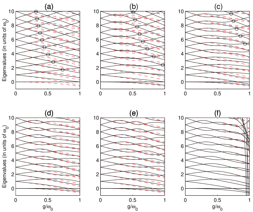
Figure 2: Comparison of the exact numerical eigenvalues (dashed lines) of (8) for one-photon resonance $\omega=\omega_{0}$ with the approximate ones (solid lines) obtained respectively after (a) 1 one-photon RT given by (47), (b) 1 one-photon RT plus 1 two-photon RT given by (IV), (c) 1 one-photon RT plus 2 two-photon RT, (d) 1 one-photon RT plus 3 two-photon RT, (e) 1 one-photon RT plus 4 two-photon RT, (f) 1 one-photon RT plus 4 two-photon RT plus 1 iteration of KAM-type perturbative expansion. The divergence of the KAM transformation observed close to $g/\omega_{0}=1$ in panel (f) is due to the presence of active resonances at larger values of $g$.

Combining the transformations on the different subspaces we can write the transformation that diagonalizes $H_{1}^{\text{eff}}$ in the Fock space as

$$R_{2}=R_{2,\bot}+R_{(0,2,-)}+P_{(0,+)}$$ (88)

At the right hand side of (87), the three matrices have entries that commute with each other so we can diagonalize the sum of them in the atomic Hilbert space (the second step of $\mathcal{R}_{2,\bot}$ ) as if they had scalar entries. The eigenvalues of $R_{2,\bot}^{{\dagger}}H_{1}^{\text{eff}}P_{\bot}R_{2,\bot}$ are thus:

$$E_{1,(n=1,-)}^{\text{eff}} = \omega-g,~{}~{}~{}~{}E_{1,(n=1,+)}^{\text{eff}}=0,~{}~{}~{}~{}E_{1,(n=2,+)}^{\text{eff}}=0,$$

$$E_{1,(n\geq 3,\pm)}^{\text{eff}} = \omega(n-1)+\frac{g}{2}(\sqrt{n-2}-\sqrt{n})\pm\frac{1}{2}\left[\left(-2\omega+g(\sqrt{n-2}+\sqrt{n})\right)^{2}+g^{2}(n-1)\right]^{1/2}.$$ (89)

As it can be seen from (IV) there are two extra zero eigenvalues which have been added by $R_{2,\bot}$ to the spectrum of $H_{1}^{\text{eff}}$.

Figs. (2-a,b) compare respectively the exact spectrum of $H$ calculated numerically with the spectrum of $H_{0}^{\text{eff}}=H_{JC}$ given by (47) and of $H_{1}^{\text{eff}}$ given by (IV),(79). The crossings of the exact spectrum are all among the eigenvalues with different parities. It is found that the spectrum of $H_{0}^{\text{eff}}$ coincides with the exact one only in the range of quite small coupling. The spectrum of $H_{1}^{\text{eff}}$ has been modified with respect to the one of $H_{0}^{\text{eff}}$ by transforming the encircled crossings between eigenvalues with the same parity into avoided crossings in the small $g$ region. This procedure to treat resonances can be iterated to take into account other resonances appearing at larger values of $g$. Figs. (2-a,b,c,d,e) show how the combination of a one-photon RT and consecutive two-photon RTs lift the artificial degeneracies (marked by circles) of the effective Hamiltonians. The successive steps which we have implemented numerically, transform eigenvalue crossings into avoided crossings. We observe that these RTs also produce an improvement of the approximations of the spectrum. Fig. (2-f) shows the effect of a KAM transformation after the fourth two-photon RT which improves quantitatively the result of Fig. (2-e). The divergence of the KAM transformation close to $g=1$ in Fig. (2-e) is due to the presence of active resonances at larger values of $g$.

V effective Hamiltonians in the Strong-Coupling Regime

In this section we use quantum averaging techniques and RT to obtain the effective Hamiltonians of (8) in the strong-coupling regime. We derive a formula that reproduces the spectrum quite accurately in the whole range of $g$ and for all energies. We consider the Hamiltonian (8) in the strong coupling regime $g\gg\omega_{0}>0$ , which suggests to decompose the Hamiltonian $H$ as

$$H = H_{0}+V,$$

$$H_{0} = \omega(N+1/2)\otimes\openone_{2}+g(a+a^{{\dagger}})\otimes\sigma_{x},$$

$$V = \frac{\omega_{0}}{2}\openone\otimes\sigma_{z}.$$ (90)

that can be interpreted as the system of a quantized field plus the coupling term perturbed by the two-level atom. We remark that in this decomposition, $H_{0}$ contains all the unbounded operators of the complete model and that the perturbation $V$ is a bounded operator. In this case $H_{0}(N,a,a^{{\dagger}},\sigma_{z},\sigma_{x};g)$ is integrable since we can explicitly transform it into a form involving a regular function exclusively of the action operators $N,\sigma_{z}$ (given below in Eq. (V)). To transform $H_{0}$ to a function of action operators, first we diagonalize the term $g(a+a^{{\dagger}})\otimes\sigma_{x}$ in the atomic Hilbert space by the transformation (34):

$$T^{{\dagger}}HT=\omega(N+1/2)\otimes\openone_{2}+g(a+a^{{\dagger}})\otimes\sigma_{z}-\frac{\omega_{0}}{2}\openone\otimes\sigma_{x}.$$ (91)

Next we apply a second unitary transformation

$$U=\left(\begin{array}[]{cc}e^{-\frac{g}{\omega}(a^{{\dagger}}-a)}&0\\ 0&e^{\frac{g}{\omega}(a^{{\dagger}}-a)}\\ \end{array}\right),$$ (92)

to transform $\omega(N+1/2)\otimes\openone_{2}+g(a+a^{{\dagger}})\otimes\sigma_{z}$ into a function of only $N,\sigma_{z}$ (in this case only of $N$):

$$H_{1} := U^{{\dagger}}T^{{\dagger}}HTU=\left[\omega(N+1/2)-\frac{g^{2}}{\omega}\right]\otimes\openone_{2}$$ (95)

$$- \frac{\omega_{0}}{2}\left(\begin{array}[]{cc}0&e^{2\frac{g}{\omega}(a^{{\dagger}}-a)}\\ e^{-2\frac{g}{\omega}(a^{{\dagger}}-a)}&0\\ \end{array}\right)$$

where use has been made of the commutation relations among $a$, $a^{{\dagger}}$, $N$ and the Hausdorff formula:

$$e^{B}Ce^{-B}=C+[B,C]+\frac{1}{2!}[B,[B,C]]+\cdots.$$ (96)

We decompose $H_{1}$ as

$$H_{1} = H_{1}^{(0)}+V_{1},$$

$$H_{1}^{(0)} = U^{{\dagger}}T^{{\dagger}}H_{0}TU=\left[\omega(N+1/2)-\frac{g^{2}}{\omega}\right]\otimes\openone_{2},$$

$$V_{1} = -\omega_{0}/2\left(\begin{array}[]{cc}0&e^{2\frac{g}{\omega}(a^{{\dagger}}-a)}\\ e^{-2\frac{g}{\omega}(a^{{\dagger}}-a)}&0\\ \end{array}\right).$$ (99)

The effective Hamiltonian of the system for strong-coupling regime can thus be written as

$$H_{1}^{\text{eff}}=H_{1}^{(0)}+\Pi_{H_{1}^{(0)}}V_{1}$$ (100)

The eigenvalues of $H_{1}^{(0)}$ have a two-fold degeneracy for every value of $n$ as

$$E_{1,(n,\pm)}^{(0)}=\omega(n+1/2)-\frac{g^{2}}{\omega}$$ (101)

The average of $V_{1}$ relative to $H_{1}^{(0)}$ is thus

$$\Pi_{H_{1}^{(0)}}V_{1} = \sum_{n=0}^{\infty}\{|n,+\rangle\langle n,+|V_{1}|n,-\rangle\langle n,-|$$ (102)

$$+ ~{}|n,-\rangle\langle n,-|V_{1}|n,+\rangle\langle n,+|\}$$

$$= -\frac{\omega_{0}}{2}\sum_{n=0}^{\infty}f_{n}|n\rangle\langle n|\otimes\sigma_{x}~{},$$

with

$$f_{n} = \langle n|e^{\frac{-2g}{\omega}(a^{{\dagger}}-a)}|n\rangle=\langle n|e^{\frac{+2g}{\omega}(a^{{\dagger}}-a)}|n\rangle$$ (103)

$$= e^{-2g^{2}/\omega^{2}}\langle n|e^{\frac{-2g}{\omega}a^{{\dagger}}}e^{\frac{+2g}{\omega}a}|n\rangle$$

$$= e^{-2g^{2}/\omega^{2}}\left(\sum_{j=0}^{n}\frac{(-2g/\omega)^{j}}{j!}\sqrt{\frac{n!}{(n-j)!}}\langle n-j|~{}\right)$$

$$\times \left(~{}\sum_{i=0}^{n}\frac{(+2g/\omega)^{i}}{i!}\sqrt{\frac{n!}{(n-i)!}}|n-i\rangle\right)$$

$$= e^{-2g^{2}/\omega^{2}}\sum_{j=0}^{n}\frac{(2g/\omega)^{2j}(-1)^{j}}{(j!)^{2}}\frac{n!}{(n-j)!}$$

$$= e^{-2g^{2}/\omega^{2}}L_{n}\left(\frac{4g^{2}}{\omega^{2}}\right)$$

where the $L_{n}$ are the Laguerre polynomials. We remark that in the limit of large photon number ($n\rightarrow\infty$), $f_{n}$ can be expressed as a zero-order Bessel function $J_{0}(\frac{4g\sqrt{n}}{\omega})$ Cohen-Tannoudji et al. (1992). $H_{1}$ can be reorganized as

$$H_{1} = H_{1}^{\text{eff}}+(V_{1}-\Pi_{H_{1}^{(0)}}V_{1}),$$

$$H_{1}^{\text{eff}} = \left(\omega(N+1/2)-\frac{g^{2}}{\omega}\right)\otimes\openone_{2}-\frac{\omega_{0}}{2}F\otimes\sigma_{x},$$

$$(V_{1}-\Pi_{H_{1}^{(0)}}V_{1}) = -\frac{\omega_{0}}{2}\left(\begin{array}[]{cc}0&G-F\\ G^{{\dagger}}-F&0\\ \end{array}\right),$$ (106)

where

$$G=e^{\frac{+2g}{\omega}(a^{{\dagger}}-a)},~{}~{}~{}~{}F=\sum_{n=0}^{\infty}f_{n}|n\rangle\langle n|.$$ (107)

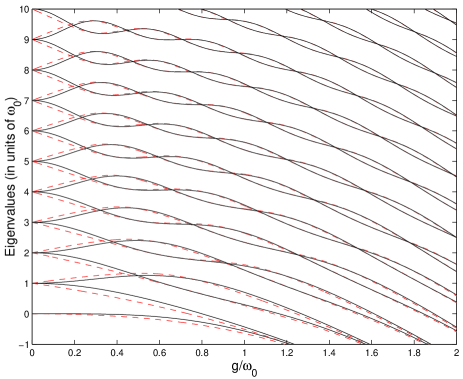
Figure 3: Comparison of exact numerical eigenvalues (dashed lines) of (8) as a function of the coupling constant in the resonant case ($\omega=\omega_{0}$), with the approximate eigenvalues (solid lines) obtained from (113).

$H_{1}^{\text{eff}}$ can easily be diagonalized by applying the transformation (34) that diagonalizes $\sigma_{x}$:

$$H_{2}:=T^{{\dagger}}H_{1}T=H_{2}^{(0)}+V_{2},$$ (108)

with

$$H_{2}^{(0)} = T^{{\dagger}}H_{1}^{\text{eff}}T$$ (109)

$$= \left(\omega(N+1/2)-\frac{g^{2}}{\omega}\right)\otimes\openone_{2}-\frac{\omega_{0}}{2}F\otimes\sigma_{z},$$

and

$$V_{2} = T^{{\dagger}}(V_{1}-\Pi_{H_{1}^{(0)}}{V}_{1})T$$ (112)

$$= -\omega_{0}/4\left(\begin{array}[]{cc}G+G^{{\dagger}}-2F&G-G^{{\dagger}}\\ -G+G^{{\dagger}}&-G-G^{{\dagger}}+2F\\ \end{array}\right).$$

The eigenvalues of $H_{2}^{(0)}$ are therefore

$$E_{2,(n,\pm)}^{(0)}=\omega(n+1/2)-\frac{g^{2}}{\omega}\mp\frac{\omega_{0}}{2}e^{-2g^{2}/\omega^{2}}L_{n}(\frac{4g^{2}}{\omega^{2}}).$$ (113)

which is the same result obtained in Graham and Höhnerbach (1984a); Tur (2000); Franchuk et al. (1996) by other methods. Figure (3) compares the exact numerical spectrum of (8) with the approximation (113) for the resonant case $\omega=\omega_{0}$. One can see that for large enough $g$, the formula (113) reproduces well the spectrum. It is not very accurate for small values of $g$ because of the presence of the one-photon zero-field resonances that we analyze as follows. In the limit $g\rightarrow 0$, we have

$$H_{2}^{(0),g\rightarrow 0} \rightsquigarrow \omega(N+1/2)\otimes\openone_{2}-\frac{\omega}{2}\openone\otimes\sigma_{z},$$

$$V_{2}^{g\rightarrow 0} \rightsquigarrow g\left(\begin{array}[]{cc}0&a-a^{{\dagger}}\\ -(a-a^{{\dagger}})&0\\ \end{array}\right).$$ (116)

Thus degeneracies of $H_{2}^{(0),g\rightarrow 0}$ occur as

$$E_{2,(n,+)}^{(0),g\rightarrow 0}=E_{2,(n-1,-)}^{(0),g\rightarrow 0}.$$ (117)

They are made active by the resonant terms of $V_{2}^{g\rightarrow 0}$:

$$V_{2,res}^{g\rightarrow 0}=\Pi_{H_{2}^{(0)}}^{g\rightarrow 0}V_{2}^{g\rightarrow 0}=-g\left(\begin{array}[]{cc}0&a^{{\dagger}}\\ a&0\\ \end{array}\right).$$ (118)

The transformation (the reduction step of the RT) which transforms this resonant term to a regular function of $N$ is

$$R_{1}:=\left(\begin{array}[]{cc}\openone&0\\ 0&(aa^{{\dagger}})^{-1/2}a\\ \end{array}\right)=\left(\begin{array}[]{cc}\openone{}{}&0\\ 0{}{}&\sum_{n=0}^{\infty}|n\rangle\langle n+1|\\ \end{array}\right),$$ (119)

with the properties

$$R_{1}R^{{\dagger}}_{1}=\openone_{\mathcal{K}},~{}~{}~{}~{}R^{{\dagger}}_{1}R_{1}=\openone_{\mathcal{K}}-\left(\begin{array}[]{cc}0&0\\ 0&|0\rangle\langle 0|\\ \end{array}\right),$$ (120)

We remark that the definition of $R_{1}$ depends on the type of resonant terms. The reduction step of the RT presented here is different from (27). The Hamiltonian transformed under this RT has an extra zero eigenvalue corresponding to spurious eigenvector $|0,-\rangle$, while for the Hamiltonian transformed under (27), the extra zero eigenvalue corresponds to $|0,+\rangle$. Applying $R_{1}$ on $H_{2}$ gives

$$H_{3} := R_{1}^{{\dagger}}H_{2}R_{1}=\left(\omega N-\frac{g^{2}}{\omega}\right)\otimes\openone_{2}+R_{1}^{{\dagger}}V_{2}R_{1}$$ (123)

$$+ \left(\begin{array}[]{cc}\frac{\omega}{2}\left(1-\sum_{n=0}^{\infty}f_{n}|n\rangle\langle n|\right)&0\\ 0&-\frac{\omega}{2}\left(1-\sum_{n=1}^{\infty}f_{n-1}|n\rangle\langle n|\right)-\left(\frac{\omega}{2}+\frac{g^{2}}{\omega}\right)|0\rangle\langle 0|\\ \end{array}\right).$$

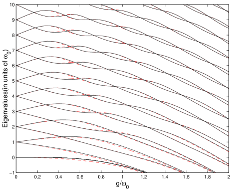
Figure 4: Comparison of exact numerical spectrum of (8) (dashed lines) as a function of the coupling constant in the resonant case ($\omega=\omega_{0}$), with the quite accurate result (V) which has treated the zero-field resonances by a RT (solid lines).

Next, we take $H_{3}^{(0)}=\omega N\otimes\openone_{2}$ and the rest of $H_{3}$ as $V_{3}$. Since $H_{3}^{(0)}$ has a two-fold degeneracy as $E_{3,(n,+)}^{(0)}=E_{3,(n,-)}^{(0)}$, the average of $V_{3}$ relative to $H_{3}^{(0)}$ is thus

$$\Pi_{H_{3}^{(0)}}V_{3}=\left(\begin{array}[]{cc}\frac{\omega}{2}-\frac{g^{2}}{\omega}-\frac{\omega}{2}\sum_{n=0}^{\infty}f_{n}|n\rangle\langle n|&\sum_{n=1}^{\infty}-\frac{g}{\sqrt{n}}e^{-2g^{2}/\omega^{2}}L_{n-1}^{(1)}(\frac{4g^{2}}{\omega^{2}})|n\rangle\langle n|\\ \sum_{n=1}^{\infty}-\frac{g}{\sqrt{n}}e^{-2g^{2}/\omega^{2}}L_{n-1}^{(1)}(\frac{4g^{2}}{\omega^{2}})|n\rangle\langle n|&-(\frac{\omega}{2}+\frac{g^{2}}{\omega})(1-|0\rangle\langle 0|)+\frac{\omega}{2}\sum_{n=1}^{\infty}f_{n-1}|n\rangle\langle n|\\ \end{array}\right),$$ (124)

where we have used the relation Frasca (2002)

$$\langle m|e^{\pm\frac{2g}{\omega}(a^{{\dagger}}-a)}|n\rangle=\sqrt{\frac{n!}{m!}}\left(\frac{\pm 2g}{\omega}\right)^{m-n}e^{-\frac{2g^{2}}{\omega^{2}}}L_{n}^{(m-n)}\left(\frac{4g^{2}}{\omega^{2}}\right),$$ (125)

with $L_{n}^{(m-n)}(x)$ the associated Laguerre polynomials. The new effective Hamiltonian can thus be written as

$$H_{3}^{\text{eff}}=\omega N\otimes\openone_{2}+\Pi_{H_{3}^{(0)}}V_{3}.$$ (126)

Since all the entries of $H_{3}^{\text{eff}}$ commute with $N$, it can be diagonalized in the atomic Hilbert space as if its entries were scalars. The eigenvalues of $H_{3}^{\text{eff}}$ are thus

$$E_{3,(0,-)}^{\text{eff}} = 0,~{}~{}~{}~{}~{}~{}~{}~{}~{}~{}~{}~{}E_{3,(0,+)}^{\text{eff}}=\frac{\omega}{2}-\frac{g^{2}}{\omega}-\frac{\omega}{2}e^{\frac{-2g^{2}}{\omega^{2}}},$$

$$E_{3,(n\geq 1,\pm)}^{\text{eff}} = n\omega-\frac{g^{2}}{\omega}-\frac{\omega}{4}e^{\frac{-2g^{2}}{\omega^{2}}}\left(L_{n}(\frac{4g^{2}}{\omega^{2}})-L_{n-1}(\frac{4g^{2}}{\omega^{2}})\right)$$ (127)

$$\pm \frac{1}{2}\left[\left(\omega-\frac{\omega}{2}e^{\frac{-2g^{2}}{\omega^{2}}}\left(L_{n}(\frac{4g^{2}}{\omega^{2}})+L_{n-1}(\frac{4g^{2}}{\omega^{2}})\right)\right)^{2}+\frac{4g^{2}}{n}e^{\frac{-4g^{2}}{\omega^{2}}}\left(L_{n-1}^{(1)}(\frac{4g^{2}}{\omega^{2}})\right)^{2}\right]^{1/2}.$$

The zero eigenvalue is the extra spurious one that has been added by the RT to the spectrum. Fig. (4) compares the exact numerical spectrum of (8) and the approximation (V) which has treated the zero-field resonances by a RT. The figure shows that treating all the active resonances of the system allows to obtain all the qualitative features of the spectrum in the whole range of the coupling constant and for all energies. At a second stage, since we have treated all the active resonances, we can improve further this spectrum quantitatively by a KAM-type perturbative iteration.

VI Conclusions

We have presented a non-perturbative method based on the quantum averaging technique to determine the spectral properties of systems containing resonances. It consists in the construction of unitary or isometric transformations that leads to an effective reduced Hamiltonian. These transformations are composed of two qualitatively distinct stages. The first one consists of non-perturbative transformations (RTs) that are adapted to the structure of the resonances. Their role is to construct a first effective Hamiltonian that contains the main qualitative features of the spectrum – crossings and avoided crossings – in a given range of the coupling parameter. The diagonalized form of this effective Hamiltonian, which depends parametrically on the coupling constant, is then taken as a new reference Hamiltonian around which one can apply perturbative techniques to improve the quantitative accuracy of the spectrum. We formulate the perturbative approach in terms of a KAM-type iteration of contact transformations. Similar results can be obtained with other formulations of perturbation theory.

We have illustrated the method with a model of a two level atom interacting with a single mode of a quantized field. The method can be applied to more general systems with several field modes. It can also be adapted to the treatment of semi-classical models in which the field is described as a time-dependent function.

We have analyzed the resonances in two regimes of weak and strong coupling. The results we obtained in the weak-coupling regime can be expected to be applicable to quite general models. The analysis of the strong-coupling regime of this model leads to results that are valid for all values of the coupling and for all energies. The possibility to obtain such a global result is due to a particular property of the model, and one cannot expect to obtain it for general models. The particular property is that the part we selected as the reference Hamiltonian $H_{0}$ in the strong-coupling regime contains all the unbounded operators of the complete model and is explicitly solvable. The term that was left to be treated by RT and perturbation theory is a bounded operator.

References

Jaynes and Cummings (1963)
E. Jaynes and
F. Cummings,
Proc. IEEE 51,
89 (1963).
Shirley (1965)
J. Shirley,
Phys. Rev. 138,
979 (1965).
Jauslin et al. (2000)
H. R. Jauslin,
S. Guérin,
and S. Thomas,
Physica A 279,
432 (2000).
Guérin and Jauslin (2003)
S. Guérin and
H. R. Jauslin,
Adv. Chem. Phys. 125,
147 (2003).
Bellissard (1985)
J. Bellissard, in
Trends and Developments in the Eighties, edited
by S. Albeverio
and P. Blanchard
(World Scientific, Singapore,
1985).
Primas (1963)
H. Primas,
Rev. Mod. Phys. 35,
710 (1963).
Milonni et al. (1983)
P. W. Milonni,
J. R. Ackerhalt,
and H. W.
Galbraith, Phys. Rev. Lett.
50, 966 (1983).
Allen and Eberly (1975)
L. Allen and
J. H. Eberly,
Optical resonance and two-level atoms
(Wiley, New York,
1975).
Lais and Steimle (1990)
P. Lais and
T. Steimle,
Opt. Commun. 78,
346 (1990).
Cohen-Tannoudji
et al. (1992)
C. Cohen-Tannoudji,
J. Dupont-Roc,
and G. Grynberg,
Atom-Photon Interactions (Wiley,
New York, 1992),
chap. 6, pp. 408,485.
Frasca (2002)
M. Frasca,
Phys. Rev. A 66,
023810 (2002).
Graham and
Höhnerbach (1984a)
R. Graham and
M. Höhnerbach,
Z. Phys. B 57,
233 (1984a).
Graham and
Höhnerbach (1984b)
R. Graham and
M. Höhnerbach,
Phys. Lett.A 101,
61 (1984b).
Franchuk et al. (1996)
I. Franchuk,
L. Komarov, and
A. Ulyanenkov,
J. Phys. A 29,
4035 (1996).
Tur (2000)
E. Tur, Opt.
Spec. 89, 574
(2000).
Weigert and Müller (1995)
S. Weigert and
G. Müller,
Chaos, Solitons and Fractals 5,
1419 (1995).
Reed and Simon (1980)
M. Reed and
B. Simon,
Methods of Modern Mathematical Physics: Functional
Analysis, vol. 1 (Academic,
London, 1980).
Bérubé-Lauzière
et al. (1994)
Y. Bérubé-Lauzière,
V. Hussin, and
L. Nieto,
Phys. Rev. A 50,
1725 (1994).