Designing robust gate implementations for quantum information processing

Abstract

Quantum information processing systems are often operated through time dependent controls; choosing these controls in a way that makes the resulting operation insensitive to variations in unknown or uncontrollable system parameters is an important prerequisite for obtaining high-fidelity gate operations. In this article we present a numerical method for constructing such robust control sequences for a quite general class of quantum information processing systems. As an application of the method we have designed a robust implementation of a phase-shift operation central to rare earth quantum computing, an ensemble quantum computing system proposed by Ohlsson et. al. Ohlsson et al. (2002). In this case the method has been used to obtain a high degree of insensitivity with respect to differences between ensemble members, but it is equally well suited for quantum computing with a single physical system.

Introduction

Many potential quantum information processing systems are controlled by means of a set of time-dependent parameters, such as quasi-static electromagnetic fields Nakamura et al. (1999), radio-frequency, Cory et al. (1997); Kane (1998), or optical fields Cirac and Zoller (1995); Imamoglu et al. (1999); Lukin and Hemmer (2000); Ohlsson et al. (2002). For most such systems, it is relatively simple to device a set of controls that implement a given evolution in an ideal situation. Often, however, a more careful choice of controls can lead to an implementation that is less sensitive to variations in unknown or uncontrollable system parameters. Examples of such robust implementations include system specific solutions such as the hot gate for ion trap quantum computing which is insensitive to vibrational excitations Sørensen and Mølmer (1999), as well as more general techniques such as composite pulses, a technique originating in NMR spectroscopy Cummins et al. (2003).

In this article we describe a numerical method for designing robust controls for systems where the evolution is adequately described by a possibly non-unitary evolution operator $\mathbf{U}(t)$. This form does not allow a general master equation formulation, but it is sufficient to establish worst case behavior in many quantum computing settings where the worst case effects of decoherence and loss can be adequately modeled by a Schrödinger equation with a non-Hermitian Hamiltonian.

As an application of the method, we will consider the construction of a robust phase shift operation for the rare earth quantum computing (REQC) system Ohlsson et al. (2002); Longdell and Sellars (2002), which is based on rare-earth ions embedded in a cryogenic crystal. In each ion, two metastable ground-state hyperfine levels, labeled $\left\lvert{0}\right\rangle$ and $\left\lvert{1}\right\rangle$, serve as a qubit register which is manipulated via optical transitions from both states to an inhomogeneously shifted excited state $\left\lvert{\text{e}}\right\rangle$. The REQC system is an ensemble quantum computing system and macroscopic numbers of ions are manipulated in parallel, addressed by the value of the inhomogeneous shift of their $\left\lvert{\text{e}}\right\rangle$-state. To obtain a sufficient number of ions within each frequency channel, it is necessary to operate on all ions within a finite range of inhomogeneous shifts, and the main difficulty in operating the REQC system is to achieve the same evolution for each of these ions independent of their particular inhomogeneous shift.

This article is divided into two sections: in section I we describe the method we have used to design robust gate implementations; these results should be applicable to a variety of quantum information processing systems. In section II we present the results of applying the method to a specific problem relating to the REQC system, and show that it is indeed possible to obtain very high degrees of robustness.

I Designing robust gate implementations

We consider a collection of quantum system which evolve according to a set of time-dependent controls $\boldsymbol{\varepsilon}(t)$. In addition to $\boldsymbol{\varepsilon}$, the single system Hamiltonian $H(\boldsymbol{\xi},\boldsymbol{\varepsilon}(t))$ depends on a system specific set of uncontrollable or unknown parameters $\boldsymbol{\xi}$, such as field strength or quantum numbers corresponding to unused degrees of freedom.

The evolution of each system is governed by the Schrödinger equation,

$$i\hbar\frac{\partial}{\partial{t}}\mathbf{{U}}(t)=H(\boldsymbol{\xi},\boldsymbol{\varepsilon}(t))\,\mathbf{{U}}(t),\qquad\mathbf{{U}}(0)=\boldsymbol{1},$$ (1)

where we will allow the Hamiltonian $H$ to include non-Hermitian terms describing loss and decoherence.

Our goal is to choose a set of controls that lead to an evolution $\mathbf{U}(T)$ which is as close as possible to a given desired evolution $\mathbf{U}_{0}$ over a range of $\boldsymbol{\xi}$-values. To quantify this, we introduce an objective functional $J(\boldsymbol{\xi},\boldsymbol{\varepsilon})$ which describes the performance of a set of controls $\boldsymbol{\varepsilon}$ for a given value of $\boldsymbol{\xi}$. By convention we take a low value of $J$ to indicate a good performance, and the problem of finding a robust set of controls thus corresponds to minimizing

$$J_{X}(\boldsymbol{\varepsilon})=\max_{\boldsymbol{\xi}\in X}J(\boldsymbol{\xi},\boldsymbol{\varepsilon}),$$ (2)

where $X$ is the set of $\boldsymbol{\xi}$-values for which we want the implementation to perform well. The conceptually simple approach we have taken to this problem is to replace $X$ with a discrete subset $X^{\prime}\subset X$, so that the minimization of $J_{X^{\prime}}$ has the form of a standard minimax problem, which can be solved efficiently provided that we are able to calculate $\partial J_{X^{\prime}}/\partial\boldsymbol{\varepsilon}$. Below we show how to achieve this by methods from optimal control theory.

I.1 Calculating $\partial J/\partial\boldsymbol{\varepsilon}$

In this section we show how $\partial J/\partial\boldsymbol{\varepsilon}$ may be calculated for a quite general class of objective functionals. To keep the notation simple and avoid unnecessary restrictions, we will consider the following generalization of the Schrödinger equation (1),

$$\dot{\mathbf{{U}}}(t)=\boldsymbol{f}(\mathbf{{U}}(t),\boldsymbol{\varepsilon}(t)),\qquad\mathbf{{U}}(0)=\boldsymbol{1},$$ (3)

determining the evolution of a complex-valued, time-dependent matrix $\mathbf{{U}}$ due to a set of real-valued, time-dependent controls, $\boldsymbol{\varepsilon}(t)$. We will consider objective functionals of the form

$$J(\boldsymbol{\varepsilon})=\phi(\mathbf{{U}}(T))+\int_{0}^{T}l(\mathbf{{U}}(t),\boldsymbol{\varepsilon}(t))dt,$$ (4)

where $\phi(\mathbf{{U}}(T))$ is a real-valued function quantifying how close the final state $\mathbf{U}(T)$ is to our goal, and the real valued function $l((\mathbf{{U}}(t),\boldsymbol{\varepsilon}(t))$, referred to as a penalty function, can be chosen to discourage the use of certain control values. Our goal is to calculate $\partial J/\partial\boldsymbol{\varepsilon}$ subject to the constraint that $\boldsymbol{\varepsilon}$ and $\mathbf{{U}}$ obey Eq. (3). To achieve this we introduce the modified objective functional:

$$J^{\prime}=J-\int_{0}^{T}\operatorname*{Tr}\left(\mathbf{{\Lambda}}^{\dagger}\left[\dot{\mathbf{{U}}}-\boldsymbol{f}(\mathbf{{U}},\boldsymbol{\varepsilon})\right]+\text{h.c.}\right)dt,$$ (5)

where the complex time-dependent adjoint state matrix $\mathbf{{\Lambda}}$ is in effect a continuous set of Lagrange multipliers leaving $J^{\prime}$ identical to $J$, provided that $\mathbf{{U}}$ and $\boldsymbol{\varepsilon}$ obey Eq. (3). If we require $\mathbf{{\Lambda}}$ to obey the adjoint equations

$$\dot{\mathbf{{\Lambda}}}^{\dagger}=-\frac{\partial{h}}{\partial\mathbf{{U}}},\qquad\mathbf{{\Lambda}}^{\dagger}(T)=\left.{\frac{\partial\phi}{\partial\mathbf{{U}}}}\right\rvert_{T},$$ (6)

where $\mathbf{{U}}$ and $\mathbf{{U}}^{\dagger}$ should be considered as independent with respect to the partial derivative and $h$ is defined as

$$h(\boldsymbol{\varepsilon},\mathbf{{U}},\mathbf{{\Lambda}})=l(\mathbf{{U}},\boldsymbol{\varepsilon})+\operatorname*{Tr}\left(\mathbf{{\Lambda}}^{\dagger}\boldsymbol{f}(\mathbf{{U}},\boldsymbol{\varepsilon})+\text{h.c.}\right),$$ (7)

we find by integration by parts that the differential of $J^{\prime}$ is given by Luenberger (1979)

$$dJ^{\prime}=\int_{0}^{T}\frac{\partial h}{\partial\boldsymbol{\varepsilon}}\;\delta\boldsymbol{\varepsilon}(t)\,dt,$$ (8)

from which the derivatives of $J$ with respect to the parameters used to parametrize $\boldsymbol{\varepsilon}$ can be calculated by the chain rule.

We now return to the case of a quantum system governed by the Schrödinger equation (1). If we assume the penalty function $l$ to be independent of $\mathbf{{U}}$, the adjoint equations in this case are

$$i\hbar\frac{\partial}{\partial{t}}\mathbf{{\Lambda}}(t)=H^{\dagger}(\boldsymbol{\xi},\boldsymbol{\varepsilon}(t))\,\mathbf{{\Lambda}}(t),\qquad\mathbf{{\Lambda}}(T)=\left.{\frac{\partial\phi}{\partial\mathbf{{U}}^{\dagger}}}\right\rvert_{T},$$ (9)

and $dJ$ is given by (8) with

$$\frac{\partial h}{\partial\boldsymbol{\varepsilon}}=\frac{\partial l}{\partial\boldsymbol{\varepsilon}}+\frac{2}{\hbar}\operatorname*{Im}\operatorname*{Tr}\left(\mathbf{{\Lambda}}^{\dagger}\frac{\partial H}{\partial\boldsymbol{\varepsilon}}\mathbf{{U}}\right).$$ (10)

The role of the adjoint state and the adjoint equations is often described as back-propagating the errors in achieving the desired final state. If $H$ is Hermitian, the boundary value for $\mathbf{{\Lambda}}$ can be optimized for numerical computation as shown in Appendix B.

I.2 Fidelity of quantum evolution

We will now discuss the choice of the function $\phi$, quantifying how well the obtained evolution $\mathbf{U}(T)$ approximates $\mathbf{U}_{0}$. As we are concerned with quantum information processing we will assume that all operations start out with an unknown state in the qubit subspace $\mathcal{H}_{Q}$ of the full system Hilbert space $\mathcal{H}$, and that this subspace is invariant under the ideal evolution $\mathbf{U}_{0}$. The function $\phi$ should not depend on the evolution of states outside $\mathcal{H}_{Q}$, nor on collective phases on the states originating in $\mathcal{H}_{Q}$. A cautious choice of $\phi$ fulfilling these conditions could be based on the worst case overlap fidelity Nielsen and Chuang (2000):

$$\mathcal{F}=\min_{\left\lvert{\psi}\right\rangle\in\mathcal{H}_{Q}}\left|\left<{\psi}\,\vrule\,{\mathbf{U}_{0}^{\dagger}\mathbf{U}(T)}\,\vrule\,{\psi}\right>\right|,$$ (11)

which measures the least possible overlap between the obtained output state $\mathbf{U}(T)\left\lvert{\psi}\right\rangle$ and the ideal output $\mathbf{U}_{0}\left\lvert{\psi}\right\rangle$ for initial states in $\mathcal{H}_{Q}$. This fidelity measure has the desirable quality that both population transfer from $\mathcal{H}_{Q}$ to $\mathcal{H}_{Q}^{\perp}$ and population transfer completely out of $\mathcal{H}$, as described by a non-unitary evolution, is counted as loss of fidelity.

From the point of view of optimal control, a significant drawback of the worst case overlap fidelity, $\mathcal{F}$, is that it is computationally complicated Wesenberg and Mølmer (2003). A computationally accessible fidelity measure which share many appealing features with $\mathcal{F}$ is the trace fidelity Palao and Kosloff (2002),

$$\mathcal{T}=\frac{1}{n}\left|\operatorname*{Tr}_{\mathcal{H}_{Q}}\left(\mathbf{U}_{0}^{\dagger}\,\mathbf{U}\right)\right|,$$ (12)

where $n=\dim(\mathcal{H}_{Q})$. As shown in Appendix A, $\mathcal{T}$ is related to $\mathcal{F}$ by the strict bound

$$1-\mathcal{F}\leq n(1-\mathcal{T}),$$ (13)

indicating that we can safely replace $\mathcal{F}$ by $\mathcal{T}$ for numerical computations on a few qubits at high fidelity.

For numerical calculations it is beneficial to use $\mathcal{T}^{2}$ rather than $\mathcal{T}$ Palao and Kosloff (2003); in the calculations presented in the next section we have used $\phi=1-\mathcal{T}^{2}$, leading to an adjoint state boundary condition of

$$\mathbf{{\Lambda}}(T)=\left.{\frac{\partial\phi}{\partial\mathbf{{U}}^{\dagger}}}\right\rvert_{T}\,=-\frac{1}{n^{2}}\mathbf{{U}}_{0}\;\operatorname*{Tr}(\mathbf{{U}}_{0}^{\dagger}\mathbf{{U}}(T)),$$ (14)

which can be directly computed.

I.3 Minimization algorithms

One approach to minimizing $J$ is to directly solve the extremum condition $\partial J/\partial\boldsymbol{\varepsilon}=0$ for $\boldsymbol{\varepsilon}$. This task is significantly simplified if a penalty function proportional to $\boldsymbol{\varepsilon}^{2}$ is introduced, $h=\lambda\boldsymbol{\varepsilon}^{2}+h_{0}$, so that the extremum condition according to (8) reads,

$$\boldsymbol{\varepsilon}(t)=-\frac{1}{2\lambda}\frac{\partial h_{0}}{\partial\boldsymbol{\varepsilon}},$$ (15)

which may be used as an iterative formula for calculating $\boldsymbol{\varepsilon}$. Variations over this iterative approach give rise to the Krotov Tannor et al. (1992) and Zhu-Rabitz Zhu and Rabitz (1998a, b) algorithms which have been shown to have excellent convergence properties, and have been successfully applied to optimal control of unitary transformations for one set of parameters by the group of R. Kosloff Palao and Kosloff (2003, 2002). A unifying view of these direct methods can be found in Ref. Maday and Turinici (2003).

In the work presented here we have chosen to use an indirect minimization algorithm: rather than trying to solve the extremum condition directly, we have used the gradient information obtained through Eq. (8) as input for a general sequential quadratic programming procedure based on a constrained quasi-Newton method Fletcher (1987); Gill et al. (1981); Lin and Moré (1999). The primary advantage of this approach is that we have total freedom to choose the parametrization of the controls, and can place arbitrary bounds on these. This allows us to more accurately model the fact that the experimental limitations most often only distinguish between possible and impossible controls: no possible controls are significantly harder than others. An explicit field strength limit also serves to introduce an absolute scale on which to introduce decay strengths etc.

II Application to rare earth quantum computing

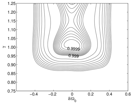
(a) $\operatorname{sech}$-pulses

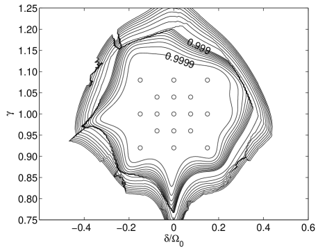
(b) Optimized pulse

Figure 1: The worst case overlap fidelity of $\mathbf{U}_{0}$ as given by Eq. (16) implemented (a) by a series of $\operatorname{sech}$ pulses as suggested by Roos and Mølmer Roos and Mølmer (2003), and (b) by an optimized pulse. The fidelity is plotted as a function of relative field strength $\gamma$ and inhomogeneous shift $\delta$ relative to the maximal resonant Rabi frequency $\Omega_{0}$. The duration of both pulses is $24\pi/\Omega_{0}$, and the circles in (b) indicates the parameter set $X^{\prime}$ used during the optimization.

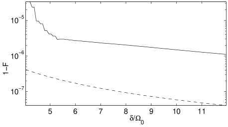
Figure 2: The effect of the $\operatorname{sech}$-pulse sequence (dashed line) and the optimized (solid line) implementation of $\mathbf{U}_{0}$ on far-detuned ions, as described by $1-\mathcal{F}$, where $\mathcal{F}$ is calculated with respect to the identity, as these ions should ideally not be disturbed. Both implementations achieve worst case fidelities very close to unity, with the $\operatorname{sech}$-pulse sequence achieving the best results. The curve for the optimized pulse is actually a running maximum, as the actual value of $1-\mathcal{F}$ oscillates with a period of $2\pi/T$.

The motivation for the work presented in this article has been the design of robust gate implementations for the REQC system mentioned in the introduction. As an example, we will consider the construction of a robust implementation of the single qubit operation

$$\mathbf{U}_{0}=\left\lvert{1}\right\rangle\left\langle{1}\right\rvert-\left\lvert{0}\right\rangle\left\langle{0}\right\rvert,$$ (16)

which could simply be implemented by a single $2\pi$ pulse on the $\left\lvert{0}\right\rangle$-$\left\lvert{\text{e}}\right\rangle$ transition if we were not concerned with robustness. Our primary concern will be to make the implementation robust with respect to variations in the inhomogeneous shift $\delta$ of the $\left\lvert{\text{e}}\right\rangle$-state in order to allow the use of finite with channels. Since it is experimentally difficult to obtain a homogeneous field strength over the crystal, we would also prefer the implementation to be insensitive to variations in the relative field strength, which we will denote $\gamma$.

In addition to requiring the implementation of $\mathbf{U}_{0}$ to be robust with respect to variations in $\delta$ and $\gamma$, we will add the requirement that ions outside the channels should not be affected, as this allows us to use the obtained implementation of $\mathbf{U}_{0}$ as a part of a controlled phase shift operation Lukin and Hemmer (2000); Ohlsson et al. (2002): If the $\left\lvert{\text{e}}\right\rangle$-states of the qubit ion and a controlling ion are coupled sufficiently strongly by static dipole interaction, an excitation of the controlling ion will effectively shift the qubit ion out of the channel thus conditioning the evolution of the qubit on the state of the controlling ion.

Even though the simplest implementation of $\mathbf{U}_{0}$ for an ideal ion with $\delta=0$ and $\gamma=1$ would involve only the $\left\lvert{0}\right\rangle$ and $\left\lvert{\text{e}}\right\rangle$ levels, a robust implementation must also involve the $\left\lvert{1}\right\rangle$-state since the coupling of $\left\lvert{0}\right\rangle$ to $\left\lvert{\text{e}}\right\rangle$ will result in a $\delta$-dependent phase on $\left\lvert{0}\right\rangle$ which can only be compensated by introducing the same phase on the $\left\lvert{1}\right\rangle$-state, e.g. through phase compensating rotations Wesenberg and Mølmer (2003). A highly successful example of this approach is the $\operatorname{sech}$-pulse sequence suggested by Roos and Mølmer Roos and Mølmer (2003), which as illustrated by Fig. 1(a) yields a very robust implementation, achieving high fidelities over a wide range of parameter values.

We model the REQC system by the single ion Hamiltonian

$$H=-\delta\left\lvert{\text{e}}\right\rangle\left\langle{\text{e}}\right\rvert+\frac{\gamma}{2}\sum_{i=0,1}\left(\Omega_{i}(t)\left\lvert{\text{e}}\right\rangle\left\langle{i}\right\rvert+\text{h.c.}\right),$$ (17)

which does not include any effects of decay or decoherence. In the notation introduced in section I, the system parameters are $\boldsymbol{\xi}=(\gamma,\delta)$, the controls are $\boldsymbol{\varepsilon}=(\Omega_{0},\Omega_{1})$, and the qubit subspace is $\mathcal{H}_{Q}=\{\left\lvert{0}\right\rangle,\left\lvert{1}\right\rangle\}$. No penalty function is used: we use $J=\phi=1-\mathcal{T}^{2}$, and limit the field by strict bounds on $\Omega_{i}(t)$, as this is the relevant limiting parameter in the REQC system. Inspired by the success of the $\operatorname{sech}$-based solution and the hat-like Fourier spectrum of the $\operatorname{sech}$-pulse, $\Omega_{i}(t)$ is parametrized in terms of a truncated Fourier basis. Based on trial and error we have arrived at $49$ $\boldsymbol{\xi}$-values to constitute $X^{\prime}$, some within the neighborhood of $\delta=0$, $\gamma=1$, and some at large detunings where the ions should not be disturbed. The result of the optimization with this choice of $X^{\prime}$ is shown in Fig. 1(b), where the circles indicate the members of $X^{\prime}$. It is evident from the plot that the optimization has achieved a high fidelity over an even larger range of parameters than the $\operatorname{sech}$-pulse sequence illustrated in Fig. 1(a).

With respect to not disturbing the detuned ions, both the optimized pulse and the $\operatorname{sech}$-pulses obtain fidelities within $10^{-5}$ of unity for $|\delta|>5\Omega_{0}$, where $\Omega_{0}$ is the maximal resonant Rabi frequency at $\gamma=1$. As illustrated by Fig. 2, which only shows fidelities at $\gamma=1$ as $\mathbf{U}(T)$ is nearly independent of $\gamma$ at $|\delta|\gg\Omega_{0}$, the $\operatorname{sech}$-pulse sequence performs better than the optimized pulse in this regime.

III Conclusions and outlook

We have shown that it is possible to construct highly robust gate implementations for quantum information processing by a quite general method. In particular, the method has been used to greatly enhance the performance of a gate implementation for a model REQC system by extending the range of inhomogeneous shifts and relative field strengths over which an acceptable performance is achieved.

The model REQC system used in this article ignores many performance degrading factors, the two most important being decoherence and implementation noise. Decoherence could in the present case be adequately modeled by a non-Hermitian Hamiltonian, for which we expect the method described in this paper to be able to find a robust implementation as in the decoherence-free case. It is not clear, however, how the method could be extended to address the problem of robustness with respect to implementation imperfections.

Appendix A The trace fidelity

In this section we prove the relation (13) between the worst case overlap fidelity, $\mathcal{F}$, and the trace fidelity $\mathcal{T}$. Referring to the definition (11), we note that $\mathcal{F}$ is completely determined by the restriction $\mathbf{{O}}$ of the operator $\mathbf{U}_{0}^{\dagger}\mathbf{U}(T)$ to $\mathcal{H}_{Q}$. Since $\mathbf{U}(T)$ describes the evolution of a quantum system, it is possible to extend it to a unitary operation on a Hilbert space containing $\mathcal{H}$, and $\mathbf{{O}}$ is consequently the restriction of a unitary operator to $\mathcal{H}_{Q}$. In the ideal case $\mathbf{{O}}$ will be equal to the identity on $\mathcal{H}_{Q}$, perhaps with the exception of a complex phase.

$\mathcal{F}$ is defined as the minimum of the overlap $|\left<{\psi}\,\vrule\,{\mathbf{{O}}}\,\vrule\,{\psi}\right>|$. Since the unit sphere of $\mathbb{C}^{n}$ is compact, this minimum will be attained for some $\left\lvert{\psi_{0}}\right\rangle$: $\mathcal{F}=|\left<{\psi_{0}}\,\vrule\,{\mathbf{{O}}}\,\vrule\,{\psi_{0}}\right>|$. We now extend $\{\left\lvert{\psi_{0}}\right\rangle\}$ to an orthonormal basis $\{\left\lvert{\psi_{k}}\right\rangle\}_{k=0,\ldots,n-1}$ by the Gram-Schmidt process. Evaluating the trace fidelity in this basis we find by the triangle inequality:

$$\mathcal{T} \leq\frac{1}{n}\sum_{k=0}^{n-1}\left|\left<{\psi_{k}}\,\vrule\,{\mathbf{{O}}}\,\vrule\,{\psi_{k}}\right>\right|$$ (18a)

$$\leq\frac{1}{n}\left(\mathcal{F}+(n-1)\right),$$ (18b)

where we have used that $|\left<{\psi}\,\vrule\,{\mathbf{{O}}}\,\vrule\,{\psi}\right>|\leq 1$ for all $\left\lvert{\psi}\right\rangle$ since $\mathbf{{O}}$ is the restriction of a unitary operator. By rewriting (18b) we obtain the desired relation, $1-\mathcal{F}\leq n(1-\mathcal{T})$.

We note that the established bound is strict in the sense that for any $0\leq\mathcal{F}_{0}\leq 1$, the operator

$$\mathbf{{O}}_{\mathcal{F}}=\boldsymbol{1}-(1-\mathcal{F}_{0})\left\lvert{\psi}\right\rangle\left\langle{\psi}\right\rvert$$ (19)

will fulfill Eq. (13) with equality for any $\left\lvert{\psi}\right\rangle$.

Appendix B Optimized adjoint state boundary condition

In the case of a Hermitian Hamiltonian and a penalty function $l$, that does not depend on the state $\mathbf{{U}}$, it is possible to modify the adjoint state boundary condition (14) to reduce the required accuracy of the adjoint state propagation.

In this case, we find according to Eqs. (8) and (10) that $dJ$ has the form

$$dJ=\int_{0}^{T}\left[\frac{\partial l}{\partial\boldsymbol{\varepsilon}}+2\operatorname*{Im}\left(\sum_{k}\boldsymbol{\lambda}_{k}^{\dagger}\frac{\partial H}{\partial\boldsymbol{\varepsilon}}\boldsymbol{x}_{k}\right)\right]\delta\boldsymbol{\varepsilon}(t)\,dt,$$ (20)

where $\boldsymbol{x}_{k}$ and $\boldsymbol{\lambda}_{k}$ denotes the $k$-th columns of $\mathbf{{U}}$ and $\mathbf{{\Lambda}}$ respectively. Since $H$ and thus $\partial H/\partial\boldsymbol{\varepsilon}$ are assumed to be Hermitian, $dJ$ as given by (20) is not affected by adding to $\boldsymbol{\lambda}_{k}$ a component of $\alpha_{k}\boldsymbol{x}_{k}$ for any real $\alpha_{k}$. Furthermore, since $\boldsymbol{\lambda}_{k}$ and $\boldsymbol{x}_{k}$ evolve according to the same Schrödinger equation, this corresponds to modifying the boundary condition for the adjoint state to read:

$$\boldsymbol{\lambda}_{k}(T)=\frac{\partial\phi}{\partial\boldsymbol{x}_{k}^{\dagger}}+\alpha_{k}\boldsymbol{x}_{k}(T),$$ (21)

for any real $\alpha_{k}$.

The obvious use of the freedom in the choice of boundary value is to minimize the norm of the adjoint state, in order to relax the requirements of the relative precision of the adjoint state propagation. This minimum is easily calculated from (21), but we prefer to illustrate the physical background of the result by calculating it in a different way: The freedom in the choice of boundary value (21) is allowed by the Hermiticity of $H$. The same Hermiticity ensures that $\boldsymbol{x}_{k}$ is normalized, so that $\phi\circ\boldsymbol{n}(\boldsymbol{x}_{k})$, where $\boldsymbol{n}$ is the normalization function $\boldsymbol{n}(\boldsymbol{v})=\boldsymbol{v}/|\boldsymbol{v}|$, is equal to $\phi(\boldsymbol{x}_{k})$. The gradient of $\tilde{\phi}=\phi\circ\boldsymbol{n}$, however, is different from that of $\phi$. In fact we find

$$\frac{\partial\tilde{\phi}}{\partial\boldsymbol{x}_{k}^{\dagger}}=\frac{\partial\phi}{\partial\boldsymbol{x}_{k}^{\dagger}}-\operatorname*{Re}\left[\boldsymbol{x}_{k}^{\dagger}\frac{\partial\phi}{\partial\boldsymbol{x}_{k}^{\dagger}}\right]\;\boldsymbol{x}_{k},$$ (22)

where $\boldsymbol{x}_{k}$ and $\boldsymbol{x}_{k}^{\dagger}$ should be considered independent with respect to the derivative. Comparing this expression to Eq. (21), it is tempting to let $\left.{\alpha_{k}=\operatorname*{Re}(\boldsymbol{x}_{k}^{\dagger}\partial\phi/\partial\boldsymbol{x}_{k}^{\dagger})}\right\rvert_{T}$, which is indeed the answer found by minimizing $|\boldsymbol{x}_{k}(T)|$ subject to Eq. (21).

The modified boundary condition of Eq. (22) carries the same error information as that of Eq. (14), but the required relative numerical precision when propagating the adjoint state will be significantly reduced.

References

- Ohlsson et al. (2002) N. Ohlsson, R. K. Mohan, and S. Kröll, Opt. Comm. 201, 71 (2002).
- Nakamura et al. (1999) Y. Nakamura, Y. A. Pashkin, and J. S. Tsai, Nature 398, 786 (1999).
- Cory et al. (1997) D. G. Cory, A. F. Fahmy, and T. F. Havel, Proc. Natl. Acad. Sci. 94, 1634 (1997).
- Kane (1998) B. E. Kane, Nature 393, 133 (1998).
- Cirac and Zoller (1995) J. I. Cirac and P. Zoller, Phys. Rev. Lett. 74, 4091 (1995).
- Imamoglu et al. (1999) A. Imamoglu, D. D. Awschalom, G. Burkard, D. P. Di-Vincenzo, D. Loss, M. Sherwin, and A. Small, Phys. Rev. Lett. 83, 4204 (1999).
- Lukin and Hemmer (2000) M. D. Lukin and P. R. Hemmer, Phys. Rev. Lett. 84, 2818 (2000).
- Sørensen and Mølmer (1999) A. Sørensen and K. Mølmer, Phys. Rev. Lett. 82, 1971 (1999).
- Cummins et al. (2003) H. K. Cummins, G. Llewellyn, and J. A. Jones, Phys. Rev. A 67 (2003).
- Longdell and Sellars (2002) J. J. Longdell and M. J. Sellars (2002), eprint quant-ph/0208182.
- Luenberger (1979) D. G. Luenberger, Introduction to Dynamic Systems (John Wiley & Sons, 1979).
- Nielsen and Chuang (2000) M. A. Nielsen and I. L. Chuang, Quantum Computation and Quantum Information (Cambridge University Press, 2000).
- Wesenberg and Mølmer (2003) J. Wesenberg and K. Mølmer, Phys. Rev. A 68, 012320 (2003).
- Palao and Kosloff (2002) J. P. Palao and R. Kosloff, Phys. Rev. Lett. 89, 188301 (2002).
- Palao and Kosloff (2003) J. P. Palao and R. Kosloff (2003), eprint quant-ph/0309011.
- Tannor et al. (1992) D. J. Tannor, V. A. Kazakov, and V. Orlov, in Time-Dependent Quantum Molecular Dynamics, edited by J. Broeckhove and L. Lathouwers (Plenum, New York, 1992), pp. 347–360.
- Zhu and Rabitz (1998a) W. Zhu and H. Rabitz, Phys. Rev. A 58, 4741 (1998a).
- Zhu and Rabitz (1998b) W. Zhu and H. Rabitz, Jour. Chem. Phys. 109, 385 (1998b).
- Maday and Turinici (2003) Y. Maday and G. Turinici, J. Chem. Phys. 118, 8191 (2003).
- Fletcher (1987) R. Fletcher, Practical Methods of Optimization (John Wiley & Sons, 1987), 2nd ed.
- Gill et al. (1981) P. E. Gill, W. Murray, and M. H. Wright, Practical Optimization (Academic Press, 1981).
- Lin and Moré (1999) C.-J. Lin and J. J. Moré, SIAM Journal on Optimization 9, 1100 (1999).
- Roos and Mølmer (2003) I. Roos and K. Mølmer (2003), eprint quant-ph/0305060.