Optimal cloning for finite distributions of coherent states

Abstract

We derive optimal cloning limits for finite Gaussian distributions of coherent states, and describe techniques for achieving them. We discuss the relation of these limits to state estimation and the no-cloning limit in teleportation. A qualitatively different cloning limit is derived for a single-quadrature Gaussian quantum cloner.

I Introduction

Creating exact copies of unknown quantum states chosen from a non-orthogonal set is impossible, due to the no-cloning theorem Wootters and Zurek (1982); Barnum et al. (1996). However, it is still possible to make approximate copies of quantum states. The best achievable quality of the copy depends on the dimensionality of the state Hilbert space, as well as the distribution of states picked from that space. For example, for a uniform distribution of states picked from a qubit space, the best average overlap (fidelity) of the clones with the original is $\frac{5}{6}$ Buzek and Hillery (1996). For a flat distribution over an infinite dimensional space the limit is $\frac{2}{3}$ Cerf and Iblisdir (2000). This paper investigates the experimentally relevant situation, in continuous variables, where the distribution of input states to the cloner is a finite distribution, picked from an infinite Hilbert space.

In contrast to its counterpart in the single particle regime Wootters and Zurek (1982); Barnum et al. (1996), cloning of continuous variables Cerf and Iblisdir (2000) has only been investigated over the last few years. Gaussian cloning machines are of immediate interest for continuous variables as they represent the optimal way to clone a wide class of experimentally accessible states; the Gaussian states, including coherent and squeezed states. They are so called because they add Gaussian distributioned noise in the cloning process.

We derive quantum cloning limits for finite distributions of coherent states, and we investigate a method to tailor the standard implementation using a linear amplifier Braunstein et al. (2001a) to take advantage of the known input state distribution. We also describe the qualitatively different quantum cloning limits for coherent states with a distribution in the magnitude of their amplitudes but with known phase; we will refer to this as states “on a line”. We also show that a Gaussian quantum cloner utilising an optical parametric oscillator, as opposed to a linear amplifier, is the optimum approach in this case.

The paper is arranged as follows: we begin in the next section by reviewing the standard cloning limit for coherent states. In Sec. III we examine the cloning of finite width Gaussian distributions of coherent states and comment on the connection between this and optimal state estimation. As well we investigate how the “no-cloning limit” in teleportation is modified for finite distributions. In Sec. IV we consider the case of cloning coherent states on a line, and we conclude in Sec. V.

II The standard cloning limit

An optimal (Gaussian) cloner for coherent states can be constructed from a linear optical amplifier and a beam splitter Braunstein et al. (2001a), as shown in Fig. 1.

Figure 1: The optimum quantum Gaussian cloning machine, for complete two quadrature copies. The input field $\hat{a}_{\mathrm{in}}$ enters the amplifier AMP and is amplified according to the gain $G$. This field is then incident onto a 50:50 beam splitter, the output from which forms the two “clones”. Vacuum noise is added at both the amplifier and the beam splitter.

The input field can be described by the annihilation operator $\hat{a}_{in}$ and the initial coherent state $|\alpha\rangle$, where $\alpha$ is a complex number representing the coherent amplitude of the state. The Heisenberg evolution introduced by the linear amplifier transforms this input field into the output field, $\hat{a}_{out}=\sqrt{G}\hat{a}_{in}+\sqrt{G-1}\hat{v}_{1}^{\dagger}$. The field is then divided on a 50:50 beamsplitter. The output modes are then given by

$$\hat{b}_{1} =\frac{1}{\sqrt{2}}(\sqrt{G}\hat{a}_{\mathrm{in}}+\sqrt{G-1}\hat{v}_{1}^{\dagger}+\hat{v}_{2}),$$ (1)

$$\hat{b}_{2} =\frac{1}{\sqrt{2}}(\sqrt{G}\hat{a}_{\mathrm{in}}+\sqrt{G-1}\hat{v}_{1}^{\dagger}-\hat{v}_{2}).$$ (2)

Since both modes have the same amplitude and noise statistics, we need only consider the quadrature amplitudes and variance of mode $1$. The quadrature amplitudes $\hat{X}^{+}=\hat{b}_{1}+\hat{b}_{1}^{\dagger}$ and $\hat{X}^{-}=(\hat{b}_{1}-\hat{b}_{1}^{\dagger})/i$ are

$$\hat{X}^{+} =\frac{1}{\sqrt{2}}(\sqrt{G}\hat{X}^{+}_{\hat{a}_{\mathrm{in}}}+\sqrt{G-1}\hat{X}^{+}_{\hat{v}_{1}}+\hat{X}^{+}_{\hat{v}_{2}}),$$ (3)

$$\hat{X}^{-} =\frac{1}{\sqrt{2}}(\sqrt{G}\hat{X}^{-}_{\hat{a}_{\mathrm{in}}}-\sqrt{G-1}\hat{X}^{-}_{\hat{v}_{1}}+\hat{X}^{-}_{\hat{v}_{2}}),$$ (4)

Assuming the input field is in a coherent state, the amplitude and phase variances ($V^{+}$ and $V^{-}$ respectively) are given by

$$V^{+}=V^{-}=G.$$ (5)

The standard criterion for determining the efficacy of a given cloning scheme is the fidelity of the input state with each of the clones. The fidelity quantifies the overlap of the input state with the clone. In its simplest form, for two pure states, the fidelity is the modulus squared of the inner product of the two states. When the input is a coherent state, the fidelity is given by the expression Furusawa et al. (1998)

$$F=\frac{2}{\sqrt{(1+V^{+})(1+V^{-})}}\exp\left(\frac{-2(1-g)^{2}|\alpha|^{2}}{\sqrt{(1+V^{+})(1+V^{-})}}\right),$$ (6)

where $g=\alpha_{clone}/\alpha$, is the amplitude gain of the coherent amplitude of the clones ($\alpha_{clone}=\langle\hat{b}_{1}\rangle=\langle\hat{b}_{2}\rangle$) with respect to the coherent amplitude of the input state ($\alpha=\langle\hat{a}_{\mathrm{in}}\rangle$). Unit gain ($g=1$) is the best cloning strategy when the input state is completely arbitrary. This is because the exponential dependence of the fidelity on gain will dominate and lead to low fidelities for large $\alpha_{in}$ unless the gain is exactly one. With unity gain the fidelity becomes independent of the input state, and is thus only a function of the output variances.

Picking unit gain by setting $G=2$ and substituting Eq. (5) into Eq. (6) gives an average fidelity (defined by $\bar{\mathcal{F}}=\int F(\alpha)P(\alpha)d^{2}\alpha$) of $\bar{\mathcal{F}}=\frac{2}{3}$. Since the fidelity does not depend on the amplitude of the input state at unity gain we have $\bar{\mathcal{F}}=F\int P(\alpha)d^{2}\alpha$, hence $\bar{\mathcal{F}}=F$.

The optimality of this result was proved by Cerf et al. Cerf et al. (2000) by considering the generalized uncertainty principle for measurements Arthurs and Kelly (1965). When applied to coherent states this principle requires that in any symmetric, simultaneous measurement of the two quadrature amplitudes, sufficient noise is added such that the signal to noise of the two measurement results is reduced by at least a half over what would be obtained by an ideal measurement of one or other of the quadratures. This result implies that the minimum amount of noise that can be added in the cloning process is just enough so that the signal to noise of the quadratures of the clones (as would be found in an ideal single quadrature measurement) is reduced to precisely one half of that of the original state. This is just sufficient to prevent the generalized uncertainty principle being violated by performing an ideal measurement of, say, the amplitude quadrature of clone 1 and the phase quadrature of clone 2. Using Eq. (4) it is easy to show that the signal to noise ratios of the quadratures of each clone are equal and given by $\mathrm{SNR}^{\pm}_{out}=\frac{1}{2}\mathrm{SNR}^{\pm}_{in}$. To be more explicit, the input field $\hat{a}_{\mathrm{in}}$ can be written as $\hat{a}_{\mathrm{in}}=\alpha+\hat{a}_{n}$. In this representation the initial state is now the vacuum (giving rise to quantum noise) and the coherent amplitude, $\alpha$ (now included explicitly in the Heisenberg evolution), is considered the signal. The output mode $\hat{b}_{1}$ can now be written as

$$\hat{b}_{1}=\frac{1}{\sqrt{2}}(\sqrt{G}(\alpha+\hat{a}_{n})+\sqrt{G-1}\hat{v}_{1}+\hat{v}_{2}).$$ (7)

The signal to noise transfer ratio ($T=\mathrm{SNR}^{\pm}_{out}/\mathrm{SNR}^{\pm}_{in}$) of either quadrature of either clone is

$$T=\frac{\frac{1}{2}G}{\frac{1}{2}(G+G-1+1)}=\frac{1}{2}.$$ (8)

Thus each clone has the minimum noise added to it allowed by quantum mechanics, and thus is optimal.

So far we have assumed (as in all previous discussions of continuous variable cloners) that the input state distribution is uniform over all quadrature-phase space; the probability of seeing a given state at the input of the cloner is the same for all states. However, this implies an infinite distribution which, for practical reasons, is not the case experimentally. Therefore, in general, one has some knowledge about the input state distribution. We now consider how this information can be used to improve the output fidelity of the cloner by tailoring the gain to the input state distribution.

III Cloning a Restricted Gaussian Distribution

Let us consider a two-dimensional Gaussian distributed coherent input state distribution with mean zero and variance $\sigma^{2}$:

$$P(\alpha)=\frac{1}{2\pi\sigma^{2}}\exp\left(\frac{-\alpha_{x}^{2}-\alpha_{y}^{2}}{2\sigma^{2}}\right),$$ (9)

where $\alpha_{x}$ and $\alpha_{y}$ are the real and imaginary parts respectively of the input coherent state. Such a distribution is optimal for encoding information Shannon (1948) and is experimentally accessible.

Using this distribution, we can find the average fidelity by integrating the fidelity for a given state $|\alpha\rangle$ [Eq. (6)] weighted by the probability of obtaining that state, $P(\alpha)$, over all $\alpha$. This is described mathematically by

$$\bar{\mathcal{F}}=\int F(\alpha)P(\alpha)d^{2}\alpha.$$ (10)

We maximise this fidelity over the gain of the amplifier, $G$ to obtain $\bar{\mathcal{F}}$ as a function only of the variance of the input state distribution. Knowing the distribution of input states can now allow us to choose an appropriate amplifier gain to maximise the cloning fidelity. Since the minimum value of $G$ is 1, $\bar{\mathcal{F}}$ is a piecewise continuous function of $\sigma$; the two pieces of the function being joined at $\sigma^{2}=\frac{1}{2}+\frac{1}{\sqrt{2}}$. The average fidelity is given by

$$\bar{\mathcal{F}}=\left\{\begin{aligned} &\frac{4\sigma^{2}+2}{6\sigma^{2}+1},&\sigma^{2}\geq\frac{1}{2}+\frac{1}{\sqrt{2}}\approx 1.2\\ &\frac{1}{(3-2\sqrt{2})\sigma^{2}+1},&\sigma^{2}\leq\frac{1}{2}+\frac{1}{\sqrt{2}}\approx 1.2.\end{aligned}\right.$$ (11)

Since we maximise the average fidelity over the gain, $G$ is implicitly a function of $\sigma$, and is given by

$$G=\frac{8\sigma^{4}}{(2\sigma^{2}+1)^{2}},$$ (12)

when $\sigma^{2}\geq\frac{1}{2}+\frac{1}{\sqrt{2}}$, and by $G=1$ otherwise.

The average fidelity maximised over the amplifier gain is shown as a function of $\sigma$ in Fig. 2.

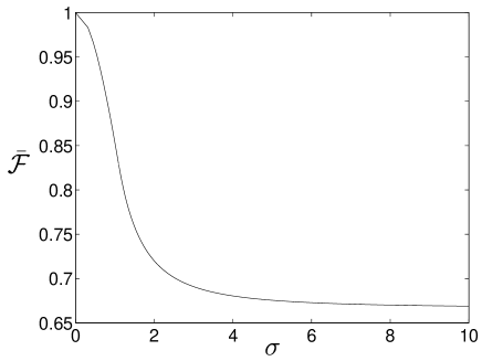
Figure 2: Average cloning fidelity $\bar{\mathcal{F}}$ (maximised over the amplifier gain) versus standard deviation of the input state probability distribution $\sigma$. The figure shows that for large $\sigma$ the average fidelity is equal to the cloning limit of $\bar{\mathcal{F}}=2/3$, and that as $\sigma$ decreases, the average fidelity increases to unity, because the prior knowledge one has of the input state becomes perfect in this limit.

Notice that at large $\sigma$, $\bar{\mathcal{F}}(\sigma)$ is at the standard cloning limit $\bar{\mathcal{F}}=2/3$. In other words, for sufficiently broad input state distributions, the situation is equivalent to having a completely arbitrary input state. As $\sigma$ decreases, the fidelity increases, because we now have better knowledge of the likely value of the input state; approaching unit fidelity as $\sigma$ tends to zero. This is an intuitive result, since if $\sigma=0$ then the input state distribution is a two-dimensional delta function in quadrature-phase space and we know with certainty the value of the input state (i.e. it is the vacuum) prior to cloning.

Notice that in Eq. (8) the minimum allowed noise added to the clones does not depend on the gain of the amplifier $G$. Our procedure of tuning the gain to find the maximum fidelity has retained this property and our clones are therefore optimal.

III.1 State estimation

We now consider the connection between cloning and optimal state estimation. Dual homodyne detection (or equivalently heterodyne detection) is known to be the optimal technique for estimating the amplitude of an unknown coherent state drawn from a Gaussian ensemble Arthurs and Kelly (1965); Yuen and Lax (1973). For our setup, dual homodyne detection of the input state would correspond to setting the amplifier gain to $G=1$, and detecting the amplitude quadrature of one of the output beams and the phase quadrature of the other. Given that we know the standard deviation of the input state distribution $\sigma$, it can be shown that the best estimate of the amplitude of the input state is given by

$$\alpha^{\prime}=\frac{1}{\sqrt{2}}\left(\frac{2\sigma^{2}}{2\sigma^{2}+1}\right)\left(\hat{X}^{+}+i\hat{X}^{-}\right),$$ (13)

where $\hat{X}^{+}$ and $\hat{X}^{-}$ are the measured values of the amplitude and phase quadratures respectively. In the limit of broad distributions ($\sigma\to\infty$) the best estimate is just given by

$$\alpha^{\prime}=\frac{1}{\sqrt{2}}\left(\hat{X}^{+}+i\hat{X}^{-}\right).$$ (14)

However, as the distribution narrows it is better to underestimate the value of $\alpha$ in accordance with Eq. (13). In the limit of $\sigma\to 0$ we become certain that $\alpha$ is zero regardless of the measurement outcome.

We have observed that the signal to noise transfer between the original state and the clones is not changed by the choice of amplifier gain, thus optimal state estimation must be possible using the clones. Some insight into the physics of the particular choice of amplifier gain which produces the optimal clones can be obtained by noticing that for optimal clones, the best estimation of the original state amplitude is determined by measuring the amplitude quadrature of one, and the phase quadrature of the other, and then setting

$$\alpha^{\prime}=\frac{1}{2}\left(\hat{X}^{+}+i\hat{X}^{-}\right).$$ (15)

This is true for all distribution sizes down to the point where the cloning amplifier gain, $G$, equals one. For even smaller distributions we return to the dual homodyne formula. At such small distribution sizes the quantum noise dominates.

III.2 Teleportation and the no-cloning limit

Teleportation is the entanglement assisted communication of quantum states through a classical channel Bennett et al. (1993). Teleportation of continuous variables Braunstein and Kimble (1998) can be achieved using entanglement of the form

$$|\psi\rangle=\sqrt{1-\lambda^{2}}\sum_{n}\lambda^{n}|n,n\rangle,$$ (16)

which describes a two-mode squeezed vacuum. The strength of the entanglement is characterised by the parameter $\lambda$ which is related to the squeezing, or noise reduction, of the quadrature variable correlations of the modes. Zero entanglement is characterised by $\lambda=0$, and maximum entanglement occurs when $\lambda=1$. Various ways to characterise the quality of the teleportation process have been proposed Braunstein et al. (2001b); Ralph and Lam (1998); Grosshans and Grangier (2001), and have been used to describe experimental demonstrations Furusawa et al. (1998); Bowen et al. (2003).

In terms of fidelity two distinct bounds have been identified for the case of an infinite input distribution of unknown coherent states. The classical limit is $\bar{\mathcal{F}}=1/2$ Furusawa et al. (1998). Fidelities higher than this value cannot be achieved in the absence of entanglement, i.e. when $\lambda=0$. The no-cloning limit on the other hand requires that the teleported version of the input state is demonstrably superior to that which could be possessed by anyone else. This is not guaranteed unless the teleported state has an average fidelity $\bar{\mathcal{F}}\geq 2/3$ Grosshans and Grangier (2001). Achieving this requires a particular quality of entanglement, $\lambda\geq 1/3$, or more than $50\%$ squeezing. We now investigate how this no-cloning limit changes as a function of the distribution of the input states.

In a previous paper Cochrane and Ralph (2003) two of us (PTC and TCR) numerically optimised the average fidelity of continuous variable teleportation of a finite Gaussian distribution of coherent input states for various levels of entanglement. An analytical expression for this optimised average fidelity is given by

$$\bar{\mathcal{F}}=\frac{1-2(\lambda^{2}-1)\sigma^{2}}{1-4(\lambda-1)\sigma^{2}},$$ (17)

where $\sigma$, as before, is the standard deviation of the input state distribution. Using this result and that derived earlier for the optimum cloning fidelity, [Eq. (11)], we can find the squeezing ($\lambda$) required for the teleportation fidelity [Eq. (17)] to equal the no-cloning limit as a function of the distribution width ($\sigma$). This is given by

$$\lambda=\left\{\begin{aligned} &\frac{8\sigma^{2}+16\sigma^{4}-2\sqrt{2}\sqrt{\sigma^{2}(2\sigma^{2}-1)(1+2\sigma^{2})^{4}}}{4\sigma^{2}+24\sigma^{4}},&\sigma^{2}\geq\frac{1}{2}+\frac{1}{\sqrt{2}}\approx 1.2\\ &\frac{6+4\sqrt{2}-\sqrt{2}\sqrt{3+2\sqrt{2}+\sigma^{2}+2\sigma^{4}}}{6+4\sqrt{2}+2\sigma^{2}},&\sigma^{2}\leq\frac{1}{2}+\frac{1}{\sqrt{2}}\approx 1.2.\end{aligned}\right.$$ (18)

The result is plotted in Fig. 3.

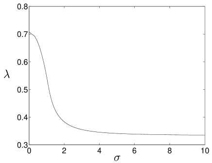
Figure 3: Entanglement required to reach the no-cloning limit as a function of the input state distribution width. The squeezing parameter $\lambda$ is plotted against the standard deviation, $\sigma$, in dimensionless units.

The maximum squeezing parameter value $\lambda=1/\sqrt{2}$ is achieved at $\sigma=0$. This is the minimum amount of squeezing required for teleportation to beat the no-cloning limit for all values of $\sigma$. Below this value it is possible for the teleportation fidelity to be lower than the no-cloning limit—and for teleported states not to be superior to that possessed by another party—for some values of $\sigma$. This is demonstrated in Fig. 4 where $\lambda=0.5$.

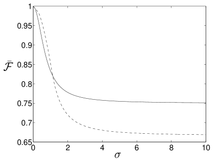
Figure 4: Teleportation fidelity $\bar{\mathcal{F}}$ (solid curve) and the no-cloning limit (dashed curve) as a function of distribution width, $\sigma$; the level of squeezing is held constant at $\lambda=0.5$. The teleportation fidelity beats the no-cloning limit for a large range of distribution widths, but dips under for $\sigma\lesssim 1$. The quantities presented are dimensionless.

The dashed curve is the no-cloning limit fidelity and the solid curve is the teleportation fidelity as a function of $\sigma$ for constant $\lambda=0.5$. Notice that for $\sigma\lesssim 1$ the teleportation fidelity drops just below the no-cloning limit. Only with $\lambda=1/\sqrt{2}$ can one be sure that one will beat the no-cloning limit.

Notice that in the limit of large $\sigma$ the teleportation fidelity is higher than the no-cloning limit and that at $\sigma=0$ the fidelity equals the no-cloning limit. The lowest constant value $\lambda$ can take and still equal the no-cloning limit at both $\sigma\rightarrow\infty$ and $\sigma=0$ is $\lambda=1/3$, corresponding to the quality of entanglement mentioned above. At lower squeezing parameter values the teleportation fidelity does not achieve the no-cloning limit except for the trivial case of $\sigma=0$.

A somewhat surprising feature is that the quality of entanglement required to reach the no-cloning limit actually increases as the width of the distribution is decreased. This occurs because of the different ways in which the teleporter and the cloner add noise at unity gain. For example for a distribution with a standard deviation $\sigma=3$, an entanglement of $\lambda=0.4$ is required, significantly higher than the $\lambda=1/3$ level of entanglement needed for an infinite distribution.

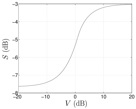
Figure 5: Entanglement required to reach the no-cloning limit as a function of the input state distribution width, as in Fig. 3. This figure plots the experimentally familiar variables of squeezing ($S$) against the variance ($V$), in units of decibels.

Fig. 5 shows the same plot as Fig. 3 but using the more experimentally familiar parameters of noise reduction (or squeezing) of the entanglement,

$$S=\frac{(1-\lambda)^{2}}{1-\lambda^{2}},$$ (19)

and the variance (or noise power) of the distribution

$$V=\sigma^{2},$$ (20)

both plotted in decibels. These graphs show that the issue of the no-cloning limit for teleportation is rather subtle when the realistic situation of finite distributions of input states is taken into account.

IV The single quadrature cloning limit

We now consider cloning of a rather different distribution of coherent states; one in which all the coherent amplitudes have the same phase, but have a broad distribution in the absolute value of their amplitudes. Effectively the signals are encoded on only one quadrature. In Sec. II we discussed the optimum cloning limit in terms of a restriction imposed by the uncertainty principle between the two conjugate parameters being copied Cerf et al. (2000). For information on a single quadrature, where only one of the conjugate observables is being copied, it could be easy to reach the naïve conclusion that there will not be such a cloning limit. However, quantum mechanics still places a restriction on the fidelity of such clones because coherent states, even when restricted to a line in phase space, are non-orthogonal. If the input states carry information on one quadrature only, a different cloning process is required. A new cloning limit, with a much higher fidelity emerges in such a scenario and is now discussed.

Consider the single quadrature Gaussian cloner shown in Fig. 6.

Figure 6: The single quadrature quantum cloner. $H$ is the OPO gain.

It consists of a phase sensitive amplifier, an optical parametric oscillator (OPO) set to amplify in the real direction Buchler (2001); Walls and Milburn (1995); Lam (1998); Lam et al. (1997, 1999), followed by a 50:50 beam splitter also made phase sensitive by the injection of squeezed vacuum noise at the dark port, $\hat{v}_{SQZ}$. The output of the OPO is given by $\sqrt{H}\hat{a}_{in}+\sqrt{H-1}\hat{a}_{in}^{\dagger}$ where $H$ is the parametric gain. After passing through the beam splitter, the variances of the output quadratures are:

$$V_{Clone1}^{\pm}\ =\ V_{Clone2}^{\pm}\ =\ \frac{V_{a}^{\pm}}{2}\ \left(\sqrt{H-1}\ \pm\sqrt{H}\right)^{2}\ +\ \frac{V_{\hat{v}}^{\pm}}{2}.$$ (21)

Suppose that the input distribution is now described by the non-symmetric Gaussian distribution

$$P(\alpha)=\frac{1}{2\pi\sigma^{2}}\exp\left(\frac{-\alpha_{x}^{2}}{2\sigma_{x}^{2}}+\frac{-\alpha_{y}^{2}}{2\sigma_{y}^{2}}\right).$$ (22)

We assume $\sigma_{y}\ll 1$, restricting the coherent states to the real axis. For simplicity we assume that the distribution “along the line” is sufficiently broad, $\sigma_{x}\gg 1$, such that fidelity will be optimized by unity gain operation. Unity gain is achieved by setting the gain to $H=\frac{9}{8}$. A minimum uncertainty state is assumed for the squeezed input noise, i.e $V_{\hat{v}}^{+}\ =\frac{1}{V_{\hat{v}}^{-}}$. This gives a fidelity of:

$$F\rightarrow\frac{2}{\sqrt{\left(\frac{5}{4}+\frac{1}{2V_{\hat{v}}^{+}}\right)\left(2\ +\frac{V_{\hat{v}}^{+}}{2}\right)}},$$ (23)

which reaches a global maximum when the beam splitter input phase is quadrature squeezed such that $V_{\hat{v}}^{-}=\sqrt{\frac{5}{8}}$, (so $V_{\hat{v}}^{+}=\sqrt{\frac{8}{5}}$). The maximum fidelity of the clone is then $\frac{4}{9}(\sqrt{10}-1)$. An equivalent result can be achieved by not injecting squeezed vacuum at the BS but instead inserting two independent OPOs in each beam splitter output arm.

The $\mathrm{SNR}^{+}$ of the individual amplitude quadrature clones is found to be:

$$\mathrm{SNR}_{out}^{+}\ =\frac{2\ \mathrm{SNR}_{in}^{+}}{(2\ +V_{\nu}^{+})}.$$ (24)

With optimised fidelity at $V_{\hat{v}}^{+}\ =\sqrt{\frac{5}{8}}$, the above expression reduces to $\mathrm{SNR}_{out}^{+}\ =\frac{5\ \mathrm{SNR}_{in}^{+}}{5\ +\sqrt{10}}\approx$ 0.6125 $\mathrm{SNR}_{in}^{+}$. This is a greater value than the single quadrature average SNR and lies outside the classical regime.

Unlike the symmetric case discussed in Sec. II, the single quadrature clones are entangled. The SNR of the summed amplitude quadratures of the clones, $X^{+}_{SUM}\ =\ X^{+}_{Clone1}\ +X^{+}_{Clone2}$, is independent of the vacuum squeezing parameter and gives $\mathrm{SNR}_{out}^{+}\ =1$. This indicates that overall no noise has been added in the cloning process. We also note that the noise outputs of the phase and amplitude quadratures are very close to the minimum uncertainty product.

It seems likely that this is the optimum fidelity attainable for coherent states on a line. The approach is analogous to the standard cloner setup, and it is hard to imagine how the phase sensitive amplification and phase sensitive beam splitter combination could be improved upon given that overall no noise is added. However, the argument is not as straightforward as for a symmetric cloner because the maximization of the fidelity is non-trivial, depending upon the phase and strength of the squeezing injected at the beam splitter. An extensive search of the parameter space revealed no better result, and we conjecture that the fidelity is optimal.

V Conclusion

We have shown how to tailor the Gaussian quantum cloner to optimally clone unknown coherent states picked from finite symmetric Gaussian distributions. Operating the cloner at a particular level below unity gain maximises the cloning fidelity for such distributions. This maximum fidelity increases monotonically as a function of the distribution width from $2/3$ in the limit of very broad distributions, to $1$ in the limit of very narrow distributions. We discussed the relationship between this optimal gain and state estimation, and have shown that the no-cloning limit for teleportation of coherent states changes in a non-trivial way as a function of the width of the input state distribution.

We have also demonstrated the existence of a qualitatively different cloning limit for coherent states on a line, and have described a machine which clones these states with a fidelity of $F=\frac{4}{9}(\sqrt{10}-1)$.