Towards mechanical entanglement in nano-electromechanical devices

Abstract

We study arrays of mechanical oscillators in the quantum domain and demonstrate how the motions of distant oscillators can be entangled without the need for control of individual oscillators and without a direct interaction between them. These oscillators are thought of as being members of an array of nano-electromechanical resonators with a voltage being applicable between neighboring resonators. Sudden non-adiabatic switching of the interaction results in a squeezing of the states of the mechanical oscillators, leading to an entanglement transport in chains of mechanical oscillators. We discuss spatial dimensions, $Q$-factors, temperatures and decoherence sources in some detail, and find a distinct robustness of the entanglement in the canonical coordinates in such a scheme. We also briefly discuss the challenging aspect of detection of the generated entanglement.

In 1959 Richard Feynman suggested in a famous talk that it appears to be a fruitful enterprise to think about manipulating and controlling mechanical devices at a very small scale. Since then, the study of micro-electromechanical (MEMS) and even nano-electromechanical systems (NEMS) has developed into a mature field of research Roukes ; Review ; Measurement ; Measurement2 ; Schwab . Mechanical oscillators with spatial dimensions of a few nanometers and very high frequencies can now be routinely manufactured. Applications of such NEMS range from mechanically-detected magnetic resonance imaging, sensing of biochemical systems, and ultrasensitive probing of thermal transport. Indeed, the NEMS devices that are presently manufactured in experimental studies are close to or already on the verge of the quantum limit Roukes ; Review ; Measurement ; Measurement2 ; Schwab . While first quantum effects are already being observed and studied, it is interesting to see to what extent it is feasible to prepare nano-scale mechanical oscillators in states where the quantum nature becomes most manifest: in states that are genuinely entangled in the canonical coordinates of position and momentum. This can be interesting for a variety of reasons. Firstly, it provides another stepping stone towards quantum state control and quantum information processing in mechanical systems. This is particularly fascinating as these systems are macroscopic consisting of many million atoms. They would therefore also permit the exploration of the limiting region between the quantum and the classical world. This might be facilitated by another application of entanglement namely its use to enhance quantum measurement schemes where entangled states represent a very sensitive probe.

The key question that will be addressed in this letter is how it is possible to entangle mechanical oscillators well separated in space, without the need for making them interact directly and with a minimum need for individual local control which is difficult to achieve at the nano-level. This will be accomplished by triggering squeezing and entanglement by a global non-adiabatic change of the interaction strength in a linear array of oscillators, but without individually addressing any of the oscillators of the array. In this way, one can achieve long-range entanglement that will persist over length scales that are much larger than the typical entanglement length for the ground state of the system Chain . The physics underlying this approach, especially the non-adiabaticity requirement, will be discussed in more detail lateron. Several schemes to probe quantum coherence of mechanical resonators in different setups and situations have been proposed so far blencowe02 ; mancini . Notably, while the earlier proposal of entangling macroscopic oscillators mancini entangles two adjacent oscillators in the context of a different physical setup, our scheme allows, without the need for individual local control, for entanglement in the canonical coordinates between non-adjacent (and possibly distant) microscopic oscillators by entanglement transport in a chain.

The setup that we will consider is an array of double-clamped coupled nano-mechanical oscillators as has been experimentally studied in the micro-mechanical realm in Ref. Buks . We assume that the beams are arranged in such a manner that between adjacent oscillators a controlled and tunable interaction can be introduced. In Ref. Buks this is experimentally achieved by applying a voltage between adjacent beams made from gold fabricated on a semiconductor membrane that are ordered alternatingly. This induces to a good approximation a nearest neighbor interaction that can be controlled in strength. The oscillators are assumed to be cooled to temperatures such that $kT/\hbar\omega\ll 1$ with $\omega$ being the fundamental frequency of the oscillators, such that the array is operated deeply in the quantum regime. Before we discuss the time and energy scales that would be required to achieve this regime, we will exemplify the mechanism, without taking sources of error and decoherence mechanisms into account, as we will discuss these in some detail later. We start with the Hamiltonian of $N$ quantum oscillators of mass $m$ and eigenfrequency $\omega$ ordered on a one-dimensional lattice, with nearest-neighbor interaction of strength $c$. Setting $\hbar=1$ and using the $q_{k}=q_{k}^{\prime}\sqrt{m\omega}$, and $p_{k}=p_{k}^{\prime}/\sqrt{m\omega}$, where $q_{k}^{\prime}$ and $p_{k}^{\prime}$ are the canonical position and momentum of the oscillators we find

$$H=\frac{\omega}{2}\sum_{k=1}^{N}\Bigl{(}p_{k}^{2}+q_{k}^{2}(1+2c)-2cq_{k}q_{k+1}\Bigr{)},$$

For the moment, we assume for simplicity periodic boundary conditions, i.e., $q_{N+1}=q_{1}$, but this requirement will be relaxed later, and set $\omega=1$, as in this ideal treatment this merely corresponds to a rescaling of the time scale. The normal coordinates are related to the previous ones by a discrete Fourier transform, $q_{k}=(1/\sqrt{N})\sum_{l=1}^{N}e^{2\pi ikl/N}Q_{l}$, $p_{k}=(1/\sqrt{N})\sum_{l=1}^{N}e^{-2\pi ikl/N}P_{l}$. In these normal coordinates, satisfying $Q_{k}=Q^{\dagger}_{N-k}$ and $P_{k}=P^{\dagger}_{N-k}$, the Hamiltonian can be written in the form

$$H=\frac{1}{2}\sum_{k=1}^{N}\left(P_{k}P_{k}^{\dagger}+(1+4c\sin^{2}(\pi k/N))^{1/2}Q_{k}Q_{k}^{\dagger}\right),$$

annihilation and creation operators, and expressing the time dependent operators $Q_{k}(t)$ and $P_{k}(t)$ in terms of these operators, one arrives at the Heisenberg equations of motion for the original canonical coordinates

$$q_{k}(t) = \sum_{r=1}^{N}(q_{r}(0)f_{r-k}(t)+p_{r}(0)g_{r-k}(t))$$

and $p_{k}(t)=\partial_{t}q_{k}(t),$ where we have defined the two functions $g_{k}(t)=\sum_{l=1}^{N}e^{2\pi ikl/N}\sin(\omega_{l}t)/(N\omega_{l})$ and $f_{k}(t)=\partial_{t}g_{k}(t)$. In this paper we are dealing with states that are Gaussian, i.e., states whose characteristic function or Wigner function is a Gaussian. As such, it is completely characterized by the first and second moments Eisert P 03 . The first moments will not be directly relevant for our purposes. The second moments can be arranged in the symmetric $2N\times 2N$-covariance matrix $\Gamma_{R,S}=2\text{Re}\langle(R-\langle R\rangle)(S-\langle S\rangle)\rangle,$ where $R$ and $S$ stand for the canonical operators $q_{1},\ldots,q_{n}$ and $p_{1},\ldots,p_{n}$. At this point, we assume that for times $t<0$, the oscillators are not interacting and are in the ground state. This implies that $\Gamma_{q_{n}q_{m}}=\Gamma_{p_{n}p_{m}}=\delta_{n,m}$, and $\Gamma_{q_{n}p_{m}}=0$, for $n,m=1,\ldots,N$.

In the setting of this paper, we will assume for $t<0$ the interaction is switched off and the system is in its ground state and time-independent. At time $t=0$ the interaction is then switched on instantaneously to ensure non-adiabaticity and consequently the system is out of equilibrium and evolving in time for $t>0$ according to the equations of motion for the second moments given by

$$\Gamma_{q_{n}q_{m}}(t)=(a_{n,m}(t)+d_{n,m}(t))/2,$$

$$\Gamma_{q_{n}p_{m}}(t)=(b_{n,m}(t)+e_{n,m}(t))/2,$$

$$\Gamma_{p_{n}p_{m}}(t)=(c_{n,m}(t)+a_{n,m}(t))/2,$$

where $a_{n,m}=\sum_{k=1}^{N}f_{k-n}f_{k-m},$ $b_{n,m}=\partial_{t}a_{m,n}/2,$ $c_{n,m}=\sum_{k=1}^{N}\partial_{t}f_{k-n}\partial_{t}f_{k-m},$, $d_{n,m}=\sum_{k=1}^{N}g_{k-n}g_{k-m},$ and $e_{n,m}=\partial_{t}d_{n,m}/2$ .

Before we discuss in detail the non-adiabaticity requirement and other idealizations as well as the physics behind this approach we demonstrate the success of the approach. We are now in the position to study the entanglement of two very distant oscillators when we ignore (trace out) all the others. The chain is translationally invariant, and hence, a single oscillator, say labeled $1$, can be singled out, and we may look at the degree of entanglement as a function of time and discrete distance. We quantify the degree of entanglement in terms of the logarithmic negativity, defined as $E_{N}(\rho)=\log\|\rho^{T_{A}}\|_{1}$ for states $\rho$, where $\rho^{T_{A}}$ is the partial transpose and $\|.\|_{1}$ denotes the trace-norm. The logarithmic negativity is an upper bound for distillable entanglement and has an interpretation of an asymptotic preparation cost and bounds the distillable entanglement Neg .

Before we consider the entanglement created in this way, let us first remind ourselves about the entanglement structure of the ground state of the harmonic lattice Hamiltonian: there, the bi-partite entanglement between two distinguished oscillators is only non-zero for nearest neighbors. Next-to-nearest neighbors are already separable for all parameters, as are more distant oscillators, even in case of an arbitrarily large correlation length of the chain when approaching criticality, as has been demonstrated in Ref. Chain .

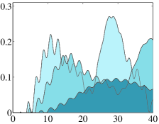
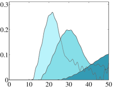
Figure 1: The degree of entanglement as a function of time between two oscillators in a chain of length $8$ with periodic boundary conditions (left) and open boundary conditions (right). On the right hand side, the first and the last oscillator in the chain are considered, on the left hand side the two diametrically opposed oscillators. The values for $c$ are in the above units $c=0.3$, $c=0.2$, and $c=0.1$ (depicted in light, medium, and dark grey).

This is very much in contrast to the situation encountered here: Astonishingly indeed, we find that even very distant oscillators become significantly entangled over time. This dependence is depicted in Fig. 1 (for periodic boundary conditions according to the above formalism, and numerically for open boundary conditions). For a time interval $[0,t_{0})$, $t_{0}>0$, the state of the oscillators with labels $1$ and $n$ is separable, then, for $t>t_{0}$ it becomes entangled. This time $t_{0}$ is approximately given by $t_{0}\approx n/(2\gamma\Omega),$ There is what can be called a finite ‘speed of propagation’ of the quantum correlations, which is in fact closely related to the speed of sound in this chain. The amount of entanglement roughly falls off as $1/n$, but becomes strictly zero after a finite distance. For $c=0.1$, for example, this happens for $n$ larger than $500$. This long-range nature of the entanglement is remarkable indeed.

The central idea behind the method above is the well-known fact that an instantaneous change in the potential of a single harmonic oscillator in its ground state will generally make its state time dependent and squeezed. In the same way a change in the coupling strength between oscillators drives the systems away from equilibrium. In the course of the subsequent time evolution the squeezing is then transformed into entanglement due to the nearest-neighbor coupling. The origin for this is the fact that the time evolution is described by a Hamiltonian quadratic in the canonical coordinates and therefore has an effect analogous to passive optical elements. It is well-known that a beamsplitter which has squeezed states as an input will lead to entangled outputs. This process happens continuously in the chain. Finally this entanglement propagates, as every other excitation, through the chain and can therefore lead to entanglement between distant sites.

In any realistic setting, this switching can not be instantaneous, and an important question is how fast the switching process must be in order to generate significant entanglement in the canonical coordinates. Fig. 2 depicts the amount of entanglement in the first maximum when the interaction strength is linearly increased over a time interval $[0,t^{\prime}]$. We find that for times $t^{\prime}<1$, any non-zero switching time is unproblematic (with very similar behavior found in longer chains). This is because the change in coupling strength is faster than any eigenfrequency in the system, preventing an adiabatic following. For very slow switching, $t^{\prime}\gg 1$, most entanglement is lost because the system can adiabatically follow the parameter change and remains approximately in the ground state.

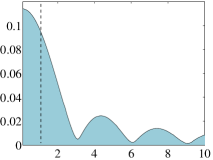
Figure 2: Maximum degree of entanglement between the end points as a function of the switching time $t^{\prime}$ in the above units for an open chain of length $8$ and $c=0.1$. The vertical dotted line represents the unit frequency of a free oscillator.

Let us now turn to the discussion of a realisation in NEMS of such an array. Presently, NEMS made from SiC have been manufactured experimentally with frequencies around $1-10$ GHz, with spatial dimensions of the order of $10$ nm Review -Yang . Doubly clamped beams have the advantage of higher fundamental frequencies with the same spatial dimensions. The $Q$-factors for NEMS of these dimensions achieve values of significantly more than $Q=10^{3}$ Higher ; QFac . Concerning the extent to which the ground state can initially be reached, cooling of the oscillators to $10$ mK seems feasible Schwab2 using a helium dilution refrigerator Roukes , Schwab (for the possibility of the equivalent of laser cooling to the ground state, see Ref. Zoller ).

Needless to say, decoherence mechanisms cannot be entirely avoided in a quantum system so close to macroscopic dimensions. After all, $Q$-factors describe nothing but the coupling strength to external degrees of freedom beyond our control. Most of the dissipation and decoherence is expected to be due to the coupling with the degrees of freedom of the substrate to which the resonator is connected. Let us now specify the decoherence model Dec : In the setting described here, we are not in the high temperature limit, but close to zero temperature. Secondly, we do not have product initial conditions: in a realistic setting, the chain and the environment are initially not in a completely uncorrelated state, but rather in the Gibbs state of the coupled joint system, and then driven away from equilibrium BroMo . We have hence modeled the decoherence process by appending local heat baths consisting of a finite number $M$ of modes to each of the oscillators with canonical coordinates $q^{k}_{j},p^{k}_{j}$ for $k=1,\ldots,M$. We choose a (discrete) Ohmic spectral density in which case the Langevin equation for the Heisenberg picture position becomes the one of classical Brownian motion in the classical limit, i.e., the coupling is specified by the interaction Hamiltonian $H_{j}=\zeta\tilde{\omega}_{j}(q_{j}\otimes\sum_{i=1}^{M}q_{j}^{i}),$ where $\tilde{\omega}_{j}=j\Lambda/M$, where $\Lambda>0$ is a cut-off frequency. This Hamiltonian induces decoherence and dissipation, and the number $\zeta>0$ has in our analysis been chosen in such a manner that the energy dissipation rate reflects exactly the rate $1/Q$ corresponding to the experimentally found $Q$-factors (see, e.g., Refs. Harrington ; Review ). With this value of $\zeta$, the initial state before switching on the interaction is then the Gibbs state of the canonical ensemble of the whole chain including the appended heat baths. The resulting map is nevertheless a Gaussian operation, such that it is sufficient to know the second moments to specify entanglement properties. This model grasps in the simplest possible manner the various noise processes Cleland in NEMS.

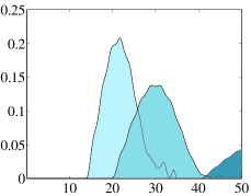
Figure 3: The degree of entanglement under decoherence and for non-zero temperature. Shown is again the situation of a chain of length $8$ for periodic (left) and open (right) boundary conditions. In this plot (up to rescaling of the time axis, and a quantification of the coupling strength $c=0.3$, $c=0.2$, and $c=0.1$ in terms of the fundamental frequency), values are chosen that correspond to the $Q$-factor $Q=10^{3}$, fundamental frequency $5$ GHz, and temperature of $10$ mK.

Fig. 3 depicts the behaviour of the degree of entanglement for system parameters that are close to those used in actual experimental settings. We see that the scheme is surprisingly robust against noise processes and non-zero temperatures. Comparably low $Q$-factors are not particularly harmful given the large speed of propagation; yet too high temperatures, turn the correlations into merely classical correlations. This effect is evidently more harmful for longer chains. Notably, for two oscillators, quite large values of the degree of entanglement can be achieved. For example, for a two-oscillator system, with system parameters as in Fig. 3, the degree of entanglement as quantified in terms of the log-negativity reaches values larger than $0.6$ for $c=0.4$. Assuming the ability to cool to $10$ mK, oscillators with fundamental frequencies of $2$ GHz would be sufficient to generate entanglement. This would be the most feasible starting point in such a scheme.

The most significant technological challenge in an experimental realization of this scheme (and actually any scheme that involves entanglement in the canonical coordinates of oscillators at the nanoscale) is the actual detection of entanglement. We would need to couple the two chosen oscillators to canonical coordinate transducers whose output is proportional to position and momentum, which is fed into an amplifier that produces a classical signal Caves . What has to be measured with very high sensitivity are the second moments of the canonical coordinates $q_{m}$, $q_{n}$, $p_{m}$, and $p_{n}$, i.e., covariance matrix elements. If not all entries can be assessed, bounds of the type $E_{N}(\rho)\geq\max\left(0,-\log((\langle(q_{n}-q_{m})^{2})\rangle+\langle(p_{n}+p_{m})^{2}\rangle)/2)\right)$ may be used to estimate the degree of entanglement. If only a position transducer is available, stroboscopic measurements may be employed where only two measurements per cycle are performed (note that $p_{m}(t=0)=q_{m}(t=\pi/4)$ and position and momentum are interchanging roles with frequency $\omega$) Caves . Alternatively, continuous single-transducer measurements may be performed which make use of only a position transducer and a sinusoidally modulated output Caves . This leaves us with the problem of measuring position and momentum with great accuracy: conventional optical transducers, as they can be employed in MEMS, are not applicable in NEMS, but near-field optical sensors or piezoelectric detectors may be used Review . Refs. Ekinci ; Measurement2 describe and make use of a balanced electronic detection scheme of displacement. The most promising to date appears to be a capacitive coupling of an electrode placed on a resonator to the gate of a single-electron transistor, as studied theoretically in Ref. blencowe00 and experimentally in Refs. Measurement ; SchwabNew . The sensitivity reached in such setups is rapidly increasing, and is presently about a factor of $4.3$ away from the quantum limit of the considered oscillator SchwabNew , while this factor was still about a 100 a year ago, and it is argued that with these techniques, the quantum limit could well be reached in the not too far future Measurement ; blencowe00 ; SchwabNew ; Schwab2 .

Finally, we would like to briefly mention that the chain of mechanical oscillators may also be used in principle as a quantum channel (compare also Ref. Bose ). If one feeds a half of a highly entangled two-mode state into a harmonic chain with nearest-neighbor interactions, then any oscillator of the chain will at some time be entangled with the kept mode. The functional behavior of the second moments as a function of time can be approximated in terms of Bessel functions Other , leading to a time $t_{1}$ of the first arrival of entanglement at the $n$-th oscillator of approximately (linear in $n$) $t_{1}\approx 2n/(\gamma\Omega e)$.

In this letter, we have presented an elementary method of entangling mechanical oscillators on the nano-scale which are located at macroscopically different locations at the ends of a chain, without the need of addressing each of the oscillators in the chain. We have introduced the suggested setup formally, and have discussed issues of decoherence and measurement. As such, the scheme is not yet a fully feasible scheme ready for experimental implementation. Yet, it is the hope that this letter can point towards significant next steps that could be taken when further exploring the quantum domain with nano-electromechanical devices.

This research was partly triggered by an inspiring talk given by M. Roukes at CalTech in January 2003. J.E. would like to thank J. Preskill and his IQI group at CalTech for kind hospitality during a research visit and S.B. would like to thank for a postdoctoral fellowship at IQI. MBP is supported by a Royal Society Leverhulme Trust Senior Research Fellowship. We would like to thank K. Schwab, M. Roukes, I. Wilson-Rae, P. Rabl, and C. Henkel for interesting communication. This work has been supported by the EU (QUPRODIS), the DFG, the US Army (DAAD 19-02-0161), and the EPSRC QIP-IRC.

References

- (1) M. Roukes, Phys. World 14, 25 (2001); H.G. Craighhead, Science 290, 1532 (2000).
- (2) M. Roukes, Technical Digest of the 2000 Solid-State Sensor and Actuator Workshop (2000), cond-mat/0008187.
- (3) R.G. Knobel and A.N. Cleland, Nature 424, 291 (2003).
- (4) X.M.H. Huang, C.A. Zorman, M. Mahregany, and M.L. Roukes, Nature 421, 496 (2003).
- (5) K.C. Schwab, E.A. Henriksen, J.M. Worlock, and M.L. Roukes, Nature 404, 974 (2000).
- (6) K. Audenaert, J. Eisert, M.B. Plenio, and R.F. Werner, Phys. Rev. A 66, 042327 (2002).
- (7) A.D. Armour, M.P. Blencowe, and K.C. Schwab, Phys. Rev. Lett. 88, 148301 (2002); W. Marshall, C. Simon, R. Penrose, and D. Bouwmeester, ibid. 91, 130401 (2003).
- (8) S. Mancini, V. Giovannetti, D. Vitali, and P. Tombesi, Phys. Rev. Lett. 88, 120401 (2002).
- (9) E. Buks and M.L. Roukes, JMEMS 11, 802 (2002).
- (10) J.J. Halliwell, Phys. Rev. D 68, 025018 (2003).
- (11) J. Eisert and M.B. Plenio, Int. J. Quant. Inf. 1, 479 (2003).
- (12) K. Zyczkowski, P. Horodecki, A. Sanpera, and M. Lewenstein, Phys. Rev. A 58, 883 (1998); J. Eisert and M.B. Plenio, J. Mod. Opt. 46, 145 (1999); J. Eisert (PhD thesis, Potsdam, February 2001); G. Vidal and R.F. Werner, Phys. Rev. A 65, 032314 (2002); K. Audenaert, M.B. Plenio, and J. Eisert, Phys. Rev. Lett. 90, 027901 (2003).
- (13) Y.T. Yang, K.L. Ekinci, X.M.H. Huang, L.M. Schiavone, and M.L. Roukes, Appl. Phys. Lett. 78, 162 (2001).
- (14) The larger the spatial dimensions, the larger are the -factors that have been achieved. The logarithms of the best known -factors are approximately linear in the logarithm of the volume of the mechanical resonators Review .
- (15) The -factor specifies the dissipation of energy to other modes in an uncontrolled manner. It is the number of radians of oscillations necessary for the energy to decrease by a factor of .
- (16) K. Schwab, private communication.
- (17) I. Wilson-Rae, P. Zoller, and A. Imamoglu, Phys. Rev. Lett. 92, 075507 (2004).
- (18) W.H. Zurek, Rev. Mod. Phys. 75, 715 (2003); D. Giulini et al., Decoherence and the Appearance of a Classical World in Quantum Theory (Springer, Heidelberg, 1996); A.O. Caldeira and A.J. Leggett, Physica A 121, 587 (1983).
- (19) Therefore, we have not modeled decoherence by merely appending local terms reflecting decoherence in position to the generators of the dynamical map with suitable (corresponding to the approximation of the exact generator in Ref. Hu in the limit of very weak damping to the extent of neglible friction, very high temperatures, Ohmic spectral density, and factorizing initial conditions), which is not necessarily appropriate, due to the non-factorizing initial conditions.
- (20) B.L. Hu, J.P. Paz, and Y. Zhang, Phys. Rev. D 45, 2843 (1992).
- (21) A.N. Cleland and M.L. Roukes, J. Appl. Phys. 92, 2758 (2002).
- (22) D.A. Harrington, P. Mohanty, and M.L. Roukes, Physica B 284, 2145 (2000).
- (23) M.B. Plenio, J. Hartley and J. Eisert, New J. Phys. 6, 36 (2004).
- (24) M.P. Blencowe and M.N. Wybourne, Appl. Phys. Lett. 77, 3485 (2000).
- (25) C.M. Caves et al., Rev. Mod. Phys. 52, 341 (1980).
- (26) K.L. Ekinci, Y.T. Yang, X.M.H. Huang, and M.L. Roukes, Appl. Phys. Lett. 81, 3879 (2002).
- (27) M.D. LaHaye, O. Buu, B. Camarota, and K.C. Schwab, Science 304, 74 (2004).
- (28) S. Bose, Phys. Rev. Lett. 91, 207901 (2003).