Quantum fluctuations and correlations of spatial scalar or multimode vector solitons in Kerr media

Abstract

We apply the Green’s function method to determine the global degree of squeezing and the transverse spatial distribution of quantum fluctuations of solitons in Kerr media. We show that both scalar bright solitons and multimode vector solitons experience strong squeezing on the optimal quadrature. For vector solitons, this squeezing is shown to result from an almost perfect anti-correlation between the fluctuations on the two incoherently-coupled circular polarisations.

1 Introduction

The analysis of spatial aspects of quantum fluctuations is now a well established field of quantum optics (see for example [1] for a review). More specifically, some recent studies [2, 3, 4] have considered quantum effects in spatial solitons. Ref. [2] shows that vacuum-induced jitter remains negligible versus the width of a soliton. In Ref. [3], production of subpoissonian light is demonstrated by placing either a stop on the centre of the beam in the near field or a low pass filter in the far-field. These two theoretical papers use linearisation of quantum fluctuations. Ref. [4] gives a general method to numerically determine the transverse distribution of linearised quantum fluctuations by using Green functions. Results show an important global squeezing for $\chi^{2}$ as well as for $\chi^{3}$ solitons. In Kerr media however, this squeezing does not occur on the amplitude quadrature, implying homodyne detection. Ref.[4] demonstrates also local squeezing and anti-correlations between different parts of the beam. The Green’s function method has also been applied to the assessment of spatial aspects of quantum fluctuations of spontaneous down-conversion [5]. In this paper, we apply the Green’s function method to spatial scalar solitons and to multimode vector solitons in Kerr media [6, 7]. The results for the scalar solitons appear somewhat different of that given in ref. [4], because of a flaw in the numerics used in this reference. We show in particular that, in the corrected results, the squeezing monotonically increases with the propagation length, like for a plane wave. We show also that results of ref. [3] are retrieved with the Green’s function method.

We study also the quantum properties of multimode vector solitons that result from incoherent coupling of two counter-rotating circularly polarised fields mutually trapped through cross-phase modulation, the self-focusing nature of a component being exactly compensated by the diffracting nature of the other. We find the quantum limits for the stability of these multimode vector solitons and show that the global squeezing (measured on the total intensity of the soliton) appears to be similar to that of scalar solitons. In addition, we demonstrate that there exists a strong anti-correlation between the circular components.

The paper is organised as follows. In Sec. 2, we recall the principle of the Green’s function method. Sec. 3 gives the results for scalar Kerr solitons and Sec. 4 is devoted to vector solitons.

2 Green’s function method

Let us briefly recall the main features of the Green’s function method [4] that allows us to determine the spatial distribution of quantum fluctuations in the regime of free propagation in a non-linear medium. We will present it in the simplest case of a scalar field and in the configuration of a single transverse coordinate x. The classical propagation equation for the complex electric field envelope $U(x,z)$ is in this case :

$$\frac{\partial U}{\partial z}=\frac{i}{2k}\frac{\partial^{2}U}{\partial x^{2}}+i\gamma|U|^{2}U$$ (1)

where $\gamma$ is the usual Kerr coefficient, z the main propagation direction, $k$ the longitudinal wavevector, and x the transverse position in the transverse plane. This equation has a solution that we will call $\bar{U}(x,z)$.

Let us write the quantum positive frequency operator describing the same field at the quantum level, $\hat{U}(x,z)$, as :

$$\hat{U}(x,z)=\bar{U}(x,z)+\delta\hat{U}(x,z)$$ (2)

If the fluctuations remain small compared to the mean fields, which is true as long as the field contains a macroscopic number of photons, then the quantum mean field coincides with the field given by classical nonlinear optics, $\bar{U}(x,z)$, and the fluctuations $\delta\hat{U}$ obey a simple propagation equation, obtained by linearizing the classical equation of propagation 2 around the mean field. This equation writes :

$$\frac{\partial}{\partial z}\delta\hat{U}=\frac{i}{2k}\frac{\partial^{2}}{\partial x^{2}}\delta\hat{U}+i\gamma\left(2|\bar{U}|^{2}\delta\hat{U}+\bar{U}^{2}\delta\hat{U}^{+}\right)$$ (3)

As this equation is linear, one can use Green’s function techniques to solve it. Its solution at a given $z_{out}$ is a linear combination of the input fluctuations operators in plane $z_{in}$:

$$\delta\hat{U}(x,z_{out})=\int dx^{\prime}G(x,x^{\prime})\delta\hat{U}(x^{\prime},z_{in})+\int dx^{\prime}H(x,x^{\prime})\delta\hat{U}^{+}(x^{\prime},z_{in})$$ (4)

where $G(x,x^{\prime})$ and $H(x,x^{\prime})$ are the Green’s functions associated with the linear propagation equation 3. If the input field fluctuations are those of a vacuum field, or of a coherent field, they are such that :

$$<\delta\hat{U}(x,z_{in})\delta\hat{U}^{+}(x^{\prime},z_{in})>=C\delta(x-x^{\prime})$$ (5)

where $C$ is a constant. Equations 4 and 5 allow us to calculate quantum noise variance or correlation at the output of our system on any quadrature component when one knows the two Green’s function $G(x,x^{\prime})$ and $H(x,x^{\prime})$ of the problem. These two functions can readily be numerically calculated as solutions of the propagation equation 3 when the initial condition is a delta function localised at a given transverse point. This method can be obviously extended to any kind of non-linear propagation equation.

We will focus our attention here on two kinds of simple spatially resolved measurements : the first one is the direct photodetection on a pixellised detector, which gives access to the local intensity fluctuations ; the second one is the spatially resolved balanced homodyne detection, using a local oscillator having a plane wavefront, coincident with the detector plane and with a global adjustable phase $\theta$, which allows us to measure the local fluctuations $\delta\hat{I}(\theta,x)$ of a given quadrature component. Reference [4] gives the mathematical expressions, in terms of the Green’s functions $G(x,x^{\prime})$ and $H(x,x^{\prime})$, of these quantities, from which one easily derives the best local squeezing $min_{\theta}<(\delta\hat{I}(\theta,x))^{2}>$ and the covariance between pixels :

$$C(x,x^{\prime},\theta)={<\delta\hat{I}(\theta,x)\delta\hat{I}(\theta,x^{\prime})>}$$ (6)

3 Results : scalar solitons

Equation (1) describes the propagation of the electric field envelope of a monochromatic field of frequency $\omega$ in a planar waveguide made of a Kerr medium, i.e. having an intensity dependent index of refraction:

$$n=n_{0}+n_{2}|U|^{2}$$ (7)

with $k=n_{0}\omega/c$ and $\gamma=n_{2}\omega/c$.

It can be written in a universal form if one uses a scaling parameter $\eta$ and the scaled variables $\zeta=\eta z$, $r=x\sqrt{2\eta k}$, and its solution is the well known $\zeta$ invariant hyperbolic secant proportional to $1/coshr$ : the 1D scalar soliton, which is able to propagate without deformation in the nonlinear medium.

3.1 Squeezing on the total beam

As it is well known [12], the Kerr effect produces in the plane-wave case a significant amount of squeezing, which increases monotonously with the propagation distance. The squeezing is optimized for a given quadrature component (best squeezing) which is neither the amplitude nor the phase quadrature. However, the amplitude quadrature of the field remains at the shot noise level. Fig 1 gives the results of the Green’s function method for the scalar soliton, and shows that the results are quite similar to the plane wave case, in the case of a photodetector having an area much larger than the soliton spot. Neglecting diffraction, or using single mode propagation in an optical fiber [8, 9, 10, 11] seems almost equivalent to compensating diffraction by self-focusing, for a given nonlinear phase $\zeta$. Hence a spatial soliton appears as a practical mean to obtain strong squeezing, with the restriction that it must be detected by homodyne techniques.

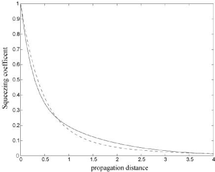
Figure 1: Best total squeezing, in shot-noise units, observed on the Kerr scalar soliton (solid line), versus the normalized propagation distance. The dotted line corresponds to the plane wave case. In both cases, the normalized propagation distance corresponds to the nonlinear phase $\zeta$.

3.2 Local quantum fluctuations.

In order to measure the local quantum fluctuations, we use a homodyne detector, made of photodetectors of very small area and quantum efficiency 1, and using a local oscillator at frequency $\omega$, placed at the output of the nonlinear medium, which is able to monitor the quantum noise on any quadrature component at point $(x,z_{out})$ and we vary the local oscillator phase to reach the minimum noise level : we obtain by this way a quantity that we call ”best squeezing”. Figures (2a) and (2b) give, for two normalized propagation distances ($\zeta=0.3$ and $\zeta=3$), such a quantity as a function of x, together with the phase angle of the local oscillator enabling us to reach the best squeezed quadrature. One observes that the central pixel is the most squeezed. However, the noise level appears to be above the shot noise for the longer propagation length.

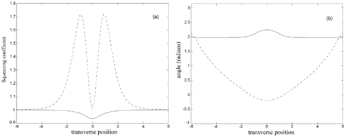
Figure 2: (a) Best total squeezing in shot-noise units, and (b) corresponding angles, observed on a single pixel, versus its transverse position. Solid line : for a propagation distance equal to 0.3 Ld. Dashed line : for a propagation distance equal to 3 Ld.

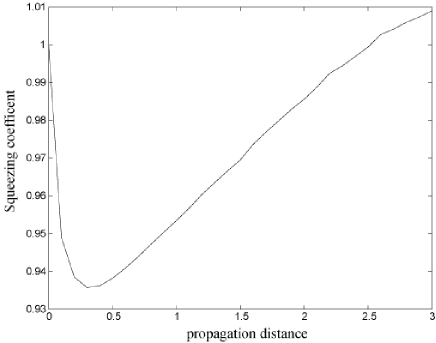
Figure 3: Best total squeezing, in shot-noise units, observed on the central single pixel, versus the propagation distance.

Indeed, figure 3, which displays the variation of the best squeezing on the central pixel as a function of propagation length, shows that the fluctuations on this pixel decrease until an optimal propagation length ($\zeta=0.3$), then increase and overpass the shot noise for a sufficiently long propagation length. Hence, long propagation lengths produce at the same time a local excess noise and a squeezed total beam (see fig.1). These results are not contradictory because, as we will soon see, there is a gradual build-up of anti-correlations between the different transverse parts of the soliton because of diffraction.

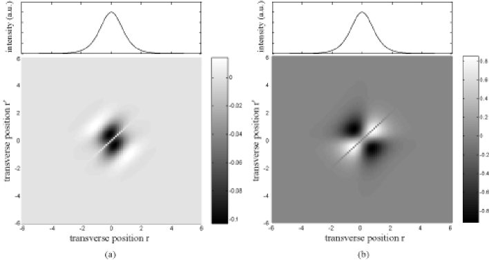
Figure 4: bottom: Covariance $C(x,x^{\prime},\theta)$ between pixels on the best squeezed quadrature for (a) a propagation distance of 0.3 Ld and (b) a propagation distance of 3 Ld. The values on the main diagonal (variance) have been removed. Top : Corresponding transverse intensity profile of the scalar soliton.

Figure 4 shows that the covariance between pixels on the best squeezed quadrature (calculated with eq.6 and where best squeezing is defined for the total beam) increases and spreads out when passing from $\zeta=0.3$ to $\zeta=3$. Indeed, only pixels close to each other are anti-correlated for $\zeta=0.3$ while the correlation between adjacent pixels becomes positive for $\zeta=3$. For this latter distance, squeezing is due to the anti-correlation between the left and the right side of the soliton.

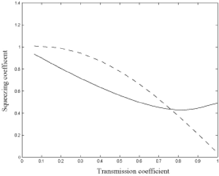
Figure 5: Best squeezing for a photodetector of variable size, versus the transmission coefficient defined as the ratio between the detected and the total intensity. Solid line : for a propagation distance of 0.3 Ld. Dashed line : for a propagation distance of 3 Ld.

Figure 5 shows the best squeezing for a photodetector of variable size, centered on the beam. This photodetector can be seen as an iris that allows the detection of only the central part of the beam, with a minimum size corresponding to the central pixel and a maximum size corresponding to the detection of the entire beam. As expected, the noise on a very small area is close to the shot noise. The squeezing on a small central area is bigger at small distance, while the squeezing for the entire beam is better at great distance. For $\zeta=0.3$ the squeezing is maximum for a finite size of the photodetector (transmission coefficient of 0.8, corresponding to a normalized radius of 1), while detecting the entire beam ensures the maximum squeezing for $\zeta=3$.

In many circumstances, a spatial soliton behaves as a single mode object. The present analysis allows us to check such a single mode character at the quantum level : let us assume that the system is in a single mode quantum state. This means that it is described by the state vector $|\Psi>\otimes|0>\otimes...\otimes|0>...$, $|\Psi>$ being a quantum state of the mode having the exact spatial variation of the soliton field, and all the other modes being in the vacuum state. It has been shown in [13] that if a light beam is described by such a vector, then the noise recorded on a large photodetector with an iris of variable size in front of it has a linear variation with the iris transmission. We see in figure 5 that it is not strictly speaking the case : as far as its quantum noise distribution is concerned, a spatial soliton is not a single mode object. Let us also notice that the departure from the linear variation is on the order of $10\%$, so that the single mode approach of the soliton remains a good approximation.

3.3 Intensity squeezing by spatial filtering

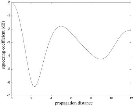
Figure 6: : intensity squeezing, in dB, for a photodetector placed at the center of the Fourier plane, with a total width of 0.25 in units of spatial frequencies corresponding to the normalized units of the direct space.

In all results presented in the preceding paragraph, squeezing can be measured only by homodyne detection, because no squeezing is present for the amplitude quadrature, which is the easiest to measure, as it requires only direct detection, and no interferometer. Actually, Mecozzi and Kumar [3] have shown that a simple stop on the central part of the soliton beam ensures intensity squeezing on the remaining of the light. They have proposed the following intuitive explanation : if the intensity fluctuation is positive for the entire beam, the soliton becomes narrower (its width is inversely proportional to its power) and the stop will produce larger losses. In the Fourier plane, a square diaphragm (low-pass filter) will produce an even better squeezing. Figure 6 shows the intensity squeezing we have obtained with the Green’s function method by considering an aperture placed in the Fourier plane. These results are in full agreement with the fig. 1 of Ref. 3, that uses another linearisation method. The residual differences come probably from a small difference in the aperture width. To conclude this paragraph, we find, as Mecozzi and Kumar, that subpoissonian light can be very easily produced from a spatial soliton by placing a simple aperture in the Fourier plane.

4 Quantum limits of stability and squeezing on vector solitons

4.1 Multimode vector solitons and symmetry-breaking instability

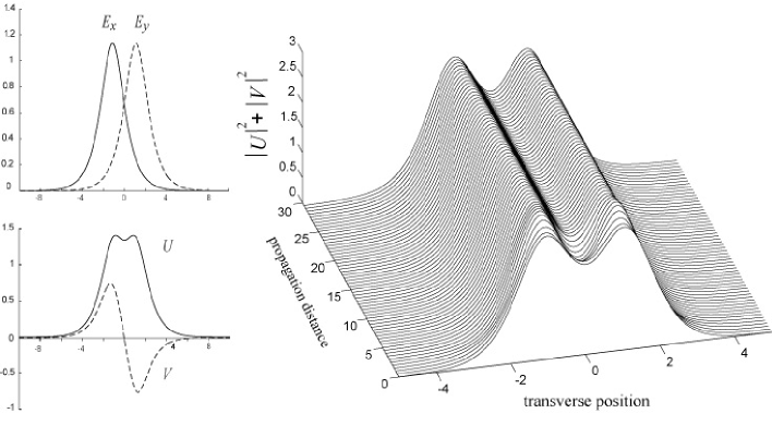
Figure 7: Vector soliton projected either on orthogonal linear polarisations ($E_{x}$ and $E_{y}$) or on counter-rotating circular polarisations (U and V). The right plot shows invariant propagation of the soliton bound-state.

In the last few years, a great number of multi-component solitons have been demonstrated [14]. Among these, the simplest example is the bimodal vector soliton which is depicted in fig. 7a and consists of two opposite circular components that trap each other in a non birefringent Kerr medium. Their complex envelopes U and V obey the following coupled nonlinear Schrödinger equations :

$$\cases{\frac{\partial U}{\partial Z}=i\frac{1}{2k}\frac{\partial^{2}U}{\partial x^{2}}+i\gamma(|U|^{2}U+7|V|^{2}U)\\ \frac{\partial V}{\partial Z}=i\frac{1}{2k}\frac{\partial^{2}V}{\partial x^{2}}+i\gamma(|V|^{2}V+7|U|^{2}V)\\ }$$ (8)

Where $\gamma$ is the usual Kerr coefficient, and 7 represents the strength of the cross-phase modulation in an isotropic liquid, like $CS_{2}$ [15]. As can be seen on fig.7b, this soliton bound-state propagates in equilibrium due to incoherent coupling between both circular components. If alone in the Kerr medium, the symmetrical field U tends to self-focus. However, the antisymmetrical field V on the counter-rotating polarization tends to diffract and it can be shown that a proper choice of the intensities (in dimensionless units on Figs 7) ensures an exact balance between diffraction and self-focusing. However, this equilibrium is unstable if the cross-phase modulation coefficient is greater than the self-phase modulation coefficient. Figure 8a displays the solution of the classical equations of propagation when a very small spatial initial asymmetry is introduced in one of the two fields. It shows that the multimode soliton is unstable and eventually collapses, the intensity evenly distributed between the two cores of the induced waveguide going abruptly from one core to the other. The instability occurs after a propagation distance that decreases as the initial asymmetry increases, as it can be clearly seen in fig. 8b. A more complete description of this phenomenon is given in Ref. [6], while the first experiment demonstrating symmetry-breaking instability is reported in Ref. [7]. In this experiment, performed with pulses issued from Nd-Yag at a 10 Hz repetition rate, symmetry-breaking induced by the noise at the input occurred for about $60\%$ of the laser shots, with a left-right repartition equally and randomly distributed.

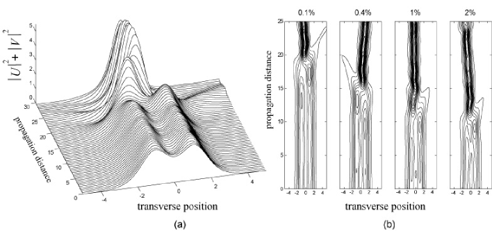
Figure 8: (a) Symmetry-breaking instability of the bimodal soliton represented in 3-D., and (b) the same in level curves for different initial asymmetry levels at the input

4.2 Stability of vector solitons : quantum limits

Propagation of a multimode vector soliton in a medium with strong cross phase-modulation is unstable, as shown theoretically by Kockaert et al. [6], using a linear stability analysis. Because of quantum noise, symmetry-breaking will occur even for an ideal symmetrical input beam. The simplest way to quantitatively assess the phenomenon is propagating a vector soliton, using Eq.(8) and the usual split-step Fourier method, after the addition on the input fields of a Gaussian white noise with a variance of half a photon per pixel on each polarization. The validity of such type of stochastic simulation is well known in the framework of the Wigner formalism [16]. Results show symmetry-breaking with a random direction after 60 to 70 diffraction lengths.

A linear stability analysis [6] shows that exponential amplification occurs only for the part of the input noise obtained by projection on the eigenvectors associated to eigenvalues with a negative imaginary part. Such an eigenvector corresponds physically to a transverse distribution of field for each circular polarization. The part of an unstable eigenvector that is circularly polarized as the U symmetrical field is antisymmetrical, while the part of the eigenvector that is circularly polarized as the V antisymmetrical field is symmetrical. Moreover, exponential amplification corresponding to the eigenvalue having the most negative imaginary part is predominant after a short propagation distance. Hence, instability can be described as the amplification of a single unstable eigenvector. In the results of figure 9, the field corresponding to this eigenvector with an energy of half a photon per polarization has been added at the input to the ideal vector soliton. Figure 9 shows in solid line the evolution of the norm of the difference between the input field and the propagated field, compared to a pure exponential amplification with the corresponding imaginary eigenvalue (dashed line). The difference evolves almost exponentially, with however a periodic modulation due to the real part of the eigenvalue. This phase modulation leads to a dependence between the direction of symmetry-breaking and the initial amplitude of the perturbation. Symmetry-breaking appears clearly on figure 9 when the initial small perturbation has grown until a macroscopic level, for a propagation distance of about 70 diffraction lengths.

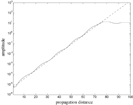
Figure 9: Solid line : norm of the difference between the unperturbed and the perturbed field, versus the propagation distance. The input perturbation corresponds to the unstable eigenvector. Dashed line : exponential amplification with the corresponding eigenvalue.

To conclude this paragraph, the usual classical simulation of quantum noise allows us to predict a maximum propagation length for the multimode vector soliton. This length is less than two meters, for the diffraction length characterizing the experiment of ref.[7], but also 70 times the typical length leading to symmetry-breaking in this experiment. Actually, experimental evidence of quantum limits for symmetry-breaking appears as a rather difficult challenge, because unavoidable spatial classical noise dominates in realistic input fields.

4.3 Total beam squeezing and correlation between polarisations

In this paragraph, we give the results of the Green’s function method in the case of vector solitons. Because these solitons are not analytically integrable, the impulse response due to a Dirac-like field modification of the perfect vector soliton is more complicated to determine, and calculated as follows. The perturbation consists in a unity single-pixel step, multiplied by a small coefficient before to be added to the field in order to ensure a near-perfect linearity of propagation equations for the perturbation. Both the unmodified and the modified field are first numerically propagated using eq.8, then subtracted each other. Finally, the subtraction result is divided by the initial multiplication coefficient, in order to retrieve the output corresponding to the input unity single-pixel step. An important point is that the phase reference corresponding to the amplitude quadrature is given for each pixel by the unmodified field. Indeed, in practice the vector soliton could experience a very slight breathing, that results in a weak phase curvature. Therefore, taking the mean soliton phase as reference leads to strong numerical inaccuracies for strong squeezing.

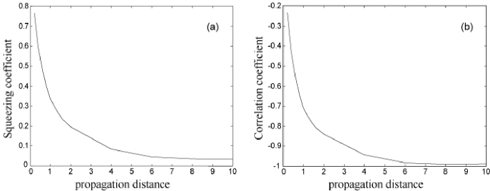
Figure 10: : best total squeezing in shot-noise units (a) and correlation coefficient between circular polarisations (b) versus the normalized propagation distance.

Fig 10 shows the global squeezing coefficient of the vector soliton on the best quadrature. This figure is very similar to that obtained for a scalar soliton (figure 1) : strong squeezing occurs, although somewhat smaller than in the scalar case for the same propagation distance. However, this squeezing is due to a strong anti-correlation between circular components, as shown in figure 10 b. It can be verified on figure 11, which displays the best squeezing of each circular polarisation component as a function of propagation, that the best squeezing on a single circular polarization is much weaker. We can conclude that a vector soliton as a whole exhibits quantum properties that are similar to a scalar soliton, while the field on each polarisation does not constitute itself a soliton.

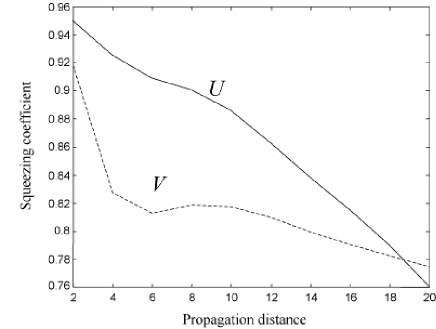
Figure 11: : best squeezing in shot-noise units on each circular polarisation versus the normalized propagation distance.

4.4 Local quantum fluctuations

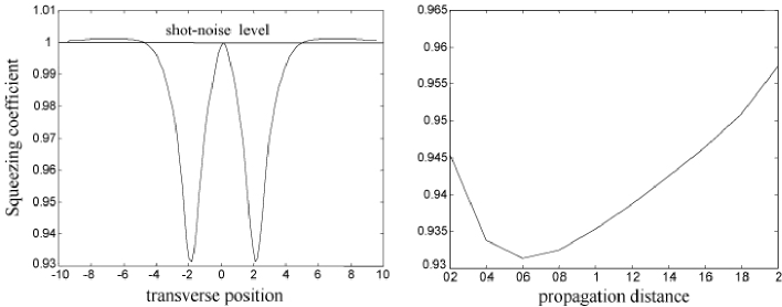
Figure 12: best squeezing on one pixel. a : versus the transverse position for $\zeta$ = 0.6. b : versus the propagation distance for the transverse position corresponding to the strongest squeezing

Figure 12 shows the squeezing coefficient on one pixel versus its transverse position, for the propagation length where this local squeezing is the most intense. The degree of squeezing is similar to the scalar case (see figure 2), with however two peaks of squeezing located on the intensity peaks of the multimode vector soliton. As in the scalar case, local squeezing is maximum for a relatively small propagation length (fig.12 b). Figure 13 shows the best squeezing for a photodetector of variable size, centered on one of the intensity peaks. In contrast to figure (5) the variation is far from being linear with the transmission, meaning that the system is not single mode, as expected. One observes that for long propagation distances, the global squeezing reaches a maximum for a photodetector size corresponding roughly to the peak width. This global squeezing implies the existence of spatial anti-correlations. Indeed, the local squeezing on one pixel disappears for such long distances (see figures 12 and 13).

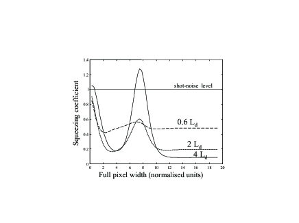
Figure 13: Best squeezing for a photodetector centered on one intensity peak and of variable size, for 3 different propagation distances, versus the transmission coefficient defined as the ratio between the detected and the total intensity.

The correlations between fluctuations at different pixels, and possibly on different polarizations, provide a great deal of information about the distribution of fluctuations in the soliton. Figure 14 shows these spatial correlations, in terms of the covariance functions $C(x,x^{\prime},\theta)$ of the two polarizations, and the covariance function between the two modes, on the best squeezed quadrature and for 2 propagation lengths. One sees that for $\zeta=0.6Ld$, anti-correlations appear between pixels when one measures different circular polarizations on the pixels. It means that the effect of cross-phase modulation is already noticeable, while effects of diffraction and self-phase modulation are still weak. For $\zeta=2Ld$, anticorrelations appear also between pixels on the same polarization, as for the scalar soliton.

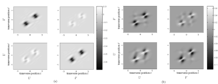
Figure 14: Covariance $C(x,x^{\prime},\theta)$, in shot-noise units, between pixels on the best squeezed quadrature for two propagation distances (a) 0.6 Ld and (b) 2 Ld. The values on the main diagonal (variance) have been removed.

4.5 Fluctuations on linear polarisations

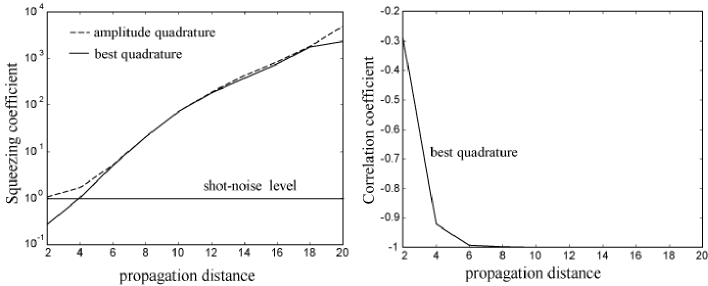
Figure 15: Squeezing coefficient (a) and correlation coefficient (b) of linear polarisations versus the propagation distance.

Figure 15 shows that squeezing on linear polarisations disappears after a relatively short propagation distance, even on the best quadrature. Moreover, fluctuations grow exponentially. On the other hand, fluctuations on both linear polarisations are perfectly anti-correlated after some distance, as it was expected because of the strong squeezing of the global beam. We have verified that the results on this global beam (section 4.3) can be retrieved also from a description of the field by projection on linear polarisations.

5 Conclusion

Let us summarise here the main results about the spatial distribution of quantum fluctuations in 1D Kerr solitons that we have obtained in this paper : as far as measurements on the whole soliton are considered, we have shown that scalar Kerr solitons, as well as vector Kerr solitons, exhibit squeezing properties similar to that of a plane wave propagating in the same medium and for the same type of propagation distance. Because of diffraction, as the soliton propagates, strong anti-correlations develop between symmetrical points inside the scalar soliton spot, and between polarisation components for the vector soliton.

6 Acknowledgments

This work has been supported by the European Union in the frame of the QUANTIM network (contract IST 2000-26019).

7 References

References

- [1] M.I. Kolobov, Rev. Mod. Phys. 71,1539 (1999).
- [2] E.M. Nagasako, R.W. Boyd, G.S. Agrawal, Optics Express 3 171-179 (1998)
- [3] A. Mecozzi, P. Kumar, Quantum and Semiclassical Optics 10 L21-L26 (1998)
- [4] N. Treps and C. Fabre, Phys. Rev. A 62 033816 (2000)
- [5] E. Lantz, N. Treps, C. Fabre, E. Brambilla, ”Spatial distribution of quantum fluctuations in spontaneous down-conversion in realistic situations : comparison between the stochastic approach and the Green’s function method.” , submitted
- [6] P. Kockaert, M. Haeltermann, J. Opt. Soc. Am. B 16 732-740 (1999)
- [7] C. Cambournac, T. Sylvestre, H. Maillotte, B. Vanderlinden, P. Kockaert, Ph. Emplit, and M. Haelterman, Physical Review Letters 89 083901 (2002)
- [8] R. Shelby, M. Levenson, S. Perlmutter, R. De Voe, D. Walls, Phys. Rev. Lett. 57 681 (1986)
- [9] K. Bergman, H. Haus, Optics Lett. 16 663 (1991)
- [10] S. Friberg, S. Machida, Y. Yamamoto, Phys. Rev. Lett. 69 3775 (1992)
- [11] S. Spalter, N. Korolkova, F. Konig, A. Sizmann, and G. Leuchs, Phys. Rev. Lett. 81 786 (1998)
- [12] M. Kitagawa, Y. Yamamoto, Phys. Rev. A 34 3974 (1986)
- [13] M. Martinelli, N. Treps, S. Ducci, S. Gigan, A. Maitre, C. Fabre, Phys. Rev. A 67 023808 (20003)
- [14] Y.S. Kivshar and G.P. Agrawal, Optical solitons : From fibers to Photonic Crystals, (Academic Press, San Diego, 2003).
- [15] R.W. Boyd, Nonlinear optics, (Academic Press, San Diego, 1992).
- [16] E. Brambilla, A.Gatti, M. Bache and L.A.Lugiato, ”Simultaneous near-field and far field spatial quantum correlations in spontaneous parametric down-conversion”, submitted.