Diverging Entanglement Length in Gapped Quantum Spin Systems

Abstract

We prove the existence of gapped quantum Hamiltonians whose ground states exhibit an infinite entanglement length, as opposed to their finite correlation length. Using the concept of entanglement swapping, the localizable entanglement is calculated exactly for valence bond and finitely correlated states, and the existence of the so–called string-order parameter is discussed. We also report on evidence that the ground state of an antiferromagnetic chain can be used as a perfect quantum channel if local measurements on the individual spins can be implemented.

The fields of Condensed Matter and Quantum Information Theory share a common interest in the study of quantum states of many–body systems. Much of the current effort in Quantum Information Theory is devoted to the description and quantification of the entanglement contained in quantum states in general: this intriguing property of Quantum Mechanics is the basic resource of most of the applications in this field, including quantum communication and computation. Condensed matter theory, on the other hand, is deeply interested in the strongly correlated states appearing in certain materials at very low temperatures, since they describe a variety of fascinating phenomena, like the ones occurring in quantum phase transitions and superconductivity.

Despite the fact that the number of parameters to describe a quantum state scales exponentially in the number of particles, it is sometimes possible to capture the most relevant physical properties by describing these systems in terms of very few parameters. In the case of spin chains, for example, two–particle correlations play a fundamental role. They allow us to understand several complex physical phenomena, like phase transitions and the appearance of a length scale in the system. Much insight has also been obtained by studying exactly solvable models such as the AKLT-model AKLT , which illustrates the appearance of the Haldane gap Haldane in spin–1 antiferromagnets and the associated finite correlation length.

From the perspective of entanglement theory, the presence of two-particle correlations between two distant particles in a many-particle pure state guarantees the possibility of establishing EPR-type entanglement between them by doing local measurements on the other particles VPC03 . On the other hand, highly entangled multiparticle pure states typically have reduced two-particle density operators close to the maximally mixed state and therefore only exhibit very small correlations. Correlation functions can therefore only reveal partial information about the long-range quantum correlations that ought to be present in a state. The so–called Localizable Entanglement (LE) VPC03 between two particles is defined as the maximal possible bipartite entanglement that can be localized between them, on average, by optimizing over all possible local measurements on the other particles. The LE has a very clear operational meaning as it quantifies the amount of entanglement that can be localized at e.g. the end points of a spin chain and that could be used, e.g., as a perfect quantum channel. Just as correlation functions induce a correlation length $\xi_{C}$ in a lattice, the LE induces a new length scale which we call the entanglement length $\xi_{E}$. It has been proved in VPC03 that $\xi_{E}\geq\xi_{C}$; therefore a diverging correlation length at e.g. a quantum phase transition implies a diverging entanglement length. In the case of ground states of typical spin–$1/2$ systems such as the Ising chain and the Heisenberg antiferromagnet in a magnetic field, we observed that the bound is tight $\xi_{E}=\xi_{C}$ Popp and hence the opposite also holds true in this case. This triggered the quest for a phase transition that is detected by a diverging $\xi_{E}$ but for which the $\xi_{C}$ remains finite. The natural candidates are the spin–1 Hamiltonians that have a Haldane gap Haldane and hence finite correlation length.

In this paper, the following results are established: 1/ We show that for a family of interesting spin–1 Hamiltonians, including the celebrated AKLT-model, the entanglement length diverges as physical parameters are changed, whereas the correlation length remains finite. 2/ We calculate the LE exactly for a whole class of finitely correlated states FNW , which are generalizations of the AKLT-ground state. This is a highly nontrivial result as the definition of the LE involves a complex optimization over all possible measurement strategies. 3/ The so–called string-order parameter string , reflecting a mysterious topological hidden long-range order in spin–1 antiferromagnets, is given a natural interpretation in terms of the LE. It is shown that, in the family of deformed AKLT-models, there exist ground states with infinite $\xi_{E}$ but vanishing string order parameter. 4/ We report on numerical results indicating that the LE between the two end points of a Heisenberg spin–1 antiferromagnetic chain is the maximal possible one. These results indicate that ideas and techniques developed in the last few years in the field of Quantum Information Theory prove useful to analyze and understand certain aspects of the field of Condensed Matter (see also preskill ).

\psfrag{c}[Bc][Bc][1][0]{a)}\psfrag{d}[Bc][Bc][1][0]{b)}\psfrag{a}[Bc][Bc][0.75][0]{$\bar{0}$}\psfrag{b}[Bc][Bc][0.75][0]{$N+1$}\psfrag{I}[Bc][Bc][0.75][0]{$|I\rangle$}\psfrag{p}[Bc][Bc][0.75][0]{$|\phi\rangle$}\psfrag{1}[Bc][Bc][0.75][0]{$1$}\psfrag{2}[Bc][Bc][0.75][0]{$\bar{1}$}\psfrag{3}[Bc][Bc][0.75][0]{$2$}\psfrag{4}[Bc][Bc][0.75][0]{$\bar{2}$}\psfrag{5}[Bc][Bc][0.75][0]{$3$}\psfrag{6}[Bc][Bc][0.75][0]{$\bar{3}$}\psfrag{x}[Bc][Bc][0.75][0]{$\ldots$}\includegraphics[scale={0.40}]{figAKLT0.eps}

Figure 1: (a) The Valence Bond ground state of the AKLT-model (1); each edge represents a singlet, and the dashed circle corresponds to a projection onto the symmetric subspace. (b) A deformed AKLT model where the singlets are replaced by non-maximally entangled states $|\phi\rangle$.

Let us start by recalling the AKLT-model AKLT , which plays a central role in the understanding of gapped spin systems. To make calculations simpler, we will consider an open chain of $N$ spin–1 particles at positions $1,2,\ldots,N$, and with spin–$1/2$ particles at the ends (locations $0$ and $N+1$). The AKLT-Hamiltonian is

$$H^{\rm AKLT}:=\sum_{k=0}^{N}X^{\rm AKLT}_{k,k+1}:=\sum_{k=0}^{N}\left(\vec{S}_{k}\vec{S}_{k+1}+\frac{1}{3}(\vec{S}_{k}\vec{S}_{k+1})^{2}+\frac{2}{3}\right)$$ (1)

with $\vec{S}$ the three spin operators. Each term $X^{\rm AKLT}_{k,k+1}$ is a projector on a 5-D subspace of the 9-D space of two spin–1 particles. The ground state can be obtained by representing each spin–1 ($1\ldots N$) by $2$ spin–$1/2$’s ($\bar{1},1,\bar{2},2,\ldots$) and project them on the 3-D symmetric subspace (see Fig. 1). It can indeed be checked that $X^{\rm AKLT}$ (1) is orthogonal to all operators of the form

$$A_{\bar{1}1}\otimes A_{\bar{2}2}[X_{\bar{1}}\otimes|I\rangle_{1\bar{2}}\langle I|\otimes X_{2}]A_{\bar{1}1}^{\dagger}\otimes A_{\bar{2}2}^{\dagger}$$ (2)

with $X_{\bar{1}},X_{2}$ arbitrary $2\times 2$ operators, $|I\rangle$ the singlet of two qubits $|I\rangle=|01\rangle-|10\rangle$, and $A$ the $3\times 4$ operator that projects a system of two qubits onto its symmetric subspace. The ground state of $H^{\rm AKLT}$ is unique AKLT and can be written as

$$|V\rangle=\left(\otimes_{k=1}^{N}A_{\bar{k}k}\right)|I\rangle_{\bar{0}1}|I\rangle_{\bar{1}2}\cdots|I\rangle_{\bar{N}N+1}.$$ (3)

Indeed, all reduced density operators of two nearest neighbor spins of $|V\rangle$ are of the form (2).

Due to the special structure of this state, the following basic properties of singlets can be used to get some insight about the quantum correlations present: i/ Given a complete spin-1 basis $|\beta\rangle$ and a $3\times 4$ operator $A$, then there always exist $2\times 2$ operators $A^{\beta}$ such that

$$\langle\beta_{i}|A=\langle I|_{\bar{i}i}A^{\beta_{i}}\otimes\openone_{2}.$$

ii/ Qubit operators can travel through singlets as

$$A^{\beta}\otimes\openone|I\rangle=\openone\otimes\sigma_{y}(A^{\beta})^{T}\sigma_{y}|I\rangle.$$

iii/ The concepts of quantum teleportation and entanglement swapping tele ; swapping allow two unentangled particles, each of them entangled to a different auxiliary particle, to become entangled by doing a joint measurement on these auxiliary particles in the Bell basis:

$$\left.{}_{k\bar{k}}\langle I|\right.\left(|I\rangle_{\bar{i}k}\otimes|I\rangle_{\bar{k}j}\right)=-|I\rangle_{\bar{i}j}$$

The crucial observation is now that a von-Neumann measurement on the $k$’th spin–1 in the basis

$$\{|\alpha_{k}\rangle\}=\{|0\rangle_{k},|\pm\rangle_{k}\}\equiv\{|0\rangle_{k},(|-1\rangle_{k}\pm|1\rangle_{k})/\sqrt{2}\}$$ (4)

exactly corresponds to a Bell measurement on the two qubits $\bar{k}$ and $k$. If all spin 1’s are therefore measured in this local basis, the mechanism of entanglement swapping will produce a Bell state between the two qubits at the end points of the chain, independent of its length. This proves the existence of an infinite entanglement length in ground states of gapped spin Hamiltonians.

To be more precise, the three properties above allow to rewrite $|V\rangle$ in the very convenient matrix product form FNW , from which all correlation functions and the LE can be calculated exactly. Indeed, inserting a resolution of the identity $\openone_{3^{N}}=\otimes_{i=1}^{N}(\sum_{\alpha_{i}}|\alpha_{i}\rangle\langle\alpha_{i}|)$ in expression (3), it follows that

$$|V\rangle=\sum_{\alpha_{1},\alpha_{2},\ldots,\alpha_{N}}|\alpha_{1}\rangle\ldots|\alpha_{N}\rangle\left(\openone\otimes A^{\alpha_{N}}\cdots A^{\alpha_{1}}\right)|I\rangle_{\bar{0},N+1}$$ (5)

If one chooses the basis (4), then $A^{0}=\sigma_{z},A^{+}=\sigma_{y},A^{-}=\sigma_{x}$ with $\sigma_{\alpha}$ the Pauli matrices. The information about the remaining Bell state after measuring the spins $1\ldots N$ can of course be deduced from the measurement outcomes.

In the case of the AKLT-model, the so–called string order parameter string has been studied extensively because it reveals a hidden topological long-range order. It is defined as the expectation value of the multi-site observable

$$\langle\sigma^{z}_{\bar{0}}(\otimes_{k=1}^{N}\exp(i\pi S^{z}_{k}))\sigma^{z}_{N+1}\rangle.$$ (6)

The existence of such an order can easily be understood from the formalism presented here. The operators $\exp(i\pi S^{z}_{k})$ are all diagonal in the basis (4). If one measures all spin 1’s in that basis, the fact that the final Bell state will be $|00\rangle\pm|11\rangle$ or $|01\rangle\pm|10\rangle$ is solely determined by the parity of the number of times $N_{0}$ the measurement outcome is $0$; indeed, $A^{\alpha_{N}}\cdots A^{\alpha_{1}}$ will be diagonal if and only if $N_{+}+N_{-}=N-N_{0}$ is even. The operator $\otimes\exp(i\pi S^{z})$ is exactly keeping track of this parity. Taking the trace can be interpreted as averaging states after measurement, where $\otimes\exp(i\pi S^{z})$ introduces a negative weight to the states with odd $N-N_{0}$. Therefore the 2-qubit operator ${\rm Tr}_{1\ldots N}[(\otimes_{k=1}^{N}\exp(i\pi S^{z}_{k}))|V\rangle\langle V|]$ has diagonal elements $[1/4,-1/4,-1/4,1/4]$ and hence maximal correlations in the zz-direction, independent of $N$. The string order parameter is therefore a manifestation of the symmetries in the mechanism of entanglement swapping.

Let us next investigate what will happen to the entanglement length when the AKLT-Hamiltonian is deformed. We introduce the following 1-parameter family of Hamiltonians:

$$H(\phi) = \sum_{k=0}^{N}X_{k,k+1}(\phi)$$ (7)

$$X_{k,k+1}(\phi) = ((\Sigma^{\phi}_{k})^{-1}\otimes\Sigma_{k+1}^{\phi})X_{k,k+1}^{\rm AKLT}((\Sigma_{k}^{\phi})^{-1}\otimes\Sigma_{k+1}^{\phi})$$

where $\Sigma_{k}^{\phi}$ is defined as

$$\Sigma_{k}^{\phi}=\openone_{k}+(\cosh(\phi)-1)S^{z}_{k}+\sinh(\phi)(S^{z}_{k})^{2}.$$

The AKLT-model corresponds to $\phi=0$, and the perturbation breaks the $O(3)$ rotational symmetry to $O(2)$. In the limit of $\phi\rightarrow\pm\infty$, the unique ground state is a product state with all individual spins eigenstates of $S^{z}_{k}$ with eigenvalue $0$. The unique ground state is completely specified by replacing $A$ in (3) by

$$A=\left(\begin{array}[]{cccc}\exp(\phi)&0&0&0\\ 0&\frac{\exp(-\phi)}{\sqrt{2}}&\frac{\exp(\phi)}{\sqrt{2}}&0\\ 0&0&0&\exp(-\phi)\\ \end{array}\right).$$

As will be explained later, one can calculate the correlation functions and the LE exactly for the end points of the chain. The associated correlation length $\xi_{C}$ and entanglement length $\xi_{E}$ are given by

$$\xi_{C} = 1/\ln\left|\sqrt{\cosh(2\phi)^{2}+3}+\cosh(2\phi)\right|$$

$$\xi_{E} = 1/\ln\left|\frac{\sqrt{\cosh(2\phi)^{2}+3}+\cosh(2\phi)}{3}\right|$$

and shown in Figure 2. The quantity $\xi_{C}$ remains always finite and attains its maximum for $\phi=0$. $\xi_{E}$ is always strictly larger than $\xi_{C}$, indicating the presence of two different length scales in the ground state. Moreover, $\xi_{E}$ diverges at the AKLT-point $\phi\rightarrow 0$. This quantum transition with a diverging length scale remains clearly undetected by the properties of the correlation functions.

The optimal measurement basis turns out to be independent of $\phi$ and given by (4). The reason that $\xi_{E}$ is finite for $\phi\neq 0$ is the fact that the perturbation effectively replaces the singlet $|I\rangle=|01\rangle-|10\rangle$ in equation (3) with a non-maximally entangled state $\exp(\phi)|01\rangle-\exp(-\phi)|10\rangle$ (see Fig. 1); using such a state for entanglement swapping degrades the entanglement (a bias is added at each step), hence giving rise to an exponential decay and a finite entanglement length.

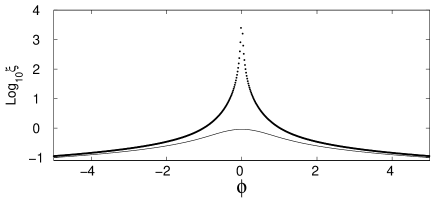
Figure 2: Correlation length $\xi_{C}$ (solid) and of the Entanglement Length $\xi_{E}$ (dotted) for the ground state of the deformed AKLT-Hamiltonians $H(\phi)$ (7).

Let us now develop the mathematical formalism to calculate correlation functions and the LE. We will consider a generalization of the AKLT-states, the family of so–called finitely correlated states (FCS) FNW , which are, in the appropriate limit, dense in the subspace of all translational invariant states. These FCS are completely parameterized by a matrix $A$ as in equations (3,5), but instead of spin–1 systems we consider general spin–$S$ systems. The spin–$1/2$’s are replaced by a spin–$(D-1)/2$, and $|I\rangle$ becomes a maximally entangled state in a $D\times D$ Hilbert space [$A$ is a $(2S+1)\times D^{2}$ matrix; note that $S$ and $D$ are two independent parameters]. These are all unique ground states of gapped local Hamiltonians that can be constructed by calculating the orthogonal complement of an expression equivalent to (2). For simplicity, we will again consider a spin chain with spin $S$ at sites $1\ldots N$ and spin $(D-1)/2$ at the end points. Expectation values of the form $\langle V|\hat{O}_{1}\otimes\hat{O}_{2}\otimes\cdots\hat{O}_{N}|V\rangle$ can readily be calculated by defining the real $D^{2}\times D^{2}$ matrices $R(\hat{O})$ as

$$R_{ij}(\hat{O})=M_{ik}{\rm Tr}\left[(A^{\dagger}\hat{O}A)\sigma_{j}\otimes\sigma_{k}\right]$$ (8)

with $\{\sigma_{\alpha}\}$ a complete orthonormal basis for hermitian operators including $\sigma_{0}=\openone$. The matrix $M$ depends on the choice of $|I\rangle$ and of the basis $\{\sigma_{\alpha}\}$; in the case of the singlet state and $\{\sigma_{\alpha}\}$ the Pauli matrices, $M={\rm diag}[1,-1,-1,-1]$. For the example presented in the previous section, e.g., $R(\hat{\openone})$ is given by

$$R(\openone)=\left(\begin{array}[]{cccc}3\cosh(2\phi)&0&0&\sinh(2\phi)\\ 0&-1&0&0\\ 0&0&-1&0\\ -3\sinh(2\phi)&0&0&-\cosh(2\phi)\\ \end{array}\right).$$

Evaluating expectation values becomes equivalent to calculating the $(0,0)$ element of the matrix product

$$\left[R(\hat{O}_{N})R(\hat{O}_{N-1})\cdots R(\hat{O}_{1})\right]_{(0,0)}.$$

The normalization of $|V\rangle$ is clearly given by $\left[(R(\openone))^{N}\right]_{(0,0)}$, and therefore correlation functions can be calculated as

$$\langle\hat{O}_{1}\otimes\hat{O}_{2}\otimes\cdots\hat{O}_{N}\rangle=\frac{\left[R(\hat{O}_{N})\cdots R(\hat{O}_{1})\right]_{(0,0)}}{\left[(R(\openone))^{N}\right]_{(0,0)}}.$$

To calculate the LE, we need to do an optimization over all possible local bases $\{\beta_{i}\}$ (including overcomplete ones corresponding to generalized measurements). If one measures all spins $k=1\ldots N$ in the basis $\{|\beta_{k}\rangle\}$, the state of the two extremal spins is conditioned on the outcomes $\{\beta_{1},\ldots,\beta_{N}\}$ and given by

$$|\psi_{\beta_{1},\ldots,\beta_{N}}\rangle=\left(\openone\otimes A^{\beta_{N}}\cdots A^{\beta_{1}}\right)|I_{\bar{0},N+1}\rangle,$$ (9)

where we used the notation $\langle\beta_{i}|A=\langle I|A^{\beta_{i}}\otimes\openone$. The probability for this outcome to happen is

$$p_{\beta_{1},\ldots,\beta_{N}}=\frac{\langle\psi_{\beta_{1},\ldots,\beta_{N}}|\psi_{\beta_{1},\ldots,\beta_{N}}\rangle}{\langle V|V\rangle}.$$

Following VDD03 , a generalization of the concurrence Wootters for pure bipartite $D\times D$ states is given by $C(|\chi\rangle=B\otimes\openone_{D}|I\rangle)=|det(B)|^{2/D}/\langle\chi|\chi\rangle$. Using this measure, the average entanglement factorizes and is given by

$$\frac{\sum_{\beta_{1},\ldots,\beta_{N}}|\det(A^{\beta_{N}}\cdots A^{\beta_{1}})|^{\frac{2}{D}}}{\langle V|V\rangle}=\frac{\prod_{i}\left(\sum_{\beta_{i}}|\det(A^{\beta_{i}})|^{\frac{2}{D}}\right)}{\langle V|V\rangle}$$

Obviously, the optimal strategy is to measure all spins in the same basis that maximizes $\sum_{\beta_{i}}|\det(A^{\beta_{i}})|^{\frac{2}{D}}$. This problem is equivalent to calculating the entanglement of assistance (EoA) EoA of the (unnormalized) $D^{2}\times D^{2}$ state $A^{\dagger}A$, and can in general easily be done numerically.

In the case of singlet valence bonds ($D=2$) and $A$ an arbitrary $3\times 4$ matrix, this EoA can be calculated exactly laustsen . Making use of the results in lorsvd , one obtains the exact expression for the LE:

$$E_{\bar{0},N+1}=\frac{\left[\sqrt{\lambda_{\max}(MR(\openone)M(R(\openone))^{T})}\right]^{N}}{\left[(R(\openone))^{N}\right]_{00}}.$$ (10)

Here $R(\openone)$ was defined in (8), $M={\rm diag}[1,-1,-1,-1]$, and $\lambda_{\max}$ means the largest eigenvalue.

Let us investigate the general conditions under which the entanglement length as defined by the LE (10) diverges. It can be shown Popp that this will happen if and only if there exists an operator $Q$ such that the EoA of $(Q^{\dagger}\otimes Q^{\dagger})A^{\dagger}A(Q\otimes Q)$ is maximal, i.e. when it can be written as a convex combination of maximally entangled states (such as for the AKLT); this is indeed the necessary and sufficient condition for perfect entanglement swapping to be possible. Let us compare this with the condition for the presence of a generalized string order parameter, which we define as in (6) but with an extra optimization over the hermitian operator $X$ in $\otimes_{k}\exp(i\pi X_{k})$ instead of $S_{z}$. The condition is now the existence of an operator $Q$ such that $(Q^{\dagger}\otimes Q^{\dagger})A^{\dagger}A(Q\otimes Q)$ is diagonal in a basis of maximally entangled states that have either support in the $|01\rangle\pm|10\rangle$ or in the $|00\rangle\pm|11\rangle$ subspace; this gives two extra nontrivial constraints as compared to the condition for a diverging entanglement length, and hence there exist ground states with vanishing string order parameter, but infinite entanglement length.

Let us conclude by discussing some generalizations to the present results. First of all, the formalism developed in this paper allows us to calculate the localizable entanglement for ground states of arbitrary Hamiltonians numerically by making use of the Density Renormalization Group formalism (DMRG) DMRG : the fixed point of the DMRG algorithm yields a FCS Ostlund ; FNW on which we can apply the machinery presented. Secondly, the results presented equally apply to higher dimensional AKLT-models, and reveal an intriguing connection with quantum computation cluster . Finally, we have done numerical diagonalizations of the Heisenberg antiferromagnetic spin-1 Hamiltonian $H=\sum_{k}\vec{S}_{k}\vec{S}_{k+1}$ with spin 1/2’s at the end points Popp . The localizable entanglement between the end points is again $1$ independent of the number of spins $N$ and is obtained by measuring in the optimal basis (4) for the AKLT: the entanglement length in the Heisenberg spin-1 antiferromagnet is also infinite, and hence this ground state could be used as a perfect quantum channel. It is interesting to note that the entanglement length for the spin 1/2 antiferromagnet is also infinite Korepin : the presence of a Haldane-gap severely affects the correlation length, but does not seem to affect the entanglement length.

This work has been supported by the EU IST program (QUPRODIS and RESQ), Kompetenznetzwerk Quanteninformationsverarbeitung der Bayerischen Staatsregierung, SFB631, and DGES under contract BFM2000-1320-C02-01. We thank M. Fannes for useful discussions.

References

- (1) I. Affleck, T. Kennedy, E.H. Lieb and H. Tasaki, Commun. Math. Phys. 115, 477 (1988).
- (2) F.D.M. Haldane, Phys. Lett. 93A, 464 (1983); Phys. Rev. Lett. 50, 1153 (1983).
- (3) F. Verstraete, M. Popp and J.I. Cirac, quant-ph/0307009.
- (4) M. Popp, F. Verstraete and J.I. Cirac, in preparation.
- (5) M. Fannes, B. Nachtergaele and R.F. Werner, Comm. Math. Phys. 144, 443 (1992); Lett. Math. Phys. 25, 249 (1992).
- (6) M. den Nijs and K. Rommelse, Phys. Rev. B 40, 4709 (1989).
- (7) J. Preskill, J. Mod. Opt. 47, 127 (2000).
- (8) C.H. Bennett et al., Phys. Rev. Lett. 70, 1895 (1993).
- (9) M. Zukowski et al., Phys. Rev. Lett. 71, 4287 (1993).
- (10) F. Verstraete, J. Dehaene and B. De Moor, Phys. Rev. A 68, 012103 (2003).
- (11) W.K. Wootters, Phys. Rev. Lett. 80:2245 (1998).
- (12) D. P. DiVincenzo et al. quant-ph/9803033
- (13) T. Laustsen, F. Verstraete and S. J. van Enk, Quant. Inf. and Comp. 3, 64 (2003).
- (14) F. Verstraete, J. Dehaene and B. De Moor, Phys. Rev. A 64, 010101(R) (2001); Phys. Rev. A 65, 032308 (2002).
- (15) S.R. White, Phys. Rev. Lett. 69, 2863 (1992).
- (16) S. Ostlund and S. Rommer, Phys. Rev. Lett. 75, 3537 (1995).
- (17) F. Verstraete and J.I. Cirac, quant-ph/0311130.
- (18) B.-Q. Jin and V.E. Korepin, quant-ph/0309188.