The Uncertainty Relation in “Which-Way” Experiments:
How to Observe Directly the Momentum Transfer using Weak Values

Abstract

A which-way measurement destroys the twin-slit interference pattern. Bohr argued that this can be attributed to the Heisenberg uncertainty relation: distinguishing between two slits a distance $s$ apart gives the particle a random momentum transfer $\wp$ of order $h/s$. This was accepted for more than 60 years, until Scully, Englert and Walther (SEW) proposed a which-way scheme that, they claimed, entailed no momentum transfer. Storey, Tan, Collett and Walls (STCW) on the other hand proved a theorem that, they claimed, showed that Bohr was right. This work reviews and extends a recent proposal [Wiseman, Phys. Lett. A 311, 285 (2003)] to resolve the issue using a weak-valued probability distribution for momentum transfer, $P_{\rm wv}(\wp)$. We show that $P_{\rm wv}(\wp)$ must be nonzero for some $\wp:|\wp|>h/6s$. However, its moments can be identically zero, such as in the experiment proposed by SEW. This is possible because $P_{\rm wv}(\wp)$ is not necessarily positive definite. Nevertheless, it is measurable experimentally in a way understandable to a classical physicist. The new results in this paper include the following. We introduce a new measure of spread for $P_{\rm wv}(\wp)$: half the length of the unit-confidence interval. We conjecture that it is never less than $h/4s$, and find numerically that it is approximately $h/1.59s$ for an idealized version of the SEW scheme with infinitely narrow slits. For this example, the moments of $P_{\rm wv}(\wp)$, and of the momentum distributions, are undefined unless a process of apodization is used. However, we show that by considering successively smoother initial wave functions, successively more moments of both $P_{\rm wv}(\wp)$ and the momentum distributions become defined. For this example the moments of $P_{\rm wv}(\wp)$ are zero, and these moments are equal to the changes in the moments of the momentum distribution. We prove that this relation also holds for schemes in which the moments of $P_{\rm wv}(\wp)$ are non-zero, but it holds only for the first two moments. We also compare these moments to the moments of two other momentum-transfer distributions that have previously been considered, and with the moments of $\hat{p}_{f}-\hat{p}_{i}$ (which is defined in the Heisenberg picture). We find agreement between all of these, but again only for the first two moments. Our results reconcile the seemingly opposing views of SEW and STCW.

I Introduction

I.1 History (to 1995)

In a twin-slit experiment the far field interference pattern is a picture of the transverse momentum distribution $P_{i}(p)$ of the particle, with fringe spacing equal to $h/s$ (see Fig 1(a)).

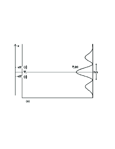
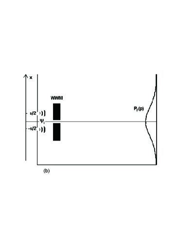
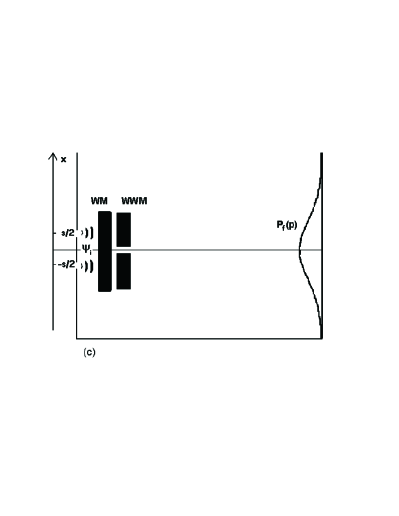
Figure 1: Diagram of a twin-slit which-way experiment. The initial state $|{\psi_{i}}\rangle$ is formed by the slits and propagates longitudinally towards the final screen. This is in the far field, so detecting the position of the particle there is equivalent to measuring its final momentum $p_{f}$. In (a) there is no which-way measurement (WWM) device in place so $p_{f}=p_{i}$, and its distribution is the twin-slit interference pattern. In (b) the WWM device is in place and the distribution for $p_{f}$ is just the single-slit diffraction pattern. In (c), a device is added between the slits and the WWM device which makes a weak measurement (WM) of $|{p_{i}}\rangle\langle{p_{i}}|$, as explained later in the text.

These fringes are a signature of the particle being in a superposition of two positions. Making a position measurement to determine through which slit the particle passed changes the initial momentum distribution to a final distribution $P_{f}(p)$ which lacks such fringes (see Fig. 1(b)). This is the canonical example of Bohr’s complementarity principle BohrEinst ; WheZur83 .

To defend this principle against Einstein’s recoiling slit gedankenexperiment, Bohr relied upon the recently (in 1927) derived Heisenberg uncertainty relation Hei27 to show that the position measurement would cause an “uncontrollable change in the momentum” $\wp\gtrsim h/s$, where $s$ is the slit separation BohrEinst . This is just what is required to wash out the fringes in the momentum distribution, thereby enforcing complementarity. Bohr’s argument was famously reiterated by Feynman FeyLeiSan65 , for a measurement using Heisenberg’s light microscope Hei27 .

Bohr’s argument remained apparently unquestioned until 1991, when Scully, Englert and Walther ScuEngWal91 proposed a new which-way (or welcher Weg) measurement (WWM) for which, they calculated, no momentum would be transferred to the particle. Thus they concluded that the arguments of Feynman and Bohr were wrong in general, and that complementarity must be deeper than uncertainty. Their calculation consisted in showing that a single-slit wavefunction was unchanged by their WWM. This is in contrast to earlier WWMs, such as considered by Feynman and Bohr, which cause an increase in the variance of the single-slit momentum distribution (the diffraction pattern) by of order $(\hbar/s)^{2}$.

Moreover, it can be shown Wis97a that this new feature of the SEW scheme translates into a quantitative difference in the twin-slit pattern. In earlier schemes the variance of the final distribution is greater than that of the initial one, because

$$P_{f}(p)=\int d\wp P_{\rm cl}(\wp)P_{i}(p-\wp).$$ (1)

That is, the momentum disturbance can be treated as a classical mixture of mutually exclusive momentum kicks. The probability distribution $P_{\rm cl}(\wp)$ for transferring momentum $\wp$ is a true (i.e. positive) probability distribution. In the scheme of SEW (and other schemes discussed in Ref. Wis97a ), the relation (1) does not hold. That is, the effect of the SEW WWM is not equivalent to giving the particle a classical momentum kick $\wp$ chosen randomly from a distribution $P_{\rm cl}(\wp)$.

For ‘classical’ WWM schemes, for which Eq. (1) applies, it follows that the differences in the mean and variance of $P_{f}(p)$ and $P_{i}(p)$ are equal to the mean and variance of $P_{\rm cl}(\wp)$. Since the width of $P_{\rm cl}(\wp)$ must be of order $\hbar/s$ to wash out the fringes, it follows that in such cases the variance of $P_{f}(p)$ must be greater than that of $P_{i}(p)$ by of order $(\hbar/s)^{2}$. For nonclassical schemes, such as that of SEW, such a proof does not hold. This difference was first pointed out in Ref. WisHar95 . In particular, for the SEW scheme, the mean and variance of the momentum distribution are unchanged by the WWM Wis97a .

The argument of SEW was not accepted by Storey, Tan, Collett and Walls (STCW) StoTanColWal94 . Since $P_{i}(p)$ has fringes, but $P_{f}(p)$ does not, they reasoned that the momentum must have been disturbed. To back this up, they proved a theorem that showed that if interference is destroyed then there is always some transverse momentum transfer $\geq\hbar/s$. This lower bound of $\hbar/s$ was strengthened in Ref. Wis97a to $\pi\hbar/2s=h/4s$. It was also shown there that the theorem of STCW has the following experimentally verifiable consequence. If the particle were prepared in a momentum eigenstate, with $P_{i}(p)=\delta(p)$, then under any WWM the final momentum distribution would be such that

$$P_{f}(p)\neq 0\textrm{ for some }p\textrm{ such that }|p|>h/4s.$$ (2)

Since Eq. (1) does not always hold, STCW found their momentum transfer not in a probability distribution $P_{\rm cl}(\wp)$, but in a set of probability amplitude distributions $\tilde{O}_{\xi}(\wp)$. The debate QI94 ; Nature95 between SEW and STCW did not lead to any progress in understanding because neither side appeared to appreciate that the other side was using a different concept of momentum transfer. It was only in Ref. WisHar95 that this distinction was clearly made, so that it could be seen that each side had a valid point of view.

I.2 Concepts of Momentum Transfer

The reader might be forgiven for wondering why there is such difficulty with the simple-sounding concept of momentum transfer. Classically, one would just measure the initial momentum $p_{i}$ (just after the slits) and then the final momentum $p_{f}$ (after the WWM), and determine the distribution for $\wp\equiv p_{f}-p_{i}$. The problem with this procedure quantally is that measuring $\hat{p}_{i}$ precisely destroys the twin-slit wavefunction — it creates a momentum eigenstate.

If one were to follow this procedure then one would find that $\wp=p_{f}-p_{i}$ has the same distribution considered above in the context of the argument of STCW. That is, one would find that the absolute value of the momentum transfer $\wp$ would sometimes be larger than $h/4s$. For cases of classical momentum kicks, the distribution for $\wp$ is precisely the $P_{\rm cl}(\wp)$ in Eq. (1), but even in nonclassical cases the width of the distribution must be larger than $h/4s$.

On the other hand, one could well argue that the effect of the WWM on a momentum eigenstate (which is spread over all position) is not the same as its effect on the twin-slit wavefunction. But since this is disturbed by a momentum measurement, one seems restricted to considering the change in the momentum distribution from $P_{i}(p)$ before (or without) the WWM to $P_{f}(p)$ after (or with) the WWM. These are clearly different (the latter lacks fringes), but in terms of the moments, one would find the result quoted above in the context of the argument of SEW. That is, one would find that the mean and variance of the two distributions are identical for the SEW scheme.

One could simply accept that there are two concepts of momentum transfer, and they cannot be reconciled in general. However, it is tempting to try to find a formalism which can get around the above-mentioned problem of the disturbance induced by a measurement of $p_{i}$. What is required is a quantum formalism which somehow treats $p_{i}$ as being definite even when it is not known via a precise measurement.

Two such formalisms have been investigated in the past by one of us and co-workers. The first is the Wigner function Wis97a . The second is Bohmian mechanics Wis98a . Unlike the original works by SEW and STCW, each of these formalisms completely characterizes the momentum transfer $\wp$ by giving a distribution for it. In each case this distribution also depends upon another variable, the transverse position of the particle in the Wigner case, and the time (or longitudinal position) after passing through the WWM in the Bohmian case. Interestingly, in each case the distributions reflect both the results of SEW and of STCW. The interested reader is referred to the original works and the comparison in Ref. Wis03 .

The main drawback of these formalisms is that they are too formal. That is, there is no way to observe directly the distributions of momentum transfer they generate. By ‘to observe directly’ we mean to obtain these distributions from an experiment in a way that would be completely understandable to a classical physicist.

This is the motivation for the current approach, first introduced in Ref. Wis03 , of using the weak value theory of Aharanov, Albert, and Vaidman AhaAlbVai88 . In a nutshell, the idea is to obtain information about the initial momentum by making a weak measurement, so as to disturb the initial wavefunction only negligibly. As will be shown, this approach enables one to observe directly a weak-valued probability distribution $P_{\rm wv}(\wp)$ for momentum transfer $\wp$. Moreover, this distribution reflects both the position of SEW and that of STCW. This surely is the best resolution of the debate that could possibly be hoped for.

I.3 Organization of this Paper

The remainder of this paper is organized as follows. In Sec. II we summarize the theory of weak values as introduced by Aharonov, Albert and Vaidman, and motivate their application to the current issue. In Sec. III we review the formal description of WWMs. Note that we do this in a way different from that adopted previously, including in Ref. Wis03 , in order to integrate weak values into the theory in a more natural way. In Sec. IV we do just that, deriving the expression for $P_{\rm wv}(\wp)$ more elegantly than in Ref. Wis03 .

In Sec. V we expand upon the (very brief) derivations in Wis03 of the elementary properties of $P_{\rm wv}(\wp)$ which show how it is compatible with both SEW and STCW. In Sec. VI we illustrate the properties of $P_{\rm wv}(\wp)$ using a number of different examples. For the simplest conceivable measurement, we calculate $P_{\rm wv}(\wp)$ for a number of different initial states. We also show that the moments of $P_{\rm wv}(\wp)$ (when they are defined) are equal to zero, and equal to the change in the moments from the initial $P_{i}(p)$ to the final $P_{f}(p)$ momentum distributions of the particle. In Sec. VII we calculate the first three moments of the momentum transfer distributions with general WWMs for a number of different momentum-transfer formalisms and show that in general the first and second moments of all of these distributions is equal to the change in the moments of $P_{f}(p)$ and $P_{i}(p)$. However this relationship ceases to hold for higher order moments for all of these formalisms. We conclude in Sec. VIII.

II Weak Values

II.1 Introduction

It is a fundamental fact of quantum theory that a projective measurement, which one could also call a precise or strong measurement, greatly disturbs the quantum state in general. However one can consider imprecise measurements (which are non-projective), for which the disturbance can be small. (The disturbance is not necessarily small because the imprecision may be due simply to poor control of classical noise). A weak measurement of a quantity is one which is arbitrarily imprecise, and for which the disturbance is correspondingly arbitrarily small.

A weak value is just the mean value of a weak measurement. That is, it is obtained by averaging over a large ensemble of weak measurement results on identically prepared systems, just as is the mean value of a strong measurement. However, because of the imprecision in each weak measurement result, the size of the ensemble must be correspondingly larger than in the case of strong measurements.

Simply considering a prepared state $|{\psi}\rangle$ gives an uninteresting weak value — the same as the strong value for the same quantity:

$$\left\langle{X_{\rm weak}}\right\rangle_{\psi}=\left\langle{X_{\rm strong}}\right\rangle_{\psi}=\langle{\psi}|\hat{X}|{\psi}\rangle.$$ (3)

As realized by Aharonov, Albert, and Vaidman AhaAlbVai88 , to obtain an interesting weak value requires post-selection. That is, the average is calculated from the sub-ensemble where a later strong measurement reveals the state to be $|{\phi}\rangle$.

Allowing for some evolution $\hat{U}$ after the weak measurement, the post-selected weak value turns out to be

$${\phantom{\left\langle{X_{w}}\right\rangle}}_{\phi}\!\left\langle{X_{\rm w}}\right\rangle_{\psi}={\rm Re}\frac{\langle{\phi}|\hat{U}\hat{X}|{\psi}\rangle}{\langle{\phi}|\hat{U}|{\psi}\rangle}.$$ (4)

The interested reader is referred to the appendix for a very brief outline of how this formula may be derived.

This expression is certainly unusual, in that the numerator and denominator are linear in $|{\psi}\rangle$ and $|{\phi}\rangle$ rather than bilinear. This has the consequence that the weak value can lie outside the range of eigenvalues of $\hat{X}$ AhaAlbVai88 . This was soon verified experimentally RitStoHul91 . This of course cannot happen for a strong measurement of $\hat{X}$, for which the post-selected strong value would be

$${\phantom{\left\langle{X_{w}}\right\rangle}}_{\phi}\!\left\langle{X_{\rm s}}\right\rangle_{\psi}=\frac{\sum_{x}\left|{\langle{\phi}|\hat{U}|{x}\rangle}\right|^{2}x\left|{\langle{x}|{\psi}\rangle}\right|^{2}}{\sum_{x^{\prime}}\left|{\langle{\phi}|\hat{U}|{x^{\prime}}\rangle}\right|^{2}\left|{\langle{x^{\prime}}|{\psi}\rangle}\right|^{2}}.$$ (5)

II.2 The Motivation

There are three motivations for considering weak values in the context of momentum transfer in WWMs.

The first is that weak values have a good record for supplying new insight into quantum puzzles. They have been used to define tunneling time in a directly observable manner Ste95 and to resolve Hardy’s paradox Aha01 . With a few simple generalizations, weak values have also been found Wis02a to explain “anticausal” conditional quadrature evolution in a well-known cavity QED experiment FosOroCasCar00 .

The second motivation is more specific. To investigate momentum transfer in WWMs one wants to know $\wp=p_{f}-p_{i}$ without making a strong measurement of $p_{i}$. It is an obvious (in hindsight) idea to make a weak measurement.

Thirdly, weak values will enable experimental investigation of the problem, by direct observation of the momentum transfer. The lack of meaningful predictions that are interesting enough to be tested by experimentalists is, in our opinion, one of the problems with this area of research. We note in passing that the experiment by Rempe and co-workers DurNonRem98 , as interesting and elegant as it was, was not relevant to the debate between SEW and STCW. This is simply because it did not involve a which-way measurement of a particle prepared in a superposition of two positions.

III The WWM formalism

As noted previously, we are concerned with the case where the quantum particle is prepared initially in a state $|{\psi_{i}}\rangle$ which is a superposition of two states that are well-localized in position (that is, at the two slits, centred at $\pm s/2$). It is necessary to restrict the discussion to an interferometer of this kind, where the initial superposition is in transverse position and the free evolution preserves the conjugate quantity (transverse momentum), so that the issue of loss of visibility relates directly to the transverse momentum transfer.

In the WWM the particle is coupled to a meter, whose state we will distinguish from that of the system by using a double ket. For instance, the initial state of the meter is $||{\theta}\rangle\rangle$. The coupling of the system and meter can be described by a unitary operator $\hat{U}_{{}_{\rm WWM}}$. This enables the meter to obtain which-way information and as a consequence also change the momentum distribution of the particle. The which-way information can be obtained by the experimenter by reading out the meter. For simplicity we will assume that this is performed by making a measurement of the meter in a complete orthogonal basis $\{||{\xi}\rangle\rangle\}$. Thus the evolution of the system and meter is as follows:

$$||{\theta}\rangle\rangle|{\psi_{i}}\rangle \to \hat{U}_{{}_{\rm WWM}}||{\theta}\rangle\rangle|{\psi_{i}}\rangle$$ (6)

$$\to ||{\xi}\rangle\rangle\langle\langle{\xi}||\hat{U}_{{}_{\rm WWM}}||{\theta}\rangle\rangle|{\psi_{i}}\rangle\,=\,||{\xi}\rangle\rangle\hat{O}_{\xi}|{\psi_{i}}\rangle.$$ (7)

In Eq. (7), $\hat{O}_{\xi}\equiv\langle\langle{\xi}||\hat{U}_{{}_{\rm WWM}}||{\theta}\rangle\rangle$ is an operator in the system Hilbert space called the measurement operator. The WWM is completely described by the set of measurement operators $\{\hat{O}_{\xi}\}$. The probability to obtain the result $\xi$ is $\langle{\psi_{i}}|\hat{O}_{\xi}^{\dagger}\hat{O}_{\xi}|{\psi_{i}}\rangle$. The final state in Eq. (7) must be divided by the square root of this in order for it to be normalized.

For a WWM we need to obtain information about the position of the particle. That means that we want the measurement operators to be functions of the position operator: $\hat{O}_{\xi}=O_{\xi}(\hat{x})$. Thus the WWM is described by the set of functions $\left\{{O_{\xi}(x)}\right\}$, which are restricted only by the completeness relation

$$\sum_{\xi}|O_{\xi}(x)|^{2}=1\;\forall x.$$ (8)

This is necessary for the probabilities of the results $\xi$ to sum to unity.

For some WWMs, the read-out basis $||{\xi}\rangle\rangle$ can be chosen such that ${O}_{\xi}(\hat{x})=\sqrt{N_{\xi}}\exp(-ik_{\xi}\hat{x})$ for all $\xi$, where obviously $\sum_{\xi}N_{\xi}=1$. In such cases Eq. (1) can be shown to pertain WisHar95 ; Wis97a , where

$$P_{\rm cl}(\wp)=\sum_{\xi}N_{\xi}\delta(\wp-\hbar k_{\xi})$$ (9)

That is, $N_{\xi}$ can be interpreted as the probability for the system to receive a momentum kick equal to $\hbar k_{\xi}$.

In general, Eq. (1) does not pertain, but an analogous equation for probability amplitudes does,

$$\langle{p}|\hat{O}_{\xi}|{\psi_{i}}\rangle=\int\!d\wp\,\tilde{O}_{\xi}(\wp)\tilde{\psi}_{i}(p-\wp).$$ (10)

Here,

$$\tilde{O}_{\xi}(p)=(2\pi\hbar)^{-1/2}\int\!dx\,O_{\xi}(x)e^{-ixp/\hbar}$$ (11)

is the probability amplitude for a momentum kick $\wp$, as identified by STCWStoTanColWal94 and similarly

$$\tilde{\psi}_{i}(p)=(2\pi\hbar)^{-1/2}\int\!dx\,\psi_{i}(x)e^{-ixp/\hbar},$$ (12)

where $\psi_{i}(x)=\langle{x}|{\psi_{i}}\rangle$.

For narrow slits, [i.e. $|\psi(x)|^{2}\simeq\delta(2x+s)+\delta(2x-s)$], the visibility of the far field interference pattern can be shown Wis97a to be given by

$$V=\left|{\sum_{\xi}O_{\xi}(-s/2)O_{\xi}^{*}(s/2)}\right|.$$ (13)

From this and Eq. (10), it can be shown Wis97a that the WWM will disturb a momentum eigenstate by an amount at least equal to $\arccos(V)\hbar/s$. For $V=0$ one obtains the previously stated lower bound, $h/4s$. Since the visibility is only defined for a twin-slit wavefunction, the disturbance to a momentum eigenstate actually reflects the quality of the WWM (which exists independently of the visibility of the fringe pattern). This quantity, $Q$, is defined and analysed in Ref. MarHar03 .

IV Applying Weak Values to WWMs

Clearly to apply weak values to WWMs it is necessary to make the weak measurement on $|{\psi_{i}}\rangle$ before the WWM, followed by a strong measurement of $\hat{p}$ (which is simply a measurement of position in the far-field), as shown in Fig. 1(c).

A first thought would be to make a weak measurement of $\hat{p}$. Including the initial meter state and the final meter state (for a particular result $\xi$), and describing the WWM by the unitary operator $\hat{U}_{{}_{\rm WWM}}$, one can apply Eq. (4). This yields the weak value

$${\phantom{\left\langle{X_{w}}\right\rangle}}_{p_{f},\xi}\!\left\langle{p_{\rm w}}\right\rangle_{\theta,\psi_{i}}={\rm Re}\frac{\langle{p_{f}}|\langle\langle{\xi}||\hat{U}_{{}_{\rm WWM}}\hat{p}\,||{\theta}\rangle\rangle|{\psi_{i}}\rangle}{\langle{p_{f}}|\langle\langle{\xi}||\hat{U}_{{}_{\rm WWM}}||{\theta}\rangle\rangle|{\psi_{i}}\rangle}.$$ (14)

That is, one could measure the weak value of the initial momentum $p_{i}$, post-selected on the final momentum $p_{f}$ and WWM result $\xi$.

A little consideration of Eq. (14) reveals that this is not what we want. Say it turned out that the weak value of the initial momentum was the same as the final momentum: ${\phantom{\left\langle{X_{w}}\right\rangle}}_{p_{f},\xi}\!\left\langle{\hat{p}_{w}}\right\rangle_{\theta,\psi_{i}}=p_{f}$. Then all that one could say would be that the WWM (for result $\xi$) does not change the mean momentum. This will be the case for any symmetric disturbance of the momentum. To address the momentum transfer issue we need to know of any disturbance to the momentum.

A second (and better) thought is to make a weak measurement of the projector $\hat{\pi}(p_{i})\equiv|{p_{i}}\rangle\langle{p_{i}}|$ for some particular $p_{i}$. The non-post-selected mean value of a measurement (weak or strong) of $\hat{\pi}(p_{i})$ on $|{\psi_{i}}\rangle$ would give the probability $P_{i}(p_{i})=\langle{\psi_{i}}|{p_{i}}\rangle\!\langle{p_{i}}|{\psi_{i}}\rangle$. The post-selected weak value

$${\phantom{\left\langle{X_{w}}\right\rangle}}_{\xi,p_{f}}\!\left\langle{\pi(p_{i})_{\rm w}}\right\rangle_{\theta,\psi_{i}}={\rm Re}\frac{\langle{p_{f}}|\langle\langle{\xi}||\hat{U}_{{}_{\rm WWM}}\hat{\pi}(p_{i})\,||{\theta}\rangle\rangle|{\psi_{i}}\rangle}{\langle{p_{f}}|\langle\langle{\xi}||\hat{U}_{{}_{\rm WWM}}||{\theta}\rangle\rangle|{\psi_{i}}\rangle}$$ (15)

can thus be interpreted as the weak-valued conditional probability for the initial momentum being $p_{i}$, given $p_{f}$ and $\xi$. We will denote this $P_{\rm wv}(p_{i}|\xi,p_{f})$.

Using this expression for $P_{\rm wv}(p_{i}|\xi,p_{f})$, we can define a weak-valued joint probability distribution

$$P_{\rm wv}(p_{i};\xi,p_{f})=P_{\rm wv}(p_{i}|\xi,p_{f})\times P(\xi,p_{f}),$$ (16)

where

$$P(\xi,p_{f})=\left|{\langle{p_{f}}|\langle\langle{\xi}||\hat{U}_{{}_{\rm WWM}}||{\theta}\rangle\rangle|{\psi_{i}}\rangle}\right|^{2}$$ (17)

is the probability to obtain the result $\xi$ and the final momentum $p_{f}$.

We are now almost at our goal of quantifying the momentum transfer $\wp=p_{f}-p_{i}$. We rewrite $P_{\rm wv}(p_{i};\xi,p_{f})$ in terms of $\wp$, $p_{i}$, and $\xi$, and then average over all $p_{i}$, and over all results $\xi$. This means repeating the experiment many times for all choices of $p_{i}$. The result is the weak-valued probability distribution for the momentum transfer $\wp$,

$$P_{\rm wv}(\wp)\equiv\sum_{\xi}\int dp_{i}P_{\rm wv}(p_{i};\xi,p_{i}+\wp)$$ (18)

Using Eqs. (15)–(17) and the definition of $\hat{O}_{\xi}$, one finds that $P_{\rm wv}(\wp)$ is equal to

$$\sum_{\xi}\int\!dp_{i}\,{\rm Re}\left\{{\langle{p_{i}+\wp}|\hat{O}_{\xi}|{p_{i}}\rangle\langle{p_{i}}|{\psi_{i}}\rangle\langle{\psi_{i}}|\hat{O}_{\xi}^{\dagger}|{p_{i}+\wp}\rangle}\right\}.$$ (19)

Finally, using $\hat{O}_{\xi}=O_{\xi}(\hat{x})$, one can straightforwardly derive the remarkably simple and elegant formula

$$P_{\rm wv}(\wp)=\sum_{\xi}{\rm Re}\left\{{\tilde{O}_{\xi}(\wp)\tilde{Q}_{\xi}^{*}(\wp)}\right\}.$$ (20)

The Fourier transform is as defined in Eq. (11), and

$$Q_{\xi}(x)=O_{\xi}(x)|\psi_{i}(x)|^{2}.$$ (21)

Thus the weak-valued probability distribution for $\wp$ depends upon the initial state in a very natural way.

V Elementary Properties of $P_{\rm wv}(\wp)$

V.1 Proofs

A number of interesting properties of $P_{\rm wv}(\wp)$ can now easily be proven.

First, $P_{\rm wv}(\wp)$ is normalized. This is easily seen using the moment-generating function

$$\Phi(q) \equiv \int\!d\wp\,P_{\rm wv}(\wp)e^{i\wp q/\hbar}$$ (23)

$$= \sum_{\xi}\int\!dx\,|\psi_{i}(x)|^{2}\mbox{$\frac{1}{2}$}\bigl{[}O_{\xi}(x)O_{\xi}^{*}(x-q)$$

$${\phantom{\sum_{\xi}\int\!dx\,}+}\,O_{\xi}^{*}(x)O_{\xi}(x+q)\bigr{]}.$$

Note that this expression [and Eq. (29)] correct a mistake in Ref. Wis03 which did not affect the results stated there. As we will see later, $P_{\rm wv}(\wp)$ may take negative values, but it integrates to

$$\Phi(0)=\int dx\sum_{\xi}|O_{\xi}(x)|^{2}|\psi_{i}(x)|^{2}=\int dx|\psi_{i}(x)|^{2}=1.$$ (24)

Moreover, from Eq. (23) it can be shown that $|\Phi(q)|\leq 1$, as it would be for a true probability distribution. This is the case as

$$|\Phi(q)| \leq \sum_{\xi}\int dx\frac{1}{2}\left.|O_{\xi}^{*}(x-q)O_{\xi}(x)\right.$$

$$\phantom{\sum_{\xi}\int dx\frac{1}{2}}\left.+O_{\xi}^{*}(x)O_{\xi}(x+q)|\,|\psi_{i}(x)|^{2}\right.$$

$$\leq \sum_{\xi}\int dx\frac{1}{2}\left.\bigl{[}|O_{\xi}^{*}(x-q)O_{\xi}(x)|\right.$$

$$\phantom{\sum_{\xi}\int dx\frac{1}{2}}\left.+|O_{\xi}^{*}(x)O_{\xi}(x+q)|\bigr{]}\,|\psi_{i}(x)|^{2},\right.$$

which follows from the triangle inequality. Using the Schwarz inequality we obtain

$$|\Phi(q)| \leq \sum_{\xi}\int dx\frac{1}{2}\left.\bigl{[}|O_{\xi}(x-q)||O_{\xi}(x)|\right.$$ (26)

$$\phantom{\sum_{\xi}\int dx\frac{1}{2}}\left.+|O_{\xi}(x)||O_{\xi}(x+q)|\bigr{]}|\psi_{i}(x)|^{2}\right.$$

$$\leq \sum_{\xi}\int dx\frac{1}{4}\left.\bigl{[}|O_{\xi}(x-q)|^{2}+2|O_{\xi}(x)|^{2}\right.$$

$$\phantom{\sum_{\xi}\int dx\frac{1}{2}}\left.+|O_{\xi}(x+q)|^{2}\bigr{]}|\psi_{i}(x)|^{2},\right.$$

where the last line follows from the fact that $(|A|-|B|)^{2}\geq 0$. Using the completeness relation from Eq. (8), then, we have achieved $|\Phi(q)|\leq 1$, as desired.

Second, in the case of a classical momentum disturbance (9), it is easy to see that

$$P_{\rm wv}(\wp)=P_{\rm cl}(\wp),$$ (27)

which is a true probability distribution. This is an important test-case. It shows that if $P_{\rm wv}(\wp)$ takes negative values for some WWM scheme, that scheme must involve a nonclassical momentum disturbance. As a special case, if there is no WWM at all, $P_{\rm wv}(\wp)=\delta(\wp)$, indicating that there is no momentum disturbance, as expected.

Third, since the moments of $\wp$ are given by

$$\left\langle{\wp^{n}}\right\rangle_{\rm wv}=\left({-i\hbar{\partial}/{\partial{q}}}\right)^{n}\Phi(q)|_{q=0},$$ (28)

it follows from Eq. (23) that if the $O_{\xi}$ are flat (i.e. have all derivatives zero) in the region of the slits where $|\psi_{i}(x)|^{2}$ is nonzero, then all of the moments of $P_{\rm{wv}}(\wp)$ are zero. This is the case (to a very good approximation) in the scheme of SEW. Thus the claim that their scheme would not transfer any momentum to the particle could be validated experimentally by calculating the moments of the measured $P_{\rm wv}(\wp)$.

Fourth and finally, despite this last fact, $P_{\rm wv}(\wp)$ also reflects the change in the momentum distribution caused by a WWM, as we now show. For narrow slits at $x=\pm s/2$,

$$\Phi(s)=\frac{1}{4}\left[{\cal V}\left(\frac{3s}{2},\frac{s}{2}\right)+2{\cal V}\left(\frac{s}{2},\frac{-s}{2}\right)+{\cal V}\left(\frac{-s}{2},\frac{-3s}{2}\right)\right],$$ (29)

where

$${\cal V}(x,x^{\prime})\equiv\sum_{\xi}O_{\xi}(x)O_{\xi}^{*}(x^{\prime}).$$ (30)

From Eq. (13), the visibility $V$ of the interference pattern is $|{\cal V}(\frac{s}{2},\frac{-s}{2})|$. With a WWM in place, this will be zero. Hence, by the triangle inequality, we have

$$|\Phi(s)| \leq \frac{1}{4}\left[{\left|{{\cal V}\left({\frac{3s}{2},\frac{s}{2}}\right)}\right|+\left|{{\cal V}\left({\frac{-s}{2},\frac{-3s}{2})}\right)}\right|}\right]$$ (31)

$$\leq \frac{1}{2}.$$

Here we have used $|{\cal V}(x,x^{\prime})|\leq 1$, which follows from the definition in Eq. (30). Since in addition $\Phi(0)=1$ and $|\Phi(q)|\leq 1\;\forall q$, it follows from the theorem in Appendix A of Ref. Wis97a that

$${\rm Support}[P_{\rm wv}(\wp)]\not\subset(-h/6s,h/6s).$$ (32)

That is, $P_{\rm wv}(\wp)$ must be nonzero for some $\wp$ having a magnitude at least equal to $h/6s$. This supports the view of STCW. For an imperfect WWM where $V\neq 0$, $h/6s$ must be replaced by $(\hbar/s)\arccos[(V+1)/2]$ fn1 .

V.2 Conjectures

In Ref. Wis97a a similar lower bound to that in Eq. (32) was proven for (a) the final momentum distribution where the system had been prepared in the zero-momentum eigenstate, and (b) the “nonlocal” momentum transfer function in the Wigner representation. In these cases, the lower bound was greater: $h/4s$ rather than $h/6s$. Also, in these cases, the lower bound could be achieved by using a classical momentum disturbance with

$$P_{\rm cl}(\wp)=\frac{1}{2}\left[\delta\left({\wp+\frac{h}{4s}}\right)+\delta\left({\wp-\frac{h}{4s}}\right)\right].$$ (33)

Because of the similarity of the analysis in the cases of Ref. Wis97a and the weak-valued momentum transfer probability distribution here, we conjecture that the lower bound of $h/6s$ in Eq. (32) cannot be achieved. Rather, we conjecture, that the achievable lower bound is $h/4s$, and that it is achieved for $P_{\rm wv}(\wp)=P_{\rm cl}(\wp)$ in Eq. (33).

Although the measure

$$[\delta\wp]_{\rm support}={\rm min}\left\{{p:\;{\rm Support}[P_{\rm wv}(\wp)]\subset(-p,p)}\right\}$$ (34)

is useful in that we can prove a lower bound of $h/6s$ and conjecture a lower bound of $h/4s$, its disadvantage as a measure of the width of $P_{\rm wv}(\wp)$ is that for nonclassical measurements it is typically infinite, as we will see in Sec. VI. For classical distributions, this measure is the same as the $\infty$-norm of the distribution, where the $n$-norm is defined as

$$[\delta\wp]_{n-{\rm norm}}=\left[{\int d\wp P_{\rm cl}(\wp)|\wp|^{n}}\right]^{1/n}.$$ (35)

However, in general this may be undefined even for $n=1$, unless the distribution is apodized, as discussed in Sec. VI.1.

For classical distributions, $[\delta\wp]_{\infty-{\rm norm}}$ is also equivalent to the unit-confidence interval width, $[\delta\wp]_{1-{\rm confidence}}$, where

$$[\delta\wp]_{\epsilon-{\rm confidence}}=p:\int_{-p}^{p}P_{\rm wv}(\wp)d\wp=\epsilon$$ (36)

For non-positive distributions this definition still applies, with a slight modification:

$$[\delta\wp]_{\epsilon-{\rm confidence}}={\rm min}\left\{{p:\int_{-p}^{p}P_{\rm wv}(\wp)d\wp=\epsilon}\right\}$$ (37)

The interesting point with non-positive distributions is that $[\delta\wp]_{1-{\rm confidence}}$ may be finite, even if $[\delta\wp]_{\rm support}$ is infinite.

We will see that $[\delta\wp]_{1-{\rm confidence}}$ is a good measure of the width for the very nonclassical $P_{\rm wv}(\wp)$ in Sec. VI.1. Moreover, it evaluates to a quantity of order, but larger than $h/4s$. On this basis, we conjecture, as we did for $[\delta\wp]_{\rm support}$, that this measure satisfies

$$[\delta\wp]_{1-{\rm confidence}}\geq\frac{h}{4s},$$ (38)

and that the lower bound is met only for the classical distribution (33).

VI Examples

The results of the previous section can be illustrated by a number of examples with different initial wavefunctions $\psi_{i}(x)$. These examples all use a minimal WWM that only distinguishes between $x<0$ and $x>0$. That is, $O_{\pm}(x)=\Theta(\pm{x})$, the Heaviside function. This is an idealization of the WWM of SEW. In this instance, of course $O_{\pm}(x)$ are perfectly flat in the region of the slits, so from the above arguments all moments should vanish in each of these cases.

The simplest example of infinitely narrow slits considered in Wis03 proves to have difficulty in showing some of the nice properties of $P_{\rm{wv}}(\wp)$. This is because all moments above zero order are undefined in a strict sense. The theory of apodization Zema is required in order to give the “correct” moments in this case. For better behaved initial states, however, this becomes less of a problem, as we shall see. For an arbitrarily smooth initial state, arbitrarily many moments vanish without the need for an apodizing function. For all of these examples, however, Eq. (32) still holds. This is possible because in all of these examples $P_{\rm{wv}}(\wp)$ takes on negative values. That is, the WWM involves a nonclassical momentum transfer.

VI.1 Unbounded $\psi_{i}$

For our first example we consider infinitely narrow slits centered at $\pm s/2$. The minimal which way measurement functions, $\{O_{\pm}(x)\}$, mentioned above are used. Evaluating Eq. (20) then gives

$$P_{\rm{wv}}(\wp)=\frac{1}{2}\bigl{[}\delta(\wp)+\frac{\sin(\wp{s}/2\hbar)}{\pi\wp}\bigr{]}$$ (39)

This distribution is plotted in Figure 2 along with $P_{i}(p)$ and $P_{f}(p)$ for the same initial state and measurement operators.

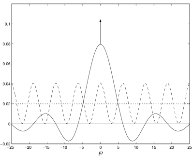
Figure 2: Plots of the weak valued momentum transfer distribution, $P_{\rm{wv}}(\wp)$, along with $P_{i}(p)$ and $P_{f}(p)$ for narrow slits with $s=1$. The solid line corresponds to $P_{\rm{wv}}(\wp)$, the dashed line to $P_{i}(p)$ and the dotted line to $P_{f}(p)$. The arrow denotes half of the delta function. The momentum is scaled by taking $\hbar=1$. It should be noted that both the initial and final momentum distributions are in reality spread out over all space in this case and are thus actually infinitely small. In order to compare them with $P_{\rm{wv}}(\wp)$ they are shown here to be normalized over the interval which they are plotted for.

Obviously this is an example of a non-classical measurement as $P_{\rm{wv}}(\wp)$ takes negative values periodically. All moments of order one and above are undefined in the strict sense. If, however, we multiply by an apodizing function $f_{\kappa}(\wp)$ with characteristic width $\kappa$ that has all its moments defined and smoothly goes to the unit function as $\kappa\to\infty$, then we get the “corrected” moments. A simple example is $f_{\kappa}(\wp)=\exp(-|\wp|/\kappa)$. We take the apodized moments of $P_{\rm{wv}}(\wp)$ to be

$$\langle{\wp^{n}}\rangle_{\rm{wv}} = \lim_{\kappa\to\infty}\int d\wp P_{wv}(\wp)f_{\kappa}(\wp)\wp^{n}$$ (40)

For this example we get

$$\langle{\wp^{n}}\rangle_{\rm{wv}} = \left.\lim_{\kappa\to\infty}\left[\frac{(1+(-1)^{n})\Gamma(n)\sin(n\arctan(\kappa{s}/2\hbar))}{(1/2\kappa)^{n}(4+(\kappa{s}/\hbar)^{2})^{n/2}}\right]\right.$$ (41)

$$= \left.0\,\,\forall{n}\right.$$

Even though the moments of this distribution are identically zero, Eq. (32) for its support is still satisfied. The unit-confidence half-interval is found to be $[\delta\wp]_{1-{\rm confidence}}\approx h/1.59s$. Thus even though the moments of this distribution vanish, Eq. (32) for the support of the distribution is clearly satisfied. The non-zero width of $P_{\rm wv}(\wp)$ can also be seen in its $1$-norm, as defined in Eq. (35). For this case it is necessary to use an apodization function to calculate it. We find that $[\delta\wp]_{1-{\rm norm}}=2h/\pi{s}$, which is again greater than $h/4s$.

VI.2 Bounded $\psi_{i}$

We now consider another example, which is more realistic. Consider the case of rectangular slits of width $w$ centered at $\pm s/2$. We can write the wave function for this case as

$$\psi_{i}(x) = \left.\frac{1}{\sqrt{2w}}\Theta(x+w/2)\Theta(-x+w/2)\ast(\delta(x+s/2)\right.$$ (42)

$$\phantom{\frac{1}{\sqrt{2w}}}\left.+\delta(x-s/2)),\right.$$

where $f\ast g$ denotes the convolution of $f$ with $g$. In this case we find that

$$P_{\rm{wv}}(\wp)=\frac{1}{2}[\delta(\wp)+\frac{2}{\pi w\wp^{2}}\sin(\wp{s}/2\hbar)\sin(\wp{w}/2\hbar)].$$ (43)

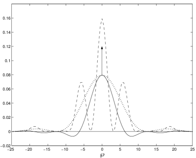
Figure 3: Plots of the weak valued momentum transfer distribution, $P_{\rm{wv}}(\wp)$, along with $P_{i}(p)$ and $P_{f}(p)$ for rectangular slits with width $w=1/2$. Other details are as in Fig. 2, but note that here $P_{i}$ and $P_{f}$ are correctly normalized.

This distribution is plotted in Figure 3 along with $P_{i}(p)$ and $P_{f}(p)$. This distribution obviously has its first moment defined without need for apodization. Second and higher order moments, however, remain undefined in the strict sense.

VI.3 Continuous $\psi_{i}$

For our next example, we consider a bounded and continuous initial state. Specifically,

$$\psi_{i}(x) = \left.\frac{1}{\sqrt{w}}\cos(\frac{\pi}{w}x)\Theta(x+w/2)\Theta(-x+w/2)\right.$$ (44)

$$\phantom{\frac{1}{\sqrt{w}}}\left.\ast(\delta(x+s/2)+\delta(x-s/2)).\right.$$

Given this initial state and the minimal WWM, we find that

$$P_{\rm{wv}}(\wp) = \frac{1}{2}\left[\delta(\wp)-\frac{\sin(\wp{s}/2\hbar)}{\hbar{w}\wp}\left(\frac{\sin(\frac{w}{2\hbar}(\wp-\frac{\pi\hbar}{w}))}{\wp-\frac{\pi\hbar}{w}}\right.\right.$$

$$\phantom{\frac{1}{2}[}\left.\left.+\,\frac{\sin(\frac{w}{2\hbar}(\wp+\frac{\pi\hbar}{w}))}{\wp+\frac{\pi\hbar}{w}}\right)\right]$$

$$= \frac{1}{2}\left[\delta(\wp)-\frac{2\pi\sin(\wp{s}/2\hbar)\cos(\wp{w}/2\hbar)}{(\hbar{w}\wp)[\wp^{2}-(\pi\hbar/w)^{2}]}\right].$$

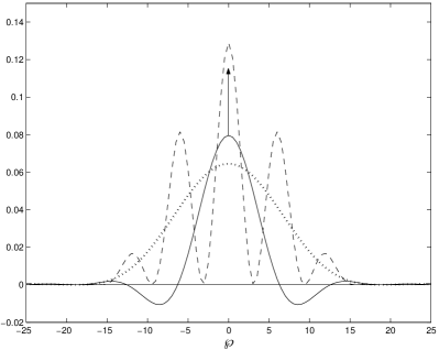
Figure 4: Plots of the weak valued momentum transfer distribution, $P_{\rm{wv}}(\wp)$, along with $P_{i}(p)$ and $P_{f}(p)$ for the continuous initial wave function defined in Sec. VI C. Other details are as in Fig. 3.

This distribution is plotted in Figure 4 along with $P_{i}(p)$ and $P_{f}(p)$. This distribution has both its first and second moments defined without need for apodization. They vanish, of course. The theory of apodization is still required, however, to obtain the correct higher order moments.

VI.4 Smooth $\psi_{i}$

In the previous sections we found that more moments become defined without the need for an apodizing function as we consider smoother initial states. We will now consider what happens as our initial state becomes differentiable to higher and higher order. That is, we shall consider the case of

$$\psi_{i}(x) = \left.\frac{1}{\sqrt{N}}\cos^{n}\left(\frac{\pi}{w}x\right)\Theta(x+w/2)\Theta(-x+w/2)\right.$$ (47)

$$\phantom{\frac{1}{\sqrt{w}}}\left.\ast(\delta(x+s/2)+\delta(x-s/2)),\right.$$

where

$$N=\frac{4w}{\sqrt{\pi}}\frac{\Gamma(1/2+n)}{\Gamma(1+n)}.$$

Note that the previous two examples are special cases of this, corresponding to $n=0$ for Sec. VI C and $n=1$ for Sec. VI D. By considering this general case we will be able to make our initial state arbitrarily smooth by considering arbitrary degrees of $n$. For the case of general $n$ we find

$$P_{\rm{wv}}(\wp) = \frac{1}{2}\left[\delta(\wp)+\frac{1}{2^{n+1}\wp}\sin(\wp{s}/2\hbar)\sum_{k=0}^{n}{n\choose k}\right.$$ (48)

$$\phantom{\frac{1}{2}[}\left.\times\frac{\sin(\frac{w}{2\hbar}(\wp-\frac{(n-2k)\hbar\pi}{w})}{\wp-\frac{(n-2k)\hbar\pi}{w}}\right].$$

For the case of even $n$ this simplifies to

$$P_{\rm{wv}}(\wp) = \frac{1}{2}\left[\delta(\wp)+\frac{n!}{2}\left(\frac{\pi\hbar}{w}\right)^{n}(-1)^{n/2}\right.$$

$$\left.\times\frac{\sin(\wp{s}/2\hbar)\sin(\wp{w}/2\hbar)}{(\wp-\frac{n\hbar\pi}{2})(\wp-\frac{(n-2)\hbar\pi}{2})\ldots(\wp+\frac{n\hbar\pi}{2})}\right].$$

For odd $n$ it becomes

$$P_{\rm{wv}}(\wp) = \frac{1}{2}\left[\delta(\wp)+\frac{n!}{2}\left(\frac{\hbar\pi}{w}\right)^{n}(-1)^{(n+1)/2}\right.$$

$$\left.\times\frac{\sin(\wp{s}/2\hbar)\cos(\wp{w}/2\hbar)}{(\wp-\frac{n\hbar\pi}{2})(\wp-\frac{(n-2)\hbar\pi}{2})\ldots(\wp+\frac{n\hbar\pi}{2})}\right].$$

From Eq. (VI.4) and Eq. (VI.4), for an initial state like the cosine function raised to the power of $n$, it is easy to see that $n+1$ moments are defined without the need for an apodizing function. Thus as the initial state becomes smoother and smoother arbitrarily many moments become defined without apodization. Furthermore, all moments that are defined will be zero where the measurement functions $O_{\xi}(x)$ are flat in the region of the slits.

VII Moments of $P_{\rm wv}(\wp)$ and other distributions

In the preceding section we showed that in twin-slit schemes where the measurement functions $O_{\xi}(x)$ are flat in the region of the slits, all of the moments of $P_{\rm{wv}}(\wp)$ are zero. As discussed in the introduction, these types of WWMs have no effect on single slit diffraction patterns. As such, the mean and variance of a twin-slit diffraction pattern are not affected by such a measurement. Obviously then, the first and second moments of $P_{\rm wv}(\wp)$ are equal to the change in the moments for the momentum distribution of the particle. In this section we show that this is true for all WWMs, provided that the measurement functions $O_{\xi}(x)$ vary slowly on the scale of the slits. However, the third moment of $P_{\rm wv}(\wp)$ does not correspond in general to the difference in the third moments of the final and initial momentum distributions of the particle. We show that this apparent discrepancy also arises from all known formalisms investigating momentum transfer in WWMs (including a new one introduced here). Moreover, with one exception, all of these third moments are different.

VII.1 Moments of $P_{\rm wv}(\wp)$

The moments of the weak valued momentum transfer probability distribution, $P_{\rm{wv}}(\wp)$, can most easily be calculated using the characteristic function of Eq. (23). The $n^{\rm{th}}$ moment of this distribution is

$$\langle\wp^{n}\rangle_{\rm{wv}} = \left.\left(-i\hbar\frac{\partial}{\partial{q}}\right)^{n}\sum_{\xi}\int\!dx\,|\psi_{i}(x)|^{2}\mbox{$\frac{1}{2}$}\bigl{[}O_{\xi}(x)O_{\xi}^{*}(x-q)\right.$$ (51)

$$\phantom{\sum_{\xi}\int\!dx\,}+O_{\xi}^{*}(x)O_{\xi}(x+q)\bigr{]}.$$

From this and the completeness relation (8) it is easy to show that the first three moments, for a completely arbitrary WWM, $O_{\xi}(x)$, and initial state, $\psi_{i}(x)$, are

$$\langle\wp\rangle_{\rm{wv}} = \left.-i\hbar\sum_{\xi}\int\!dx\,|\psi_{i}(x)|^{2}O_{\xi}^{*}(x)O_{\xi}^{\prime}(x)\right.$$ (52)

$$\langle\wp^{2}\rangle_{\rm{wv}} = \left.\hbar^{2}\sum_{\xi}\int\!dx\,|\psi_{i}(x)|^{2}{O_{\xi}^{*}}^{\prime}(x)O_{\xi}^{\prime}(x)\right.$$ (53)

$$\langle\wp^{3}\rangle_{\rm{wv}} = \left.\frac{i\hbar^{3}}{2}\sum_{\xi}\int\!dx\,|\psi_{i}(x)|^{2}[O_{\xi}^{*}(x)O_{\xi}^{\prime\prime\prime}(x)\right.$$ (54)

$$\phantom{\frac{i\hbar^{3}}{2}\sum_{\xi}\int}\left.-O_{\xi}(x){O_{\xi}^{*}}^{\prime\prime\prime}(x)].\right.$$

From this it is easy to see the results of the preceding section, namely, that for the case where the measurement operators are completely flat in the region of the slits, all moments of the distribution vanish.

In order to more clearly compare the moments of the various momentum transfer formalisms, it will be advantageous to consider some special cases for $O_{\xi}(x)$ and $\psi_{i}(x)$. First we consider the case of a weighted sum of unitary measurement functions, that is

$$O_{\xi}(x)=\sqrt{N_{\xi}}\exp(i\phi_{\xi}(x)),$$ (55)

where $\phi(x)$ is an arbitrary real function. Eqs. (52)–(54) then become

$$\langle\wp\rangle_{\rm{wv}} = \left.\sum_{\xi}N_{\xi}\hbar\int\!dx\,{\phi_{\xi}^{\prime}(x)}|\psi_{i}(x)|^{2}\right.$$ (56)

$$\langle\wp^{2}\rangle_{\rm{wv}} = \left.\sum_{\xi}N_{\xi}\hbar^{2}\int\!dx\,{\phi_{\xi}^{\prime}(x)}^{2}|\psi_{i}(x)|^{2}\right.$$ (57)

$$\langle\wp^{3}\rangle_{\rm{wv}} = \left.\sum_{\xi}N_{\xi}\hbar^{3}\int\!dx\,[-\phi_{\xi}^{\prime\prime\prime}(x)+{\phi_{\xi}^{\prime}(x)}^{3}]|\psi_{i}(x)|^{2}.\right.$$

We now further consider the special case where the measurement function varies slowly in the region of the slits. In this case we can approximate the initial state by

$$\psi_{i}(x)=\sum_{k}\psi_{k}\varepsilon(x-x_{k}),$$ (59)

where

$$\sum_{k}|\psi_{k}|^{2}=1$$ (60)

and

$$[\varepsilon(x)]^{2}=\delta(x).$$ (61)

The moments are then just

$$\langle\wp\rangle_{\rm{wv}} = \left.-i\hbar\sum_{\xi,k}|\psi_{k}|^{2}{O_{\xi}^{*}}(x_{k})O_{\xi}^{\prime}(x_{k})\right.$$ (62)

$$\langle\wp^{2}\rangle_{\rm{wv}} = \left.\hbar^{2}\sum_{\xi,k}|\psi_{k}|^{2}{O_{\xi}^{*}}^{\prime}(x_{k})O_{\xi}^{\prime}(x_{k})\right.$$ (63)

$$\langle\wp^{3}\rangle_{\rm{wv}} = \left.\frac{i\hbar^{3}}{2}\sum_{\xi,k}|\psi_{k}|^{2}[O_{\xi}^{*}(x_{k})O_{\xi}^{\prime\prime\prime}(x_{k})\right.$$ (64)

$$\phantom{\frac{i\hbar^{3}}{2}\sum_{\xi,k}|\psi_{k}|^{2}}\left.-O_{\xi}(x_{k}){O_{\xi}^{*}}^{\prime\prime\prime}(x_{k})]\right.$$

Under both assumptions, the moments become

$$\langle\wp\rangle_{\rm{wv}} = \left.\hbar\sum_{k,\xi}|\psi_{k}|^{2}\phi_{\xi}^{\prime}(x_{k})\right.$$ (65)

$$\langle\wp^{2}\rangle_{\rm{wv}} = \left.\hbar^{2}\sum_{k,\xi}|\psi_{k}|^{2}\phi_{\xi}^{\prime}(x_{k})^{2}\right.$$ (66)

$$\langle\wp^{3}\rangle_{\rm{wv}} = \left.\hbar^{3}\sum_{k,\xi}|\psi_{k}|^{2}[-\phi_{\xi}^{\prime\prime\prime}(x_{k})+\phi_{\xi}^{\prime}(x_{k})^{3}].\right.$$

VII.2 Moments of $P_{f}(p)-P_{i}(p)$

We now consider the differences in the moments of $P_{f}(p)$ and $P_{i}(p)$. That is, we want to look at

$$\langle{\hat{p}_{f}}^{n}\rangle-\langle{\hat{p}_{i}}^{n}\rangle = \left.\sum_{\xi}\langle{\psi_{i}}|{\hat{O}_{\xi}}^{\dagger}\hat{p}^{n}\hat{O}_{\xi}|{\psi_{i}}\rangle-\langle{\psi_{i}}|\hat{p}^{n}|{\psi_{i}}\rangle\right.$$

for $n=1,2,3$.

For the arbitrary measurement $O_{\xi}(x)$ and the initial state $\psi_{i}(x)$ we find that the mean is identical to that found for the weak valued distribution, Eq. (52). The second and third moments are

$$\langle{\hat{p}_{f}}^{2}\rangle-\langle{\hat{p}_{i}}^{2}\rangle = \left.-\hbar^{2}\sum_{\xi}\int\!dx\,[|\psi_{i}(x)|^{2}O_{\xi}^{*}(x)O_{\xi}^{\prime\prime}(x)\right.$$

$$\phantom{-\hbar^{2}\sum_{\xi}\int}\left.+2\psi_{i}^{*}(x)\psi_{i}^{\prime}(x)O_{\xi}^{*}(x)O_{\xi}^{\prime}(x)]\right.$$

$$\langle{\hat{p}_{f}}^{3}\rangle-\langle{\hat{p}_{i}}^{3}\rangle = \left.i\hbar^{3}\sum_{\xi}\int\!dx\,[|\psi_{i}(x)|^{2}O_{\xi}^{*}(x)O_{\xi}^{\prime\prime}(x)\right.$$

$$\phantom{i\hbar^{3}\sum_{\xi}\int}\left.+3\psi_{i}^{*}(x)\psi_{i}^{\prime}(x)O_{\xi}^{*}(x)O_{\xi}^{\prime\prime}(x)\right.$$

$$\phantom{i\hbar^{3}\sum_{\xi}\int}\left.+3\psi_{i}^{*}(x)\psi_{i}^{\prime\prime}(x)O_{\xi}^{*}(x)O_{\xi}^{\prime}(x)].\right.$$

In order to compare the second and third moments to those of the preceding section, we require the assumption that the measurement functions vary slowly, i.e. we assume Eq. (59). Defining the delta function in Eq. (61) to be

$$\delta(x)=\lim_{\sigma\to 0}\frac{1}{\sqrt{2\pi{\sigma}^{2}}}\exp(-x^{2}/2{\sigma}^{2}),$$ (71)

one can easily show that

$$\psi_{i}^{*}(x)\psi_{i}^{\prime}(x)=\frac{1}{2}\sum_{k}|\psi_{k}|^{2}{\delta}^{\prime}(x-x_{k})$$ (72)

and

$$\psi_{i}^{*}(x)\psi_{i}^{\prime\prime}(x) = \left.\frac{1}{4}\lim_{\sigma\to 0}\sum_{k}|\psi_{k}|^{2}[{\delta}^{\prime\prime}(x-x_{k})\right.$$ (73)

$$\phantom{\frac{1}{4}\lim_{\sigma\to 0}\sum_{k}}\left.+\frac{1}{\sigma^{2}}\delta(x-x_{k})].\right.$$

Using only the assumption that the measurement functions vary slowly on the scale of the slits we find that the second moment is identical to the analogous case for $P_{\rm{wv}}(\wp)$ as given in Eq. (63). The third moment, however, is found to be

$$\langle{\hat{p}_{f}}^{3}\rangle-\langle{\hat{p}_{i}}^{3}\rangle = \left.\frac{i\hbar^{3}}{4}\lim_{\sigma\to 0}\sum_{\xi,k}|\psi_{k}|^{2}[O_{\xi}^{*}(x_{k})O_{\xi}^{\prime\prime\prime}(x_{k})\right.$$

$$\left.+3{O_{\xi}^{*}}^{\prime\prime}(x_{k})O_{\xi}^{\prime}(x_{k})-\frac{3}{\sigma^{2}}O_{\xi}^{*}(x_{k})O_{\xi}^{\prime}(x_{k})].\right.$$

This looks nothing like the analogous case for $P_{\rm{wv}}(\wp)$ and indeed diverges. If we further assume a weighted sum of unitary measurement operators this becomes

$$\langle{\hat{p}_{f}}^{3}\rangle-\langle{\hat{p}_{i}}^{3}\rangle = \left.\hbar^{3}\lim_{\sigma\to 0}\sum_{k,\xi}N_{\xi}|\psi_{k}|^{2}[\phi_{\xi}^{\prime}(x_{k})^{3}-\frac{1}{4}\phi_{\xi}^{\prime\prime\prime}(x_{k})\right.$$ (75)

$$\phantom{\hbar^{3}\lim_{\sigma\to 0}\sum_{k}|\psi_{k}|^{2}[}\left.+\frac{3}{4\sigma^{2}}\phi_{\xi}^{\prime}(x_{k})].\right.$$

Thus in general the moments of $P_{\rm{wv}}(\wp)$ fail to have a relationship to the moments of $P_{f}(p)-P_{i}(p)$ for second and higher order moments. In the special case where the measurement function varies slowly in the region of the slits, the second moments of $P_{\rm{wv}}(\wp)$ and $P_{f}(p)-P_{i}(p)$ are identical. For third and higher order moments, however, there ceases to be any relationship between these moments. Indeed, Eq. (75) may diverge.

VII.3 Moments of $\hat{p}_{f}-\hat{p}_{i}$

An intuitively attractive measure of the momentum transfer in a WWM that, to our knowledge, has not been used before is the moments of the operator representing the difference between the final momentum and the initial momentum. This is defined in the Heisenberg  picture. That is, $\hat{p}_{f}-\hat{p}_{i}$ or alternatively

$$\hat{p}(\tau)-\hat{p}(0)=\hat{U}^{\dagger}(\tau)\hat{p}\hat{U}(\tau)-\hat{p},$$

where here $\hat{U}(\tau)=\hat{U}_{{}_{\rm WWM}}$ since free evolution conserves momentum. Following the notation introduced in Section 3, we find for the first moment

$$\langle(\hat{p}_{f}-\hat{p}_{i})\rangle = \left.\langle{\psi_{i}}|\langle\langle{\theta}||(\hat{U}_{{}_{\rm WWM}}^{\dagger}\hat{p}\hat{U}_{{}_{\rm WWM}}-\hat{p})||{\theta}\rangle\rangle|{\psi_{i}}\rangle\right.$$ (76)

$$= \left.\sum_{\xi}\langle{\psi_{i}}|\langle\langle{\theta}||\hat{U}_{{}_{\rm WWM}}^{\dagger}||{\xi}\rangle\rangle\hat{p}\langle\langle{\xi}||\hat{U}_{{}_{\rm WWM}}||{\theta}\rangle\rangle|{\psi_{i}}\rangle\right.$$

$$\phantom{\sum_{\xi}}\left.-\langle{\psi_{i}}|\hat{p}|{\psi_{i}}\rangle\right.$$

$$= \left.\sum_{\xi}\langle{\psi_{i}}|(\hat{O}_{\xi}^{\dagger}\hat{p}\hat{O}_{\xi}-\hat{p})|{\psi_{i}}\rangle.\right.$$

In the same way higher order moments are found to be

$$\langle(\hat{p}_{f}-\hat{p}_{i})^{n}\rangle = \left.\sum_{\xi}\langle{\psi_{i}}|(\hat{O}_{\xi}^{\dagger}\hat{p}\hat{O}_{\xi}-\hat{p})^{n}|{\psi_{i}}\rangle.\right.$$ (77)

If we evaluate these for arbitrary $|{\psi_{i}}\rangle$ and $\hat{O}_{\xi}$ we find that the first two moments are identical to those of the weak valued distribution in Eqs. (52)–(53). The third moment, however, is different from both previous cases considered. It is

$$\langle(\hat{p}_{f}-\hat{p}_{i})^{3}\rangle = \left.-i\hbar\int\!dx|\psi_{i}(x)|^{2}O_{\xi}^{*}(x){O_{\xi}^{*}}^{\prime}(x)\right.$$ (78)

$$\phantom{-i\hbar\int\!dx}\left.\times O_{\xi}^{\prime}(x)^{2}\right.$$

If we now consider the two special cases described above, we find that this is just

$$\langle(\hat{p}_{f}-\hat{p}_{i})^{3}\rangle=\sum_{k,\xi}|\psi_{k}|^{2}\phi_{\xi}^{\prime}(x_{k})^{3}.$$ (79)

VII.4 Moments of $P^{\rm Wigner}_{\rm local}(\wp)$

We will now consider the Wigner function formalism introduced and developed in Wis97a . The Wigner function formalism has many of the same properties as that of the weak value method. In particular, the local Wigner probability density for momentum transfer, $P^{\rm Wigner}_{\rm local}(\wp)$, can take negative values, just as the weak valued probability distribution. Following Ref. Wis97a , we have

$$P^{\rm Wigner}_{\rm local}(\wp)=\int\!dx|\psi_{i}(x)|^{2}\sum_{\xi}W_{\xi}(x,p),$$ (80)

where $W_{\xi}$ is the Wigner function for $O_{\xi}(x)$. The characteristic function for the Wigner function probability distribution is given by

$$\Phi(q)=\sum_{\xi}\int\!dx|\psi_{i}(x)|^{2}O_{\xi}^{*}(x-q)O_{\xi}(x+q).$$ (81)

Using this it is easy to show that the first two moments are in the completely general case identical to the those of the other formalisms considered thus far (given in Eqs. (52)–(53)). Again, the third moment is different from all the other cases considered so far and is given by

$$\langle\wp^{3}\rangle_{\rm{local}}^{\rm{Wigner}} = \left.\frac{i\hbar^{3}}{4}\sum_{\xi}\int\!dx|\psi_{i}(x)|^{2}(O_{\xi}^{*}(x)O_{\xi}^{\prime\prime\prime}(x)\right.$$ (82)

$$\phantom{\frac{i\hbar^{3}}{4}\sum_{\xi}\int}\left.+3{O_{\xi}^{*}}^{\prime\prime}(x)O_{\xi}^{\prime}(x))\right.$$

For the special case of a slowly varying, unitary measurement function we find for the third moment

$$\langle\wp^{3}\rangle_{\rm{local}}^{\rm{Wigner}} = \left.\sum_{k,\xi}|\psi_{k}|^{2}(\phi_{\xi}^{\prime}(x_{k})^{3}-\frac{1}{4}\phi_{\xi}^{\prime\prime\prime}(x_{k})).\right.$$ (83)

VII.5 Moments of $P^{\rm Bohm}_{\rm local}(\wp)$

Finally, we consider the Bohmian formalism, as introduced in Wis98a . In this formalism the particles in a WWM have a definite position $x$ and momentum $p=m\dot{x}=\rm{Re}[-i\hbar\psi^{\prime}(x)/\psi(x)]$. The probability distribution for $x$ is as usual, $|\psi(x)|^{2}$ but the probability distribution for $p$ is in general not simply $|\tilde{\psi}(p)|^{2}$ and only becomes this in the far field. Because particles have a definite position and momentum in Bohmian mechanics, it is possible to track their trajectories and in turn calculate a time-dependent momentum transfer probability distribution, $P^{\rm{Bohm}}(\wp;t)$, where $t$ is the time after the WWM. In this formalism the momentum continues to change well after the WWM, and thus does so in a non-local way. The local momentum transfer is given by $P^{\rm{Bohm}}(\wp;0^{+})$.

In this formalism, the momentum transfer is in general critically sensitive to the slit width, $w$, as discussed in detail in Wis98a . Because of this difficulty, it is best to consider only the measurement functions that do not localize a particle at one slit. That is, measurement functions of the form given in Eq. (55). In this case, the local Bohmian momentum transfer distribution is given by

$$P_{\rm{local}}^{\rm{Bohm}}(\wp) = \left.\sum_{\xi}N_{\xi}\int\!dx|\psi_{i}(x)|^{2}\delta(\wp-\hbar\phi_{\xi}^{\prime}(x)).\right.$$

From this equation it is trivial to find the moments. The first two are identical to those of the other formalisms, given in Eqs. (56)–(57). The third moment, interestingly, is the same as that of the moments of $\hat{p}_{f}-\hat{p}_{i}$, that is

$$\langle\wp^{3}\rangle_{\rm{local}}^{\rm{Bohm}}=\hbar^{3}\sum_{\xi}N_{\xi}\int\!dx|\psi_{i}(x)|^{2}\phi_{\xi}^{\prime}(x)^{3}.$$ (85)

VII.6 Comparison

In summary, all formalisms known to us for quantifying the momentum transfer in WWMs give the same mean and variance of the momentum transfer for measurement functions that vary slowly in the region of the slits. With one exception, they all have different third moments. Moreover, none of these third moments are equal to the difference in the third moments of $P_{f}(p)$ and $P_{i}(p)$ (unlike the mean and variance). The fact that only the mean and variance of $P_{\rm{wv}}(\wp)$ are relevant to the change in the moments of the momentum distributions thus is not unique to this formalism. Since the first and second moments are the most important ones for characterizing a probability distribution, our conclusion is that there is no point considering higher order moments.

VIII Conclusion

The question of whether which-way measurements destroy interference by disturbing the momentum of the particle has been the subject of debate for a decade now. What has been lacking has been a way to address this question in a meaningful and interesting way experimentally. In this paper we have, following Ref. Wis03 , analysed the applicability of weak values to the question. Unlike other formalisms, the concept of weak values allows a pseudo-probability distribution $P_{\rm wv}(\wp)$ for momentum transfer to be directly observed experimentally.

The distribution $P_{\rm wv}(\wp)$ has many attractive features. It depends on the initial state of the particle and on the functions that define the WWM, in a very simple and intuitive way. It reproduces the distribution $P_{\rm cl}(\wp)$ in the case where the momentum transfer is classical (and therefore unambiguous). The nicest feature is that the single function, $P_{\rm wv}(\wp)$, is compatible with both sides of the debate. In support of Storey, Tan, Collett and Walls, it can be shown that the (suitably defined) width of $P_{\rm wv}(\wp)$ is always at least $h/6s$. However, in support of Scully, Englert and Walther, for the WWM they proposed the mean and variance of $P_{\rm wv}(p)$ are zero. This is true for all WWMs where the measurement functions are completely flat in the region of the slits and thus leave a single slit diffraction pattern unchanged.

Furthermore, we have shown here that for a general WWM where the measurement functions vary slowly on the scale of the slits, the mean and variance of $P_{\rm wv}(\wp)$ are equal to the change in the moments of $P_{f}(p)$ and $P_{i}(p)$. This relationship does not hold for higher order moments, but nor does it hold for any of the formalisms that have been developed thus far for quantifying momentum transfer in WWMs. In fact, all such formalisms (with one exception) yield different third moments, while they all yield the same mean and variance, that of the weak valued distribution.

The attractive feature that $P_{\rm wv}(\wp)$ agrees with both SEW and STCW is possible only because it is a pseudo-probability distribution: it can can take negative values. This does not mean something is wrong with the formalism. It must be remembered that $P_{\rm wv}(\wp)$ is not obtained from an experiment as the relative frequency of measuring a momentum transfer of $\wp$. Rather, it is itself the average of (weak) measurement results. The important point is that in an experiment $P_{\rm wv}(\wp)$ can be inferred from measurement results using only classical reasoning. That is, a classical physicist would expect $P_{\rm wv}(\wp)$ to be a true probability distribution.

This is exactly analogous to the reconstruction of $W(x,p)$ by homodyne tomography. The process is “fully understandable classically”, to use the words of Alexander Lvovsky at ICSSUR03 Lvo03 . Only the product [$W(x,p)$, or, in the present case, $P_{\rm wv}(\wp)$] is classically impossible. Not only is $P_{\rm wv}(\wp)$ measurable in principle; the techniques used in the first weak-valued experiment RitStoHul91 are readily adaptable to the twin-slit situation considered in this paper. Thus interesting instances of this distribution, such as that in Eq. (43), should soon be subject to experimental verification.

Appendix A The Mathematical Formalism of Weak Values

Consider a family ($0<\sigma<\infty$) of measurements of an observable $\hat{X}$ with the probability distribution for the results $x$ being $P_{\sigma}(x)=\langle{\psi}|\hat{E}_{\sigma}(x)|{\psi}\rangle$ where

$$\hat{E}_{\sigma}(x)=(2\pi\sigma^{2})^{-1/2}\exp\left\{{-(x-\hat{X})^{2}/2\sigma^{2}}\right\}$$ (86)

is called the probability operator for the measurement. In the limit $\sigma\to 0$ one gets strong or precise measurements: $E_{\sigma}(x)\to|{x}\rangle\langle{x}|$. In the opposite limit, where $\sigma$ is arbitrarily large, one gets weak measurements. Note that as $\sigma\to\infty$, $\hat{E}_{\sigma}(x)\to\hat{1}$, the identity operator, which leaves the system completely unchanged.

For a minimally-disturbing measurement, the measurement operator is simply the square root of the probability operator. In other words, the conditional system state given the result $x$ is

$$|{\psi_{x}}\rangle={\hat{E}^{1/2}_{\sigma}(x)}|{\psi}\rangle/\sqrt{P_{\sigma}(x)}.$$ (87)

If the system evolves unitarily after the weak measurement, the probability for it to be found in state $|{\phi}\rangle$, given the result $x$, is thus

$$P_{\sigma}(\phi|x)=\left|{\langle{\phi}|\hat{U}{\hat{E}^{1/2}_{\sigma}(x)}|{\psi}\rangle}\right|^{2}/P_{\sigma}(x).$$ (88)

Now using Bayes’ theorem we have

$$P_{\sigma}(x|\phi)=P_{\sigma}(\phi|x)P_{\sigma}(x)\,/\int dxP_{\sigma}(\phi|x)P_{\sigma}(x).$$ (89)

From this, with a little care, it can be shown that

$$\lim_{\sigma\to\infty}\int dx\,x\,P_{\sigma}(x|\phi)={\rm Re}\frac{\langle{\phi}|\hat{U}\hat{X}|{\psi}\rangle}{\langle{\phi}|\hat{U}|{\psi}\rangle},$$ (90)

which is the result quoted in Eq. (4).

References

- (1) N. Bohr in Albert Einstein: Philosopher-Scientist (ed. P.A. Schlipp) 200-241 (Library of Living Philosophers, Evaston, 1949); reprinted in Ref. WheZur83 .
- (2) J. A. Wheeler and W. H. Zurek (eds.) Quantum Theory and Measurement (Princeton, New Jersey, 1983).
- (3) W. Heisenberg, Zeitschrift für Physik 43, 172 (1927); translated into English in Ref. WheZur83 .
- (4) R. P. Feynman, R. B. Leighton and M. Sands, The Feynman Lectures on Physics Vol. III (Addison Wesley, Reading MA, 1965).
- (5) M. O. Scully, B.-G. Englert and H. Walther, Nature 351, 111-116 (1991).
- (6) H. M. Wiseman, F. E. Harrison, M. J. Collett, S. M. Tan, D. F. Walls, and R. B. Killip, Phys. Rev. A 56, 55 (1997).
- (7) H. M. Wiseman and F. E. Harrison, Nature 377, 584 (1995).
- (8) E. P. Storey, S. M. Tan, M. J. Collett and D. F. Walls, Nature 367, 626-628 (1994).
- (9) B.-G. Englert, H. Fearn, M. O. Scully and H. Walther, in Quantum Interferometry (eds. F. Martini, G. Denardo and A. Zeilinger) 103-119 (World Scientific, Singapore, 1994); E.P. Storey, S.M. Tan, M.J. Collett and D.F. Walls, ibid. 120-129.
- (10) B.-G. Englert, M. O. Scully and H. Walther, Nature 375, 367-368 (1995); E. P. Storey, S. M. Tan, M. J. Collett and D. F. Walls, ibid. 368.
- (11) H. M. Wiseman, Phys. Rev. A 58, 1740 (1998).
- (12) H. M. Wiseman, Phys. Lett. A 311, 285 (2003).
- (13) Y. Aharonov, D. Z. Albert, and L. Vaidman, Phys. Rev. Lett 60, 1351 (1988).
- (14) N. W. M. Ritchie, J. G. Story, and R. G. Hulet, Phys. Rev. Lett. 66, 1107 (1991).
- (15) A. M. Steinberg, Phys. Rev. Lett. 74, 2405 (1995).
- (16) Y. Aharonov et al., quant-ph/0104062.
- (17) H. M. Wiseman, Phys. Rev. A 65, 032111 (2002).
- (18) G. T. Foster, L. A. Orozco, H. M. Castro-Beltran, and H. J. Carmichael, Phys. Rev. Lett. 85, 3149 (2000).
- (19) S. Dürr, T. Nonn, and G. Rempe, Nature 395, 33 (1998)
- (20) J. Martinez-Linares and D. Harmin, quant-ph/0306057, to be published in Proc. of the 8th International Conference on Squeezed States and Uncertainty Relations.
- (21) A. Lvovsky, oral presentation at the 2003 International Conference on Squeezed States and Uncertainty Relations, Puebla, Mexico.
- (22) As in the previously stated result for the disturbance of a momentum eigenstate, the width of is actually related only to the quality MarHar03 of the WWM, not the visibility (which equals for a symmetric twin-slit initial state). That is, this property of still holds even if is a single-slit initial state.
- (23) A.H. Zemanian, Distribution Theory and Transform Analysis (McGraw-Hill, New York, 1965).