Comparative study of quantum anharmonic potentials

Abstract

We perform a study of various anharmonic potentials using a recently developed method. We calculate both the wave functions and the energy eigenvalues for the ground and first excited states of the quartic, sextic and octic potentials with high precision, comparing the results with other techniques available in the literature.

I Introduction

Ordinary perturbation theory often leads to asymptotically divergent series Gui90 . Several techniques have been devised in the past in order to improve the convergence of the standard perturbative expansion (see, e. g., Refs. Hatsuda:1996vp ; BB96 ; Gui95 ; Jan95 ; Yuk91 and references therein).

Some of the “optimized expansions” that have been proposed are based upon the so-called linear delta expansion (LDE) lde ; lde1 , where the terms in the Schrödinger equation are rearranged in “non-perturbative” and “perturbative” pieces, with the contributions of the latter being minimized by introducing a suitably chosen variational parameter, that is by applying the principle of minimal sensitivity (PMS) Ste81 .

Recently, in Ref. AAD03 , an improved ansatz for the choice of the parameter that allows for an “optimal” expansion has been proposed and tested in the case of the ground and first excited states of the quantum (quartic) anharmonic oscillator (AHO). Within this scheme calculating an observable with higher precision — that is going to higher order in the expansion — requires the solution of algebraic equations of increasing order. This can be done analytically, thus allowing one to get analytical expressions for both the energies and the wave functions of the AHO at any desired order.

Given the success of the method for the quartic AHO, one would like to have a formal proof of the convergence of the method and to verify whether it works for more general potentials. In this paper we address this latter issue, extending the previous study to the sextic and octic AHO potentials: This is of interest for the study of realistic potentials — since they can often be approximated as polynomials — and also in itself, since general anharmonic potentials have applications in studies of nonlinear mechanics, molecular physics, quantum optics, nuclear physics and field theory PM02 ; Meurice02 .

We also improve the convergence of the method for the calculation of the energy with respect to Ref. AAD03 , by introducing a variational principle, that is by considering, at a given order, not the expression for the energy stemming from the LDE, but the matrix element of the hamiltonian obtained using the wave function at that order and applying the PMS to it: Since the resulting expression is quadratic in the wave function, one gets higher order contributions that turn out to substantially improve the convergence of the expansion and, at the same time, to satisfy a variational principle.

The paper is organized in the following way: Section II contains a description of the method and a discussion of the computation of the energy through its expectation value and its relation to the variational principle. In Section III we present our results for the quartic, sextic and octic potentials, comparing them with those obtained with other techniques available in the literature. Finally, our conclusions are presented in Section IV.

II The method

The method employed in this paper has been originally devised in Ref. AAD03 and applied to the study of the quartic anharmonic potential. It relies on the the identification of three different scales in the problem, which reflect in a different behavior of the wave function: An asymptotic scale, which is fully determined by the potential; an intermediate scale, where the wave function decays exponentially, although with less strength; a short distance scale where the wave function is sizable.

In this work we consider the application of our method to anharmonic potentials of the form $V(x)=m\omega^{2}x^{2}/2+\mu/(2N)\ x^{2N}$ and discuss the accuracy of the approximations obtained in this framework in the case of quartic, sextic and octic potentials (with $N=2,3,4$ respectively).

The Schrödinger equation in the present case reads

$$\left[-\frac{\hbar^{2}}{2m}\frac{d^{2}}{dx^{2}}+\frac{m\omega^{2}}{2}x^{2}+\frac{\mu}{2N}\ x^{2N}\right]\psi_{n}(x)=E_{n}\psi_{n}(x),$$ (1)

where $\mu$ is the anharmonic coupling, $\psi_{n}(x)$ is the wave function of the $nth$ excited state and $E_{n}$ its energy.

Although one cannot find the solution of Eq. (1) exactly, it is possible to determine the asymptotic behavior of $\psi_{n}(x)$ in the region of large $x$ ($x\rightarrow\infty$) by substituting the ansatz $\psi_{n}(x)\propto e^{-\gamma|x|^{p}}$ into Eq. (1). One obtains $p=N+1$ and $\gamma=\sqrt{\mu m/N}/((N+1)\hbar)$.

In the spirit of Ref. AAD03 we therefore write the wave function as

$$\psi_{n}(x)=e^{-\gamma|x|^{N+1}-\beta x^{2}}\xi_{n}(x),$$ (2)

where the exponential takes care of the correct behavior in the limit $|x|\rightarrow\infty$. Notice that the quadratic term in the exponential does not affect the behavior at large distances, but is relevant at intermediate scales. The coefficient $\beta=m\ \widetilde{\Omega}/2\hbar$ is written in terms of the frequency $\widetilde{\Omega}\equiv\sqrt{\omega^{2}+\Omega^{2}}$ ($\Omega$ is an arbitrary parameter introduced by hand, see below). The reduced wave function $\xi_{n}$ is well-behaved and fulfills the equation:

$$\xi_{n}^{\prime\prime}(x) - 2\left(\frac{m\widetilde{\Omega}}{\hbar}x+\sqrt{\frac{\mu m}{N}}\frac{x^{N}}{\hbar}\right)\xi_{n}^{\prime}(x)+\left[\left(2\frac{mE_{n}}{\hbar^{2}}-\frac{m\widetilde{\Omega}}{\hbar}\right)\right.$$ (3)

$$+ \left.\frac{m^{2}\Omega^{2}}{\hbar^{2}}x^{2}+\sqrt{\frac{\mu m}{N}}\frac{x^{N-1}}{\hbar^{2}}\left(2m\widetilde{\Omega}x^{2}-\hbar N\right)\right]\xi_{n}(x)=0.$$

We observe that no approximation has been invoked in the derivation of Eq. (3). In the spirit of the Linear Delta Expansion (LDE) we now write Eq. (3) as

$$\xi_{n}^{\prime\prime}(x) - \left[\frac{2m\widetilde{\Omega}x}{\hbar}\right]\xi^{\prime}_{n}(x)+\left[\frac{2mE_{n}}{\hbar^{2}}-\frac{m\widetilde{\Omega}}{\hbar}\right]\xi_{n}(x)=\delta\left\{2\sqrt{\frac{\mu m}{N}}\frac{x^{N}}{\hbar}\xi_{n}^{\prime}(x)\right.$$ (4)

$$- \left.\frac{m^{2}\Omega^{2}}{\hbar^{2}}x^{2}\xi_{n}(x)-\sqrt{\frac{\mu m}{N}}\frac{x^{N-1}}{\hbar^{2}}\left(2m\widetilde{\Omega}x^{2}-\hbar N\right)\xi_{n}(x)\right\}.$$

In writing this equation we have added a parameter $\delta$, which was not present in Eq. (3). For $\delta=1$ one recovers the original equation in Eq. (3), while by taking $\delta=0$ one obtains the equation for the Hermite polynomials, corresponding to a harmonic oscillator of frequency $\widetilde{\Omega}$. Notice that $\delta$ here is used as a power counting device: As a matter of fact we will treat the right hand side of Eq. (4) as a perturbation, although its size is not necessarily small, given the arbitrary nature of the parameter $\Omega$. An optimal choice of $\Omega$ will make the right hand side of Eq. (4) small.

We now write the following expansions:

$$\xi_{n}(x)=\sum_{j=0}^{\infty}\delta^{j}\xi_{nj}(x),\ \ \ E_{n}=\sum_{j=0}^{\infty}\delta^{j}E_{nj}$$ (5)

and substitute them in Eq. (4), thus generating a hierarchy of equations, corresponding to the different orders in $\delta$. Such equations, which take the form of the equation for the Hermite polynomials in the presence of a source term, can be solved sequentially up to some finite order.

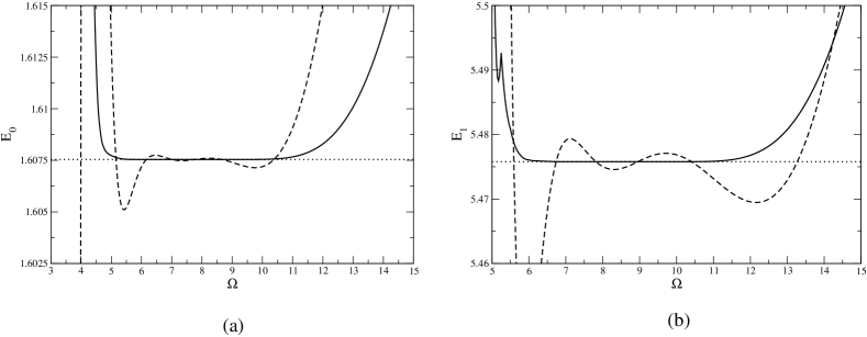
Figure 1: Comparison between the ground state (a) and first excited state (b) energy of the quartic oscillator calculated to order $15$ directly through the expansion of Eq. (5) (dashed) and the one calculated as $\langle\psi_{i}|H|\psi_{i}\rangle$, with $\psi_{i}$ at the same order ($i=0,1$), as a function of the arbitrary parameter $\Omega$. The dotted line is the result of Ref. mei97 . We use $m=1/2$, $\omega=2$ and $\mu=8$.

Figure 2: Comparison between the ground state (a) and first excited state (b) energy of the quartic oscillator calculated through the expansion of the energy (squares) and the one calculated as $\langle\psi_{i}|H|\psi_{i}\rangle$ (crosses). The dotted line is the result of Ref. mei97 . We use $m=1/2$, $\omega=2$ and $\mu=8$.

Given the perturbative nature of the approach that we are using, all the results, obtained to a finite order in perturbation theory, will display a dependence upon the arbitrary frequency $\Omega$. However this dependence is artificial since the solution of Eq. (4) does not depend upon $\Omega$. In the framework of the LDE such dependence is minimized by applying the Principle of Minimal Sensitivity (PMS) Ste81 , i.e. by requiring that a given observable $O$ (the energy, for example) be locally independent of $\Omega$:

$$\frac{\partial O}{\partial\Omega}=0.$$ (6)

In the present work we will enforce the PMS by using the energy of the state as the observable. We need however to make an important point: By solving the equations corresponding to the different perturbative orders, we obtain two different estimates of the energy of the solution. One corresponds to the expansion in Eq. (5), which was indeed used in AAD03 ; the other corresponds to calculating the energy as the expectation value of the Hamiltonian in the state described by the wave function obtained in Eq. (5). This second choice turns out to provide a much better estimate of the energy: As a matter of fact, the energy calculated in this way not only contains contributions of higher order in $\delta$ (the expectation value of the Hamiltonian is bilinear in the wave function) but it is also constrained by the variational principle (at least for the ground state) to lie above the exact result. Therefore the PMS applied to the expectation value of the Hamiltonian corresponds, for the ground state, to the statement of the variational principle.

This finding is illustrated in Fig. 2, where we compare the energy of the ground and first excited states of the quartic AHO — evaluated at order 15 — to the average value of the Hamiltonian — obtained using the wave function at the same order — as a function of $\Omega$.

In Fig. 2, on the other hand, one can see the ground and first excited state energies of the quartic AHO as a function of the perturbative order $m$, obtained after application of the PMS both to $E^{(m)}_{n}$ of Eq. (5) and to $\langle\psi_{i}^{(m)}|H|\psi_{i}^{(m)}\rangle$. The faster convergence to the correct result in the latter case is quite apparent.

It is interesting that also in the case of the excited state the approach based upon the minimization of the average value of the Hamiltonian seems to satisfy a variational principle.

III Results

Let us start by comparing the accuracy of our method with the one of Ref. Bellet:1994mf which is based on a variational improvement of the ordinary perturbation theory that gives a convergent sequence of approximations.

Figure 3: Logarithm of the error for the ground state energy of the quartic oscillator as a function of the order. The dashed line is the error of Eq. (11) of Ref. Bellet:1994mf , obtained after $47$ iterations. We use $\omega=0$ and $\mu=1$.

In Fig. 3 we display the logarithm of the percentile error for the ground state energy of the quartic oscillator as a function of the approximation order. The error is defined as

$$\Delta=100\times\left|\frac{E_{n}^{(m)}-E_{n}}{E_{n}}\right|,$$ (7)

where $E_{n}$ is the “exact” value of the energy of the $n$-th state and $E_{n}^{(m)}$ the approximate estimation to order $m$. The results using the present method (crosses) are compared to the outcome of the calculation in Ref. Bellet:1994mf , obtained after 47 iterations, for the ground state of the quartic AHO (the “exact” value of $E_{0}$ is taken from Ref. Janke:1995wt ).

We now turn to compare our results with those of Ref. mei97 , where the quartic, sextic and octic AHO have been thoroughly analyzed with a method based on the generalized Bloch equation. This method calculates iteratively certain matrix elements of the wave operator (wave function expansion coefficients) and then uses a renormalization technique.

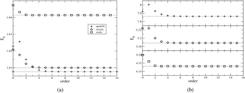
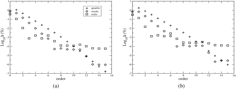
Figure 4: Energy of the ground state of the quartic, sextic and octic anharmonic oscillators, as a function of the approximation order, compared with the results of Ref. mei97 (dotted). We assume $m=1/2$ and $\omega=2$; $\mu=(8,12,16)$, respectively, in panel (a) and $\mu=(1600,2400,3200)$, respectively, in panel (b).

Figure 5: Logarithm of the error, with respect to the results of Ref. mei97 , of the energy of the ground state of the quartic, sextic and octic anharmonic oscillators, as a function of the approximation order. We assume $m=1/2$ and $\omega=2$; $\mu=(8,12,16)$, respectively, in panel (a) and $\mu=(1600,2400,3200)$, respectively, in panel (b).

In Fig. 5 we display the energy of the ground state of the quartic, sextic and octic AHO, as a function of the approximation order, compared with the results of Ref. mei97 . We have chosen the parameters of the AHO in such a way to correspond to the cases $\beta=2$ (panel (a)) and $\beta=400$ (panel (b)). Note that the values of Ref. mei97 have been obtained using 100 basis functions and several tens or hundreds of iterations.

In Fig. 5 we report, for the same cases of Fig. 5, the percentile error, defined as in Eq. (7), but taking now for $E_{n}$ the value calculated in Ref. mei97 . In other words, in Fig. 5 one can see, order by order, the discrepancy of our results from those of Ref. mei97 . It is apparent that even for relatively low orders the agreement is quite good.

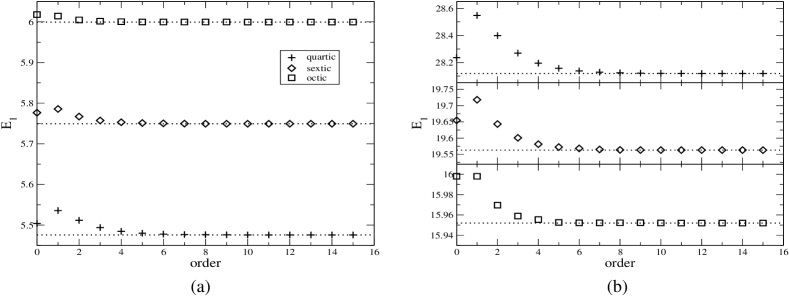
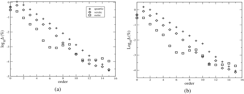
Figure 6: Energy of the first excited state of the quartic, sextic and octic anharmonic oscillators, as a function of the approximation order, compared with the results of mei97 (dotted). We assume $m=1/2$ and $\omega=2$; $\mu=(8,12,16)$, respectively, in panel (a) and $\mu=(1600,2400,3200)$, respectively, in panel (b).

Figure 7: Logarithm of the error, with respect to the results of mei97 , of the energy of the first excited state of the quartic, sextic and octic anharmonic oscillators, as a function of the approximation order. We assume $m=1/2$ and $\omega=2$; $\mu=(8,12,16)$, respectively, in panel (a) and $\mu=(1600,2400,3200)$, respectively, in panel (b).

The same considerations apply also to the excited states of the oscillators we are studying, as can be inferred from Figs. 7 and 7, which display the same quantities (energy and error) of Figs. 5 and 5, but for the first excited state.

Table 1: Energies of the ground state and of the first excited state calculated with our method to order $15$ and compared to the case $\beta=2$ in Table III of mei97 . The correct digits are underlined.

	quartic	sextic	octic
$E_{0}$	1.6075413	1.6099319	1.6413713
$E_{0}$ (Ref.mei97 )	1.607541302	1.609931952	1.6413703
$E_{1}$	5.4757859	5.7493494	5.9996138
$E_{1}$ (Ref.mei97 )	5.475784536	5.749347753	5.999607360

Table 2: As in Table 2, but for the case $\beta=400$ in Table III of mei97 . The correct digits are underlined.

	quartic	sextic	octic
$E_{0}$	7.8618628	5.188359	4.1461938
$E_{0}$ (Ref.mei97 )	7.8618627	5.1883589	4.1461886
$E_{1}$	28.118479	19.563145	15.952016
$E_{1}$ (Ref.mei97 )	28.118454	19.563130	15.951985

In Tables 2 and 2 we report the actual values of the energies of the ground state and of the first excited state calculated with our method to order $15$ and compared to the results of Ref. mei97 , with AHO parameters corresponding to the cases $\beta=2$ and $\beta=400$ of that reference, respectively.

Good accuracy is also obtained for the wave functions. In Fig. 8 one can see the ground state and the first excited state wave functions of the quartic AHO as obtained in our approximation and by direct numerical calculation.

The numerical calculation was performed using a Fortran program. We have tested the accuracy of the program by calculating the wave function of the harmonic oscillator and comparing it to the exact result. The error defined as $\Delta_{\psi}(x)=100\times\left|(\psi^{(\text{num})}(x)-\psi^{(\text{exact})}(x))/\psi^{(exact)}(x)\right|$ is found to be smaller than $10^{-7}$ in the region where the wave function is sizable. As a result, a meaningful comparison of our approximate results with the numerical results is possible.

Actually, the two curves in Fig. 8 are not distinguishable from each other at the scale of the figures: For this reason we display also the ratio of the approximate to the exact wave function.

Figure 8: Wave function for the ground state (a) and the first excited state (b) of the quartic anharmonic oscillator. The solid line is the numerical result, the dashed line (not visible) is the approximation to order $15$ of our method. The dotted line show the ratio $R(x)=\psi_{i}^{\text{(appr)}}(x)/\psi_{i}^{\text{(num)}}(x)$ of the approximate to the numerical wave function. We assume $m=1/2$, $\omega=2$ and $\mu=8$.

IV Conclusions

In Ref. AAD03 a new method for the solution of the Schrödinger equation was introduced. It is based on the application of the linear delta expansion (optimized perturbation theory) and an ansatz for the wave function that explicitly takes into account its asymptotic behavior. The new method was applied to calculate the energies and wave functions of the ground and first excited state of the quartic anharmonic potential.

In this paper we have extended the results of Ref. AAD03 in two ways, first we have computed the energies by evaluating the expectation value of the Hamiltonian at a given order using the wave function obtained with the method and shown that the accuracy obtained is greater. Secondly, we have extended the results by computing the energies and wave functions of the ground and first excited states for the quartic, sextic and octic potentials. We have verified that the method works very well for these potentials and that in fact one is able to obtain high accuracy with only a few perturbative orders. We have also presented quantitative comparisons between our results and other methods found in the literature.

- (1) Large Order Behavior of Perturbation Theory, Current Physiscs – Sources and Comments, Vol. 7, edited by J. C. Le Guillou and J. Zinn-Justin (North-Holland, Amsterdam, 1990).
- (2) T. Hatsuda, T. Kunihiro, and T. Tanaka, Phys. Rev. Lett. 78, 3229 (1997) [hep-th/9612097].
- (3) C. M. Bender and L. M. A. Bettencourt, Phys. Rev. D 54, 7710 (1996) [hep-th/9607074].
- (4) R. Guida, K. Konishi, and H. Suzuki, Ann. Phys. (N.Y.) 241, 152 (1995) [hep-th/9407027].
- (5) W. Janke and H. Kleinert, Phys. Rev. Lett. 75, 2787 (1995).
- (6) V. I. Yukalov, Phys. Rev. A 58, 96 (1998); J. Math. Phys. 32, 1235 (1991); Teor. Mat. Fiz. 28 (1976) 92.
- (7) A. Okopińska, Phys. Rev. D 35, 1835 (1987).
- (8) A. Duncan and M. Moshe M, Phys. Lett. B 215, 352 (1988).
- (9) P. M. Stevenson, Phys. Rev. D 23, 2916 (1981).
- (10) P. Amore, A. Aranda, and A. De Pace, quant-ph/0304043 (2003).
- (11) A. Pathak and S. Mandal, Phys. Lett. A 298, 259 (2002).
- (12) Y. Meurice, quant-ph/0202047 (2002).
- (13) H. Meissner and O. Steinborn, Phys. Rev. A 56, 1189 (1997).
- (14) B. Bellet, P. Garcia and A. Neveu, Int. J. Mod. Phys. A 11, 5587 (1996) [hep-th/9507155].
- (15) H. Kleinert and W. Janke W., Phys. Lett. A 206, 283 (1995) [quant-ph/9502019] .