Minimization of nonresonant effects in a scalable Ising spin quantum computer

Abstract

The errors caused by the transitions with large frequency offsets (nonresonant transitions) are calculated analytically for a scalable solid-state quantum computer based on a one-dimensional spin chain with Ising interactions between neighboring spins. Selective excitations of the spins are enabled by a uniform gradient of the external magnetic field. We calculate the probabilities of all unwanted nonresonant transitions associated with the flip of each spin with nonresonant frequency and with flips of two spins: one with resonant and one with nonresonant frequencies. It is shown that these errors oscillate with changing the gradient of the external magnetic field. Choosing the optimal values of this gradient allows us to decrease these errors by 50%.

I Introduction

Even with no interaction with the environment, errors in a quantum computer driven by radio-frequency (rf) pulses may be generated by the nonresonant action of these pulses on different spins. (See, for example, Lopez ; Method .) These errors depend on the value of the detuning from the resonant (useful) transitions. Unwanted transitions with small detunings produce the largest errors. Such transitions, called near-resonant transitions, are associated with interactions between the spins in the chain. These interactions are required in order to implement the conditional quantum logic. But the same interactions can cause unwanted transitions characterized by small detunings from resonance and relatively large probabilities. If one wants to flip the $k$th spin in a particular state and does not want to flip the same spin in the other state with different orientations of the neighboring $(k+1)$th and $(k-1)$th spins, then first of all one has to suppress these near-resonant transitions. For example, if the resonant transition is

$$|\dots 0_{k-1}0_{k}1_{k+1}\dots\rangle\rightarrow|\dots 0_{k-1}1_{k}1_{k+1}\dots\rangle,$$ (1)

then the (unwanted) near-resonant transitions to be suppressed are

$$|\dots 0_{k-1}0_{k}0_{k+1}\dots\rangle\rightarrow|\dots 0_{k-1}1_{k}0_{k+1}\dots\rangle,~{}~{}~{}|\dots 1_{k-1}0_{k}1_{k+1}\dots\rangle\rightarrow|\dots 1_{k-1}1_{k}1_{k+1}\dots\rangle.$$ (2)

A general approach for the complete suppression of near-resonant transitions for an arbitrary superposition of quantum sates in a scalable Ising spin quantum computer was developed in Method .

Since a wavelength of a rf pulse is much larger than a distance between the spins, the pulse affects all spins in the chain. Hence, in order to allow a selective excitation of the $k$th spin, one must make the Larmor frequency of this particular spin different from the Larmor frequencies of all other spins, and choose the frequency of the rf pulse to be equal to the transition frequency of this $k$th spin. In Kane’s Kane semiconductor quantum computer proposal this can be done by applying a voltage to the $k$th qubit. The approach used in this paper, is to apply a permanent magnetic field with a large gradient in the direction of the spin chain g1 ; g3 ; g2 . Because of the magnetic field gradient, the magnetic field is different for different spins, so that each spin has its unique Larmor frequency.

However, the differences in Larmor frequencies of different spins do not completely solve the problem of selective excitations. Even if these differences are large, there are small probabilities of excitations of unwanted spins with large detunings. This problem is not very important in conventional nuclear magnetic resonance spectroscopy nor for a quantum computer with a small number of qubits, since the pulse sequences do not contain a very large number of pulses. Unlike this, in a quantum computer with sufficiently large number of qubits the implementation of logic operations requires thousands of pulses. The errors caused by the nonresonant transitions, being small for a single pulse, in general grow linearly Method with the number of pulses, so that eventually accumulation of this type of error would impose severe restrictions on the number of qubits in a nuclear or electron spin quantum computer. This problem is especially acute because there are no error correction codes for correction of this type of error.

In this paper we develop an approach which allows one to decrease significantly (by 50%) the probabilities of unwanted nonresonant transitions in order to decrease the errors caused by the rf pulses of quantum protocols. Our approach to this problem is similar to the method used for minimization of errors caused by the near-resonant transitions Lopez . Since the probabilities of unwanted nonresonant transitions oscillate in time with frequencies proportional to the differences in the Larmor frequencies between the spins, one can select the optimal values of these frequency differences (by applying a specific magnetic field gradient) to minimize the nonresonant transitions. In spite of a rather refined character of our model (in the sense that this system is complicated for the experimental realization with a solid-state device), we believe that our approach provides an important tool for the solution of similar problems in many nuclear and electron spin quantum computer proposals.

II The Ising spin quantum computer

The Hamiltonian for an Ising spin chain placed in an external magnetic field can be written in the form,

$$H_{n}=-\sum_{k=0}^{L-1}\omega_{k}I_{k}^{z}-2J\sum_{k=0}^{L-2}I_{k}^{z}I_{k+1}^{z}-{\Omega_{n}\over 2}\sum_{k=0}^{L-1}\left\{I_{k}^{-}\exp\left[-i\left(\nu_{n}t+\varphi_{n}\right)\right]+h.c.\right\}=H_{0}+V_{n}(t).$$ (3)

Here $\hbar=1$; $I_{k}^{\pm}=I_{k}^{x}\pm I_{k}^{y}$; $I_{k}^{x}$, $I_{k}^{y}$, and $I_{k}^{z}$ are the components of the operator of the $k$th spin $1/2$; $\omega_{k}$ is the Larmor frequency of the $k$th spin; $J$ is the Ising interaction constant; $\Omega_{n}$ is the Rabi frequency (frequency of precession around the resonant transverse field in the rotating frame); $\nu_{n}$ and $\varphi_{n}$ are, respectively, the frequency and the phase of the $n$th pulse. The Hamiltonian (3) is written for the $n$th rectangular rf pulse. We assume that the Larmor frequency difference $\delta\omega=\omega_{k+1}-\omega_{k}$ between neighboring spins is independent of the spin’s number $k$. Below we omit the index $n$ which indicates the pulse number. The long-range dipole-dipole interaction is suppressed by choosing the angle between the chain and the external permanent magnetic field to be equal to the magic angle Lopez .

In the interaction representation, the solution of the Schrödinger equation can be written in the form

$$\Psi(t)=\sum_{n}C_{q}(t)|q\rangle\exp(-iE_{q}t),$$ (4)

where $E_{q}$ and $|q\rangle$ are, respectively, the eigenvalues and eigenfunctions of the Hamiltonian $H_{0}$. The expansion coefficients satisfy the system of linear differential equations,

$$i\dot{C}_{q}(t)=-{\Omega\over 2}\sum_{l}C_{l}(t)|l\rangle\exp[i(E_{q}-E_{l}-\sigma\nu)t-i\sigma\varphi],$$ (5)

where $\sigma=1$ if $E_{q}>E_{l}$ and $\sigma=-1$ if $E_{q}<E_{l}$. The states $|l\rangle$ and $|q\rangle$ in Eq. (5) are related by a flip of one $k^{\prime}$th spin, so that the total number of terms in the right-hand side of Eq. (5) is equal to the number of qubits, $L$.

If the condition

$$\Omega<J\ll\delta\omega$$ (6)

is satisfied, the pulse effectively affects only one $k$th spin in the chain perturbation whose frequency $\omega_{k}$ is close (near-resonant) or equal (resonant) to the frequency of the pulse, $\nu$. In this approximation, one has to keep only one term (of the $L$ terms) on the right-hand side of Eq. (5) and the system of coupled differential equations (5) splits into $2^{L}/2$ independent pairs of equations perturbation ; 1000 of the form

$$i\dot{C}_{m}(t)=-{\Omega\over 2}e^{-i\left(\Delta^{pm}t-\varphi\right)}C_{p}(t),$$ (7)

$$i\dot{C}_{p}=-{\Omega\over 2}e^{i\left(\Delta^{pm}t-\varphi\right)}C_{m}(t).$$

Here the states $|m\rangle$ and $|p\rangle$ are related by a flip of the $k$th spin, $\Delta^{pm}=E_{p}-E_{m}-\nu$, and we suppose that $E_{p}>E_{m}$.

III Nonresonant transitions

In this Section, we consider the quantum dynamics which causes the nonresonant effects. To simplify the notations, we fix the states $|p\rangle$ and $|m\rangle$, the number of the resonant spin $k$, and define

$$\delta=E_{p}-E_{m}-\nu=\Delta^{pm}.$$ (8)

The solution of Eq. (7) is

$$C_{m}(t_{0}+\tau)=\left[\cos\left({\lambda\tau\over 2}\right)+i{\delta\over\lambda}\sin\left({\lambda\tau\over 2}\right)\right]e^{-i{\delta\over 2}\tau},$$ (9)

$$C_{p}(t_{0}+\tau)=i{\Omega\over\lambda}\sin\left({\lambda\tau\over 2}\right)e^{i\delta t_{0}-i\varphi+i{\delta\over 2}\tau}.$$

Here $t_{0}$ is the time of the beginning of the pulse; $\lambda=\sqrt{\delta^{2}+\Omega^{2}}$; $\tau=t-t_{0}$ is the duration of the pulse; and the initial conditions are

$$C_{m}(t_{0})=1,\qquad C_{p}(t_{0})=0.$$ (10)

The solution for the transition from the upper state to the lower state is

$$C_{m}(t_{0}+\tau)=i{\Omega\over\lambda}\sin\left({\lambda\tau\over 2}\right)e^{-i\delta t_{0}+i\varphi-i{\delta\over 2}\tau},$$

$$C_{p}(t_{0}+\tau)=\left[\cos\left(\lambda\tau\over 2\right)-i{\delta\over\lambda}\sin\left({\lambda\tau\over 2}\right)\right]e^{i{\delta\over 2}\tau},$$ (11)

$$C_{m}(t_{0})=0,\qquad C_{p}(t_{0})=1.$$

Suppose that initially only one state is populated, for example,

$$C_{m}(t_{0})=1,~{}~{}C_{p}(t_{0})=0,~{}~{}|m\rangle=|0_{4}0_{3}{\bf 0}_{2}1_{1}0_{0}\rangle,~{}~{}|p\rangle=|0_{4}0_{3}{\bf 1}_{2}1_{1}0_{0}\rangle~{}~{}(k=2).$$ (12)

The dynamics of the coefficients $C_{m}(t)$ and $C_{p}(t)$ is defined by Eq. (9). Now we calculate the probabilities for transitions associated with the flip of a spin with nonresonant frequency, and with flips of two spins: one with resonant and one with nonresonant frequencies. We consider, for example, the transitions $|m\rangle\rightarrow|i\rangle$ and $|m\rangle\rightarrow|j\rangle$, where

$$|i\rangle=|0_{4}1_{3}{\bf 0}_{2}1_{1}0_{0}\rangle,~{}~{}|j\rangle=|0_{4}1_{3}{\bf 1}_{2}1_{1}0_{0}\rangle.$$ (13)

Here $k^{\prime}=3$ is the number of the spin with the nonresonant frequency, and the initial conditions are

$$C_{i}(t_{0})=0,~{}~{}C_{j}(t_{0})=0.$$ (14)

The dynamics of these coefficients is defined by Eqs. (5) with two essential terms on the right-hand side,

$$i\dot{C}_{i}(t)=-\frac{\Omega}{2}e^{-i(\Delta t-\varphi)}C_{j}(t)-\frac{\Omega}{2}e^{i[(E_{i}-E_{m}-\sigma\nu)t-\sigma\varphi)]}C_{m}(t),$$

$$i\dot{C}_{j}(t)=-\frac{\Omega}{2}e^{i(\Delta t-\varphi)}C_{i}(t)-\frac{\Omega}{2}e^{i[(E_{j}-E_{p}-\sigma\nu)t-\sigma\varphi)]}C_{p}(t),$$ (15)

where

$$\Delta\equiv E_{j}-E_{i}-\nu;$$ (16)

$E_{j}>E_{i}$; $\sigma=1$ if $E_{i}>E_{m}$ (and $E_{j}>E_{n}$) and $\sigma=-1$ if $E_{i}<E_{m}$ (and $E_{j}<E_{n}$). For example, for the states in Eqs. (12) and (13) one has $E_{i}>E_{m}$ and $\sigma=1$. We characterize the nonresonant transition with (large) detuning $D$ (which in general depends on the kind of state and spin number $k^{\prime}$) defined as

$$D=E_{i}-E_{m}-\sigma\nu-{\delta-\Delta\over 2}.$$ (17)

Then using Eqs. (8), (16), and (17) one can write

$$E_{i}-E_{m}-\sigma\nu=D+{\delta-\Delta\over 2},~{}~{}~{}E_{j}-E_{p}-\sigma\nu=D-{\delta-\Delta\over 2}.$$ (18)

It is convenient to introduce new coefficients

$$C_{i}(t)=e^{-i\frac{\Delta}{2}t}A_{i},~{}~{}~{}C_{j}(t)=e^{i\frac{\Delta}{2}t-i\varphi}A_{j}.$$ (19)

Then one obtains a system of two coupled differential equations for the coefficients $A_{i}(t)$ and $A_{j}(t)$ with an effective oscillating external force,

$$i\dot{A}_{i}(t)+\frac{\Delta}{2}A_{i}(t)+\frac{\Omega}{2}A_{j}(t)=-\frac{\Omega}{2}e^{i\left[\left(D+\frac{\delta}{2}\right)t-\sigma\varphi\right]}C_{m}(t),$$

$$i\dot{A}_{j}(t)-\frac{\Delta}{2}A_{j}(t)+\frac{\Omega}{2}A_{i}(t)=-\frac{\Omega}{2}e^{i\left[\left(D-\frac{\delta}{2}\right)t-(\sigma-1)\varphi\right]}C_{p}(t),$$ (20)

$$A_{i}(t_{0})=0,~{}~{}~{}~{}A_{j}(t_{0})=0,$$

where $C_{m}(t)$ and $C_{p}(t)$ are defined by Eq. (9). In order to remove the constant phases from Eq. (20) we write

$$A_{i}(t)=e^{i\left[\left(D+\frac{\delta}{2}\right)t_{0}-\sigma\varphi\right]}B_{i}(\tau),~{}~{}~{}A_{j}(t)=e^{i\left[\left(D+\frac{\delta}{2}\right)t_{0}-\sigma\varphi\right]}B_{j}(\tau).$$ (21)

The coefficients $B_{i}(\tau)$ and $B_{j}(\tau)$ satisfy the following system of two coupled differential equations:

$$i\dot{B}_{i}(\tau)+\frac{\Delta}{2}B_{i}(\tau)+\frac{\Omega}{2}B_{j}(\tau)=f(\tau),$$

$$i\dot{B}_{j}(\tau)-\frac{\Delta}{2}B_{j}(\tau)+\frac{\Omega}{2}B_{i}(\tau)=g(\tau),$$ (22)

$$B_{i}(0)=0,~{}~{}~{}~{}B_{j}(0)=0,$$

where the differentiation is performed with respect to time-interval, $\tau$, and

$$f(\tau)=-\frac{\Omega}{4}\left(1+\frac{\lambda}{\delta}\right)e^{i\left(D+\frac{\lambda}{2}\right)\tau}-\frac{\Omega}{4}\left(1-\frac{\lambda}{\delta}\right)e^{i\left(D-\frac{\lambda}{2}\right)\tau},$$

$$g(\tau)=-\frac{\Omega^{2}}{4\lambda}\left[e^{i\left(D+\frac{\lambda}{2}\right)\tau}-e^{i\left(D-\frac{\lambda}{2}\right)\tau}\right].$$ (23)

By differentiation of the system of equations (22), one obtains two uncoupled second order differential equations,

$$\ddot{B}_{i}(\tau)+\frac{\Lambda^{2}}{4}B_{i}(\tau)=\frac{\Delta}{2}f(\tau)+\frac{\Omega}{2}g(\tau)-i\dot{f}(\tau),$$

$$B_{i}(0)=0,~{}~{}~{}~{}\dot{B}_{i}(0)=i\frac{\Omega}{2}$$ (24)

and

$$\ddot{B}_{j}(\tau)+\frac{\Lambda^{2}}{4}B_{j}(\tau)=-\frac{\Delta}{2}g(\tau)+\frac{\Omega}{2}f(\tau)-i\dot{g}(\tau),$$

$$B_{j}(0)=0,~{}~{}~{}~{}\dot{B}_{j}(0)=0,$$ (25)

where the initial conditions for $\dot{B}_{i}(0)$ and $\dot{B}_{j}(0)$ follow from Eq. (22) with $f(0)=-\Omega/2$ and $g(0)=0$.

The solution for both coefficients $B_{i}(\tau)$ and $B_{j}(\tau)$ has the form,

$$a_{1}e^{i\frac{\Lambda}{2}\tau}+a_{2}e^{i\frac{\Lambda}{2}\tau}+a_{3}e^{i\left(D+\frac{\lambda}{2}\right)\tau}+a_{4}e^{i\left(D-\frac{\lambda}{2}\right)\tau}$$

with different coefficients $a_{1},\dots,a_{4}$. Keeping only first order terms in $\Omega/D$, one obtains,

$$B_{i}(\tau)=-{\Omega\over 2D}\left\{\cos\left({\Lambda\tau\over 2}\right)-\left[\cos\left({\lambda\tau\over 2}\right)+i\frac{\delta}{\lambda}\sin\left({\lambda\tau\over 2}\right)\right]e^{iD\tau}\right\},$$

$$B_{j}(\tau)=-i{\Omega\over 2D}\left\{\frac{\Omega}{\Lambda}\sin\left({\Lambda\tau\over 2}\right)-\frac{\Omega}{\lambda}\sin\left({\lambda\tau\over 2}\right)e^{iD\tau}\right\}.$$ (26)

This solution is written for the initial condition (10). For the initial conditions given by the third equation (11), the solution is

$$B_{i}^{\prime}(\tau)=-i{\Omega\over 2D}\left\{\frac{\Omega}{\Lambda}\sin\left({\Lambda\tau\over 2}\right)-\frac{\Omega}{\lambda}\sin\left({\lambda\tau\over 2}\right)e^{iD\tau}\right\},$$

$$B_{j}^{\prime}(\tau)=-{\Omega\over 2D}\left\{\cos\left({\Lambda\tau\over 2}\right)-\left[\cos\left({\lambda\tau\over 2}\right)-i\frac{\delta}{\lambda}\sin\left({\lambda\tau\over 2}\right)\right]e^{iD\tau}\right\}.$$ (27)

Here the coefficients $B_{i}^{\prime}(\tau)$ and $B_{j}^{\prime}(\tau)$ are obtained using Eq. (11) and the properly modified relations (19) and (21) (which result in different common phase factors, unimportant for further consideration).

IV Probabilities of nonresonant transitions

The nonresonant transitions considered in the previous Section generate errors in the quantum computer. Our objective is to minimize the probabilities of these transitions (for estimations of these probabilities see Refs. perturbation ; 1000 ; Felix1 ) as much as possible by choosing optimal parameters of the model. As follows from Eq. (26), the probability of a nonresonant transitions associated with the flip of a spin with nonresonant frequency is proportional to $(\Omega/2\delta\omega)^{2}$. (See also Refs. perturbation ; 1000 .) If one could suppress these transitions, the total probability of error would be associated with flips of two spins with nonresonant frequencies, and it would be of order of $(\Omega/2\delta\omega)^{4}$. Successful solution of this problem would allow one to substantially decrease the errors introduced by the rf pulses and to relieve the requirements for large magnetic field gradients characterized by $\delta\omega$.

In order to estimate the errors given by Eq. (26), we will analyze this equation for a typical example. Consider the errors generated during implementation of the (useful) transition

$$|m\rangle\rightarrow|p\rangle,$$ (28)

where the states $|m\rangle$ and $|p\rangle$ are defined in Eq. (12). Since the frequency of the external rf field is resonant for this transition, then

$$\nu=E_{p}-E_{m}=3\delta\omega,~{}~{}~{}\delta=0~{}~{}~{}\lambda=\Omega,~{}~{}~{}\tau={\pi\over\Omega}~{}~{}~{}k=2,$$ (29)

where $k$ is the number of the spin with the resonant frequency.

The values

$$\Delta_{k^{\prime}},~{}~{}~{}~{}\lambda_{k^{\prime}}=\sqrt{\Delta^{2}_{k^{\prime}}+\Omega^{2}}$$ (30)

for nonresonant transitions to the states with one flipped $k^{\prime}$ spin are

$$\Delta_{k^{\prime}}=\delta,~{}~{}~{}\Lambda_{k^{\prime}}=\lambda~{}~{}~{}{\rm if}~{}~{}~{}k^{\prime}\neq k\pm 1.$$ (31)

When $k^{\prime}=\pm 1$ the detunings are different, $\Delta_{k^{\prime}}\neq\delta$, and depend on the orientations of the $(k+1)$th and $(k-1)$th spins in the state $|i\rangle$. For example, for the states in Eq. (13) one has $E_{j}-E_{i}=3\delta\omega-2J$ so that

$$\Delta_{3}=E_{j}-E_{i}-\nu=\delta-2J=-2J.$$ (32)

For the detunings associated with the other spins, one has

$$\Delta_{0}=0,~{}~{}~{}\Delta_{1}=2J~{}~{}~{}\Delta_{4}=0.$$ (33)

In order to produce resonant transitions (where $\delta=0$), the time-interval should be $\tau=\pi/\Omega$ [$\pi$-pulse, see Eq. (9)]. In order to suppress possible near-resonant transitions, the value of $\Omega$ should satisfy the $2\pi K$-condition Lopez

$$\Omega^{(K)}={2J\over\sqrt{4K^{2}-1}}.$$ (34)

For these parameters and for the state $|m\rangle$ in Eq. (12) (for $k=2$) the quantities in Eq. (26) take the following values:

$$\delta=0,~{}~{}~{}\lambda=\Omega,~{}~{}~{}\sin\left({\lambda\tau\over 2}\right)=1,~{}~{}~{}\cos\left({\lambda\tau\over 2}\right)=0,$$

$$\sin\left({\Lambda_{k^{\prime}}\tau\over 2}\right)=1,~{}~{}~{}\cos\left({\Lambda_{k^{\prime}}\tau\over 2}\right)=0,~{}~{}~{}{\rm for}~{}~{}~{}{k^{\prime}\neq k\pm 1},$$ (35)

$$\sin\left({\Lambda_{k^{\prime}}\tau\over 2}\right)=0,~{}~{}~{}\cos\left({\Lambda_{k^{\prime}}\tau\over 2}\right)=1,~{}~{}~{}{\rm for}~{}~{}~{}{k^{\prime}=k\pm 1}.$$

Then, after the $\pi$-pulse the coefficients in Eq. (26) become

$$B_{i}^{k^{\prime}}=0,~{}~{}~{}B_{j}^{k^{\prime}}=-i{\Omega\over 2D_{k^{\prime}}}\left(1-e^{i\pi{D_{k^{\prime}}\over\Omega}}\right)~{}~{}~{}{\rm for}~{}~{}~{}k^{\prime}\neq k\pm 1,$$ (36)

and

$$B_{i}^{k^{\prime}}=-{\Omega\over 2D_{k^{\prime}}},~{}~{}~{}B_{j}^{k^{\prime}}=i{\Omega\over 2D_{k^{\prime}}}e^{i\pi{D_{k^{\prime}}\over\Omega}}~{}~{}~{}{\rm for}~{}~{}~{}k^{\prime}=k\pm 1,$$ (37)

where the upper index of the amplitudes $B_{i}^{k^{\prime}}$ and $B_{j}^{k^{\prime}}$ indicates that these states are associated with the initial state by the flip of the $k^{\prime}$th spin.

The coefficients $B_{i}^{k^{\prime}}$ and $B_{j}^{k^{\prime}}$ in Eqs. (36) and (37) are calculated for a transition resonant for the initial state. If the frequency of the rf pulse is close to resonant (near-resonant), then

$$\delta\neq 0,~{}~{}~{}\lambda=\sqrt{\Omega^{2}+4J^{2}},~{}~{}~{}\sin\left({\lambda\tau\over 2}\right)=0,~{}~{}~{}\cos\left({\lambda\tau\over 2}\right)=1,$$

$$\sin\left({\Lambda_{k^{\prime}}\tau\over 2}\right)=0,~{}~{}~{}\cos\left({\Lambda_{k^{\prime}}\tau\over 2}\right)=1,~{}~{}~{}{\rm for}~{}~{}~{}{k^{\prime}\neq k\pm 1},$$ (38)

$$\sin\left({\Lambda_{k^{\prime}}\tau\over 2}\right)=1,~{}~{}~{}\cos\left({\Lambda_{k^{\prime}}\tau\over 2}\right)=0,~{}~{}~{}{\rm for}~{}~{}~{}{k^{\prime}=k\pm 1}.$$

Figure 1: Probability of errors after application of $\pi$-pulse resonant for the transition (28) for states and initial conditions defined in Eq. (12). The solid line indicates the analytic results calculated using Eq. (39).The filled circles are calculated using exact numerical solution perturbation ; 1000 . $L=5$, $\Omega/J=\Omega^{(K)}/J\approx 1/2$, $K=2$ [see Eq. (34)].

The error $P_{k}$ for an arbitrary initial state generated by the pulse resonant for the transition (1) is the sum of the probabilities of all nonresonant transitions associated with flips of all spins with $k^{\prime}\neq k$,

$$P_{k}=2\left({\Omega\over 2D_{k-1}}\right)^{2}+2\left({\Omega\over 2D_{k+1}}\right)^{2}+\sum_{k^{\prime}\neq k-1,k,k+1}\left({\Omega\over 2D_{k^{\prime}}}\right)^{2}\left|1-e^{i\pi{D_{k^{\prime}}\over\Omega}}\right|^{2}.$$ (39)

If $k=1$ then the term with $D_{k-1}$ in Eq. (39) should be omitted. If $k=L-1$, one must omit the term with $D_{k+1}$. In Fig. 1 we plot the total probability of error after application of a $\pi$-pulse resonant for the transition (28) with the states and initial conditions defined in Eq. (12). One can see a good correspondence between the numerical and analytical results. The same agreement was observed for other initial states and parameters of the model. The parameters used in the simulations can be realized using, for example, phosphorus impurity donors in silicon. (For the relation between the numerical and physical parameters, see, for example, Ref. Method .)

V Minimization of nonresonant transitions

From Eq. (39) and Fig. 1 one can see that probability of error oscillates as a function of the ratio $\delta\omega/\Omega$. As follows from Eq. (39) the period of oscillations is equal to 2. (In Fig. 1 the period is twice smaller because of the symmetry of the transition: the probabilities oscillate only for the transitions with detunings of the order of $2\delta\omega$.)

In order to describe these oscillations we continue to analyze the example from the previous Section. The values of $D_{k^{\prime}}$ for the initial state $|m\rangle$ in Eq. (12) and for $k=2$ are

$$D_{0}=-2\delta\omega-J,~{}~{}D_{1}=\delta\omega-J,~{}~{}D_{4}=\delta\omega+J,~{}~{}D_{5}=2\delta\omega+J.$$ (40)

Under the condition

$$|{D_{0}\over\Omega}|=|{D_{5}\over\Omega}|=2q,$$ (41)

all (two) terms in the sum in Eq. (39) vanish, and the probability of error takes its minimum value equal to

$$P^{\rm min}\approx\left({\Omega\over\delta\omega}\right)^{2}\approx{1\over q^{2}}.$$ (42)

For example, in Fig. 2 for $\delta\omega/\Omega\approx q=194$ one has $P^{\rm min}\approx 2.65\times 10^{-5}$.

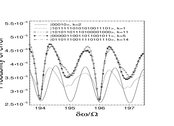
Figure 2: The same as Fig. 1 but for different states. The results are obtained using Eq. (39).

We analyzed the nonresonant transitions only for one state. We now discuss the general case. In Fig. 2 we plot the probabilities of errors for four randomly selected states generated by the pulse, resonant for the transition (1) for $L=20$ qubits. For comparison, we also plot the curve from Fig. 1 (solid line) analyzed before. In principle, one could calculate errors for an arbitrary number of qubits. However, since the probabilities of flips of distant qubits decrease as $1/(k-k^{\prime})^{2}$, the distant qubits do not contribute significantly to the total error.

From Fig. 2 one can see that errors for different states take their minimum values at the same values of $\delta\omega/\Omega$. It is convenient to write the detunings $D_{kk^{\prime}}$ (here $k$ is the number of spin with the resonant or near-resonant frequency, and $k^{\prime}$ is the number of spin with nonresonant frequency) in the form

$$|D_{kk^{\prime}}|=|k-k^{\prime}|\delta\omega+\alpha_{kk^{\prime}}J,$$ (43)

where $\alpha_{kk^{\prime}}$ can assume the integer values $-2,-1,0,1,2$. Choosing the parameters

$${\delta\omega\over\Omega}=2Q,~{}~{}~{}K=2{\cal K},$$ (44)

where $Q\gg 1$ and ${\cal K}$ are integers, one can write

$$\left|{D_{kk^{\prime}}\over\Omega}\right|\approx 2Q|k-k^{\prime}|+\alpha_{kk^{\prime}}\left(2{\cal K}-{1\over 16{\cal K}}\right).$$ (45)

Here we used Eq. (34). The value of $Q\gg 1$ defines the magnetic field gradient characterized by the ratio $\delta\omega/\Omega$, and ${\cal K}\geq 1$ determines the Rabi frequency, or $\Omega/J$ at a given value of the Ising interaction constant $J$.

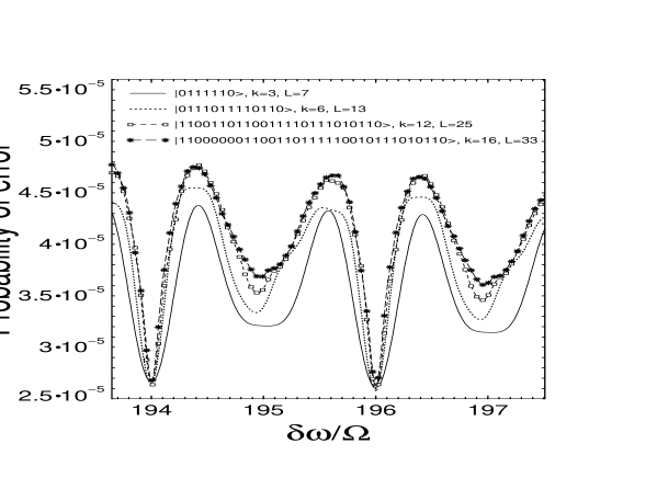
Figure 3: The error for different number $L$ of spins in the spin chain. k is chosen in the center of the chain when the error takes its maximum value. ${\cal K}=1$.

Under the conditions (44) the errors $P_{kk^{\prime}}$ associated with flips of $k^{\prime}$th spins with $k^{\prime}\neq k,k\pm 1$ (below called the distant spins) in the sum of Eq. (39) take their minimum values equal to

$$P_{kk^{\prime}}\approx{1\over 4Q^{2}}\left({\pi\over 32{\cal K}}\right)^{2}\left({\alpha_{kk^{\prime}}\over k-k^{\prime}}\right)^{2}.$$ (46)

At the minimums, the transitions associated with the flips of the distant spins are mostly suppressed, and the total error (42) is mainly associated with flips of the $(k-1)$th and the $(k+1)$th spins,

$$P_{k}^{\rm min}\approx{1\over 4Q^{2}}\left[1-{2{\cal K}\over Q}(\alpha_{k,k-1}+\alpha_{k,k+1})\left(1-{1\over 32{\cal K}^{2}}\right)+\left({\pi\over 32{\cal K}}\right)^{2}\sum_{k^{\prime}\neq k-1,k,k+1}\left({\alpha_{kk^{\prime}}\over k-k^{\prime}}\right)^{2}\right].$$ (47)

From this equation one can see that even for minimum value ${\cal K}=1$, the error associated with flips of distant spins is at least two orders smaller than the error associated with flips of $(k+1)$th and $(k-1)$th spins, and this error quickly decreases as ${\cal K}$ increases.

Since the transitions associated with flips of the distant spins are mostly suppressed, for the optimal parameters (44) the error is practically independent of the number of qubits. In Fig. 3 we compare the errors generated by nonresonant transitions for different numbers of spins in the spin chain. From Fig. 3 one can see that, in general, the error grows as the number of qubits increases, but the error in the minima is almost independent of the number of qubits $L$.

Figure 4: Probabilities of unwanted states created in result of the $\pi$-pulse resonant to the transition (1). Initial state is $|11010111001\rangle$, $k=5$, $L=11$, ${\cal K}=5$ ($\Omega/J\approx 0.1$); (a) $\delta\omega/\Omega=200$ ($Q=100$), (b) $\delta\omega/\Omega=200.314$. The results are obtained using exact numerical solution perturbation ; 1000 .

It is important that the error is associated only with the $(k+1)$th, $k$th, and the $(k-1)$th spins. The probabilities of flips of other spins are small when the condition (44) is satisfied. In Figs. 4(a,b) the probabilities of error are plotted for different states for the optimal value $\delta\omega/\Omega=2Q=200$ [Fig. 4(a)], and for another value $\delta\omega/\Omega=200.314$ [Fig. 4(b)]. By comparison of Fig. 4(a) and Fig. 4(b), one can see that optimization of the parameters results in the relative suppression of all but four transitions, associated with flips of $(k-1)$th, $k$th, and $(k+1)$th spins. Since the errors are associated with the definite three spins these errors, probably, can be corrected by application of error-correction codes associated with these particular spins.

VI Conclusion

In this paper, we considered the effect of suppression of nonresonant transitions only for one pulse. Since a quantum protocol consists of many such pulses, application of our results would substantially decrease the rate with which the error accumulates in the register of a quantum computer.

In our model the Larmor frequency $w_{0}+k^{\prime}\delta\omega$ of the $k^{\prime}$th spin increases with increasing spin number $k^{\prime}$. If $k$ is the number of the spin with resonant frequency, then the moduli of detunings $\delta\omega|k-k^{\prime}|$ increase with increasing “distance” $|k-k^{\prime}|$, so that the error associated with flips of distant spins decreases as $1/(k-k^{\prime})^{2}$. The situation is different for Kane’s quantum computer Kane . In this computer the Larmor frequencies are the same for different spins, except for one spin whose frequency is changed by application of a voltage to this particular spin. Hence, the detunings are the same for all spins in the chain (except for the one spin to which the voltage is applied) and equal to $\delta\omega$. As a result, the error caused by the nonresonant transitions should increase linearly with an increase in the number of qubits. Our method would allow one to suppress this linear growth.

References

• (1) G. P. Berman, G. D. Doolen, G. V. LΓ²pez, and V. I. Tsifrinovich, Phys. Rev. A 61, 062305 (2000).
• (2) G. P. Berman, D. I. Kamenev, R. B. Kassman, C. Pineda, and V. I. Tsifrinovich, Int. J. Quant. Inf. 1, 51 (2003); quant-ph/0212070.
• (3) B. E. Kane, Nature (London) 393, 133 (1998).
• (4) M. DrndiΔ‡, K. S. Johnson, J. H. Thywissen, M. Prentiss, and R. M. Westervelt, Appl. Phys. Lett. 72, 2906 (1998).
• (5) J. R. Goldman, T. D. Ladd, F. Yamaguchi, and Y. Yamamoto, Appl. Phys. A 71, 11 (2000).
• (6) D. Suter and K. Lim, Phys. Rev. A 65, 052309 (2002).
• (7) G. P. Berman, G. D. Doolen, D. I. Kamenev, and V. I. Tsifrinovich, Phys. Rev. A 65, 012321 (2002).
• (8) G.P. Berman, D.I. Kamenev, and V.I. Tsifrinovich, J. Appl. Math. 3, 35 (2003); quant-ph/0110069.
• (9) G. P. Berman, F. Borgonovi, G. Celardo, F. M. Izrailev, and D. I. Kamenev, Phys. Rev. E 66, 056206 (2002).