Fast light, slow light, and phase singularities: a connection to generalized weak values

Abstract

We demonstrate that Aharonov-Albert-Vaidman (AAV) weak values have a direct relationship with the response function of a system, and have a much wider range of applicability in both the classical and quantum domains than previously thought. Using this idea, we have built an optical system, based on a birefringent photonic crystal, with an infinite number of weak values. In this system, the propagation speed of a polarized light pulse displays both superluminal and slow light behavior with a sharp transition between the two regimes. We show that this system’s response possesses two-dimensional, vortex-antivortex phase singularities. Important consequences for optical signal processing are discussed.

The role of measurement in quantum mechanics has posed challenges for physicists for nearly a century. Standard quantum mechanics represents ideal measurements as the action of a Hilbert-space operator on a state. In an ideal or “strong” measurement, the operator completely collapses the state into an eigenstate, with an expectation value within the range of the operator’s eigenvalues. Strong measurements yield maximal information about the state of the system and correspond to most laboratory measurements.

Contrary to traditional quantum measurement theory, certain experiments can return results that are far beyond the range of an observable’s eigenvalues Aharonov1988 . These so-called “weak” measurements barely perturb the state, and have been less studied in quantum mechanics because they yield very little information. In their seminal work, Aharonov, Albert and Vaidman (AAV) showed that paradoxical results can be obtained if one preselects an initial state, performs a weak measurement, and subsequently a standard strong measurement which postselects a particular final state. Although the action of the weak measurement has little effect on the global state of the system, it can have a significant impact on one or more of its components. Weak values have been theoretically discussed for spin-$1/2$ particles and experimentally demonstrated in optical systems involving the angular deflections of polarized light beams passing through birefringent prisms Aharonov1988 ; Duck1989 ; Knight1990 ; Ritchie1991 .

Recently, using the approach of quantum-trajectory theory, it has been demonstrated that postselected weak values can be thought of as quantum correlation functions, which can be used in quantum optics and related areas Wiseman2002 . In this paper, we instead start from the original derivation of the AAV effect and extend it further.

We show that weak values appear in a natural way in a much broader range of situations. We demonstrate that a system’s response function (or scattering matrix) has a direct relationship with AAV weak values. As an illustration, we present an experimental study of a frequency-dependent, polarization-sensitive, optical system based on a two-dimensional (2D), birefringent photonic crystal. The response of this system can be described by an infinite number of unbounded weak values which physically correspond to measurements of the polarization value or spin of the photon along different axes. Unlike previously studied weak measurements, this system maps polarization states onto collinear spatial position along the direction of propagation, resulting in unbounded values for the time-of-flight of a polarized optical pulse. The system displays both superluminal Steinberg1993 ; Wang2000 and slow light Hau1999  behavior with a sharp transition between the two regimes and gives us total control over the speed of light. It may lead to several important applications in optical signal processing Lukin2001 , such as optical delay lines with polarization-tuned characteristics and dynamical optical clock multipliers. This new approach to quantum weak values should also open the door for many new precision measurements of very tiny quantities Aharonov1988 ; Duck1989 .

The complex response of a linear system parametrized by two general variables $\left(\rho,\eta\right)$ is given by

$$\tilde{T}\left(\rho,\eta\right)=\left\langle\psi_{f}\right|U\left(\rho,\eta\right)\left|\psi_{in}\right\rangle$$ (1)

where $U\left(\rho,\eta\right)$ is a unitary operator describing the evolution of the system, and $\left|\psi_{in}\right\rangle$ and $\left|\psi_{f}\right\rangle$ are normalized input and output states. To apply the AAV formalism, we must express Eq. 1 in terms of the preselection of an initial state, a weak measurement, and a strong measurement or projection onto a particular final state. The difficulty lies in the fact that $U\left(\rho,\eta\right)$ cannot be generally classified as a weak operator because it may have a strong impact on $\left|\psi_{in}\right\rangle$. However, we are free to decompose $U\left(\rho,\eta\right)$ into a large or “strong” part and a small or “weak” part. To do so, we Taylor expand the general operator $U\left(\rho,\eta\right)$ around an arbitrary point $\left(\rho_{0},\eta_{0}\right)$ for small deviations $\delta\rho$ and $\delta\eta$, and separate $U\left(\rho,\eta\right)$ into a weak operator $U_{\mathrm{W}}\left(\delta\rho,\delta\eta;\rho_{0},\eta_{0}\right)$ and a strong operator $U_{\mathrm{S}}\equiv U\left(\rho_{0},\eta_{0}\right)$ obtaining

$$\tilde{T}\left(\rho_{0}+\delta\rho,\eta_{0}+\delta\eta\right)\approx$$

$$\left\langle\psi_{f}\right.\left|\tilde{\psi}_{in}\left(\rho_{0},\eta_{0}\right)\right\rangle\left\{1+i\left[A_{\rho}\right]_{W}\delta\rho+i\left[A_{\eta}\right]_{W}\delta\eta\right\}$$ (2)

where $\left|\tilde{\psi}_{in}\left(\rho_{0},\eta_{0}\right)\right\rangle\equiv U_{\mathrm{S}}\left|\psi_{in}\right\rangle$, and $\left[A_{\rho}\right]_{W}$ and $\left[A_{\eta}\right]_{W}$ are given by:

$$\left[A_{j}\left(\rho_{0},\eta_{0}\right)\right]_{W}=\frac{\left\langle\psi_{f}\right|A_{j}\left(\rho_{0},\eta_{0}\right)\left|\tilde{\psi}_{in}\left(\rho_{0},\eta_{0}\right)\right\rangle}{\left\langle\psi_{f}\right.\left|\tilde{\psi}_{in}\left(\rho_{0},\eta_{0}\right)\right\rangle}$$ (3)

with $A_{j}\left(\rho_{0},\eta_{0}\right)=-i\left[\partial_{j}U_{\mathrm{S}}\right]U_{\mathrm{S}}^{\dagger}$ for $j\rightarrow\rho,\eta$.

The strong operator $U_{\mathrm{S}}$ can be viewed as a preselector which generates the state $\left|\tilde{\psi}_{in}\left(\rho_{0},\eta_{0}\right)\right\rangle$ from $\left|\psi_{in}\right\rangle$, and $U_{\mathrm{W}}\left(\delta\rho,\delta\eta;\rho_{0},\eta_{0}\right)$ is a weak measurement operator which acts on this preselected state. Eq. 3 then implies that $\left[A_{\rho}\right]_{W}$ and $\left[A_{\eta}\right]_{W}$ are AAV weak values associated with the operators $A_{\rho}\left(\rho_{0},\eta_{0}\right)$ and $A_{\eta}\left(\rho_{0},\eta_{0}\right)$. These weak values $\left[A_{\rho}\right]_{W}$ and $\left[A_{\eta}\right]_{W}$ can be unbounded if the corresponding transfer function has a singularity, i.e., a point for which $\left\langle\psi_{f}\right.\left|\tilde{\psi}_{in}\left(\rho_{0},\eta_{0}\right)\right\rangle=0$.

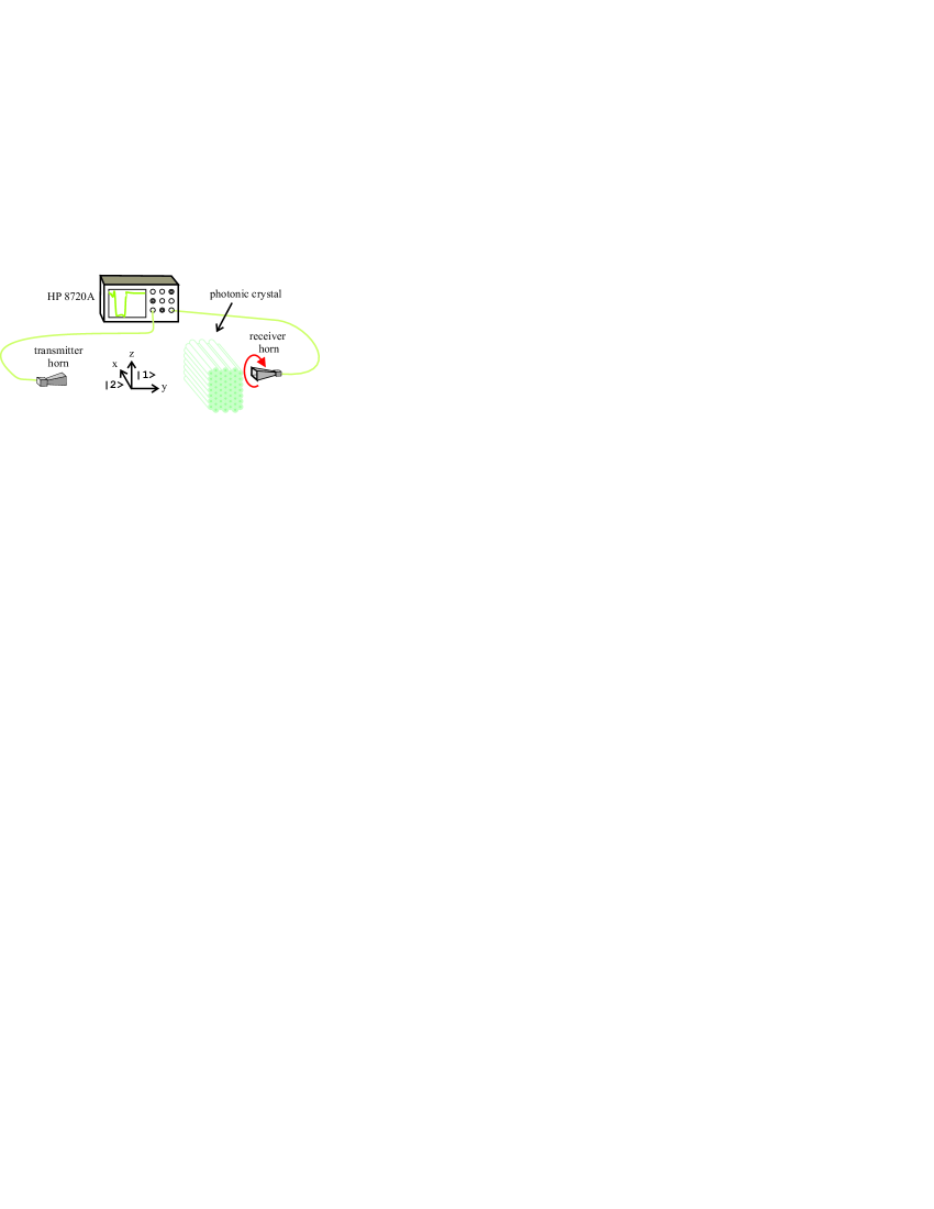
Figure 1: Experimental setup for transmission measurements.

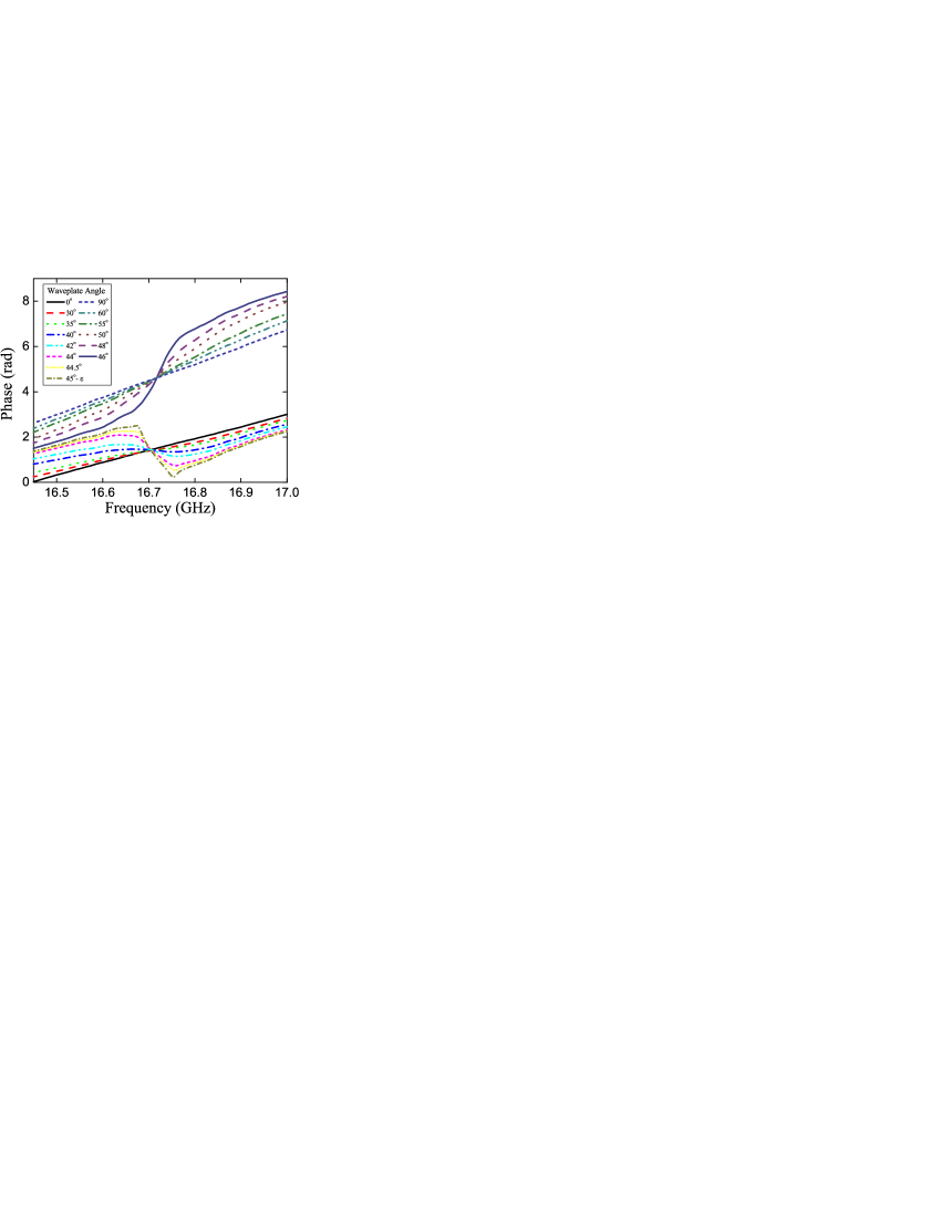
Figure 2: Experimentally measured phase delay vs. frequency for microwaves transmitted through an 18-layer photonic crystal positioned at different angles.

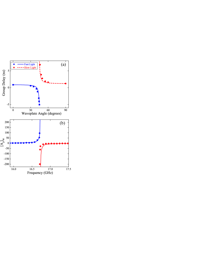
Figure 3: Experimentally measured group delay vs. crystal rotation at $\omega$ = 16.7 GHz (a) and pointer for $\left[A_{\beta}\right]_{W}$ vs. frequency at $\beta=\pi/4$ (b).

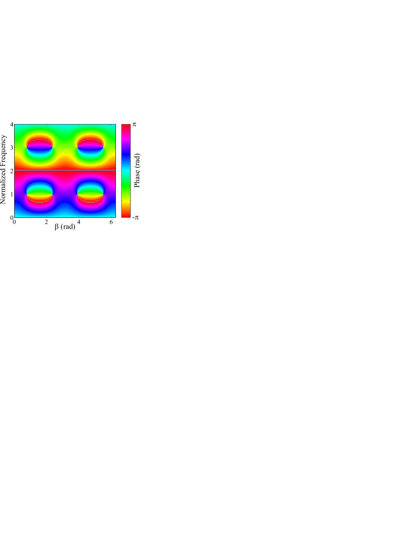
Figure 4: Theoretical contour plot of $\left[\arg\tilde{T}(\omega,\beta)\right]$ showing the singularities and the surrounding phase. The arcs connecting the singularities correspond to $2\pi$ phase slips.

This analysis is valid for classical and quantum-mechanical systems. In the quantum mechanical case, we must reinterpret $\delta\rho$ and $\delta\eta$ as operators rather than deviation parameters, while, the preselected state is a superposition of eigenstates, sharply peaked about $\rho_{0}$ and $\eta_{0}$ such that the expectation values of $\delta\rho$ and $\delta\eta$, appearing in Eq. 2, are small relative to $\rho_{0}$ and $\eta_{0}$, respectively.

Experimentally observable quantities are inferred from an indicator or pointer on a measuring device. In the general case, $\delta\rho$ and $\delta\eta$ are canonical variables describing two independent measuring devices. The pointers of these measuring devices are the conjugate momenta to these canonical variables, and the interaction weak operator $U_{W}$ couples them to the physical observables $A_{\rho}$ and $A_{\eta}$. As a result, the measurement process shifts the pointer by an amount equal to the weak value. Our analysis shows that there is always a well-defined connection between measurement pointers for weak values and the response function of a system. To make this explicit, we invert Eq. 2, obtaining

$$\left[A_{j}\left(\rho_{0},\eta_{0}\right)\right]_{W}=$$

$$\partial_{j}\left[\arg\tilde{T}\left(\rho_{0},\eta_{0}\right)\right]-i\partial_{j}\left[\ln\left|\tilde{T}\left(\rho_{0},\eta_{0}\right)\right|\right]\text{.}$$ (4)

In words, the local gradients of the phase and the logarithm of the magnitude of a response function are measurement pointers for the real and imaginary parts of weak values.

To illustrate this formalism we apply it to experimental measurements of the transmission of normally incident, linearly polarized microwaves through a photonic crystal. These crystals, constructed using a previously published method Hickmann2002 , are highly birefringent Solli2003-1 ; Solli2003-2 . Our crystal can be rotated in the $xz$-plane by an angle $\beta$ with respect to the $z$-axis and its fast axis is parallel to $\hat{x}$ at $\beta=0$. Microwaves polarized along  $\widehat{z}$ are generated by a HP 8720A vector network analyzer (VNA) and detected by a polarization-sensitive horn (see Fig. 1). The two degrees of freedom $\omega$ and $\beta$ allow the transmitted polarization to lie anywhere on the 2D Hilbert space of polarizations (Poincaré sphere). If the crystal is positioned at $\beta=\pi/4$, there is no detected signal at $\omega_{\mathrm{s}}$, the frequency for which the crystal behaves as a half waveplate, because the transmitted EM wave is entirely $\hat{x}$-polarized.

In Fig. 2, we display experimental results for the phase delay as a function of frequency for microwaves transmitted through an 18-layer photonic crystal ($\omega_{\mathrm{s}}=$ 16.7 GHz) positioned at various angles. The phase delay exhibits strong dispersion near $\beta=\pi/4$. Surprisingly, for $\beta<\pi/4$ the dispersion is anomalous, whereas it is normal for $\beta>\pi/4$. Some insight into this behavior can be found from a general topological argument. If the parameters $\left(\omega,\beta\right)$ are swept to trace out a closed loop around the singularity (zero-transmission point), the phase can change by an integer multiple of $2\pi$ over a complete cycle. The phase may therefore show extremely rapid and even discontinuous changes as these parameters are adjusted through paths that pass close to or over the singularity.

To apply our framework to the experiment, we construct the unitary operator $U\left(\omega,\beta\right)$ in terms of the usual Pauli matrices $\sigma_{k}$, finding

$$U(\omega,0)=\exp[i\phi_{\mathrm{TE}}(\frac{1+\sigma_{3}}{2})+i\phi_{\mathrm{TM}}(\frac{1-\sigma_{3}}{2})]$$ (5)

where $\phi_{\mathrm{TE}},\ \phi_{\mathrm{TM}}$ are the birefringent phases for TE and TM polarizations and $k\rightarrow 1,2,3$. The independent vertical and horizontal polarization states $\left|1\right\rangle$ and $\left|2\right\rangle$ are parallel to $\hat{z}$ and $\hat{x}$, respectively, and $\sigma_{3}\left|1\right\rangle=-\left|1\right\rangle$ and $\sigma_{3}\left|2\right\rangle=\left|2\right\rangle$. $U(\omega,\beta)$ is found by a simple rotation, and the corresponding weak operators follow naturally from the Taylor expansion.

Our weak values are associated with polarization measurements of the incident radiation. For our experimental system, the imaginary part of Eq. 4 ($j\rightarrow\omega$) vanishes for points along the line $\left(\omega_{\mathrm{s}},\beta_{0}\right)$. Thus along the line $(\omega_{\mathrm{s}},\beta_{0})$ the pointer for $\left[A_{\omega}\right]_{W}$ is simply the frequency derivative of the transmitted phase, or the group delay of a pulse with narrow spectral width $\delta\omega$ and center frequency $\omega_{\mathrm{s}}$. The weak value $\left[A_{\omega}\right]_{W}$ is coupled to a spatial position pointer and manifested as a time-of-flight. A calculation of the weak value yields

$$[A_{\omega}(\omega_{s},\beta_{0})]_{W}=\sec(2\beta_{0})[\cos^{2}(\beta_{0})\partial_{\omega}\phi_{\mathrm{TM}}(\omega_{\mathrm{s}})$$

$$-\sin^{2}(\beta_{0})\partial_{\omega}\phi_{\mathrm{TE}}(\omega_{\mathrm{s}})]\text{.}$$ (6)

By taking numerical derivatives of the measured phase delay with respect to the frequency, we generate experimental data for the pointer for $\left[A_{\omega}\left(\omega_{s},\beta_{0}\right)\right]_{W}$. In Fig. 3(a) we show the results at $\omega_{\mathrm{s}}$ as a function of the waveplate angle. For comparison, we also show theoretical curves generated using Eq. 6 and independent measurements of $\phi_{TM}\left(\omega\right)$ and $\phi_{TE}\left(\omega\right)$.

The group delay measurement pointer shows both “fast” and “slow” light behavior; on one side of the singularity at $\beta=\pi/4$, arbitrarily large, negative group velocities are possible ($\beta<\pi/4$), while on the other side ($\beta>\pi/4$), pulses can propagate with arbitrarily small group velocities. The pointer takes different positive, non-degenerate values at $\beta=0$ and $\beta=\pi/2$. As a result, this passive system can be used as a compact optical delay line whose properties can be tuned by small adjustments of the waveplate angle and the birefringence. Since the birefringent characteristics of a photonic crystal can be tailored by changing its geometry, air-filling fraction, and material composition Solli2003-2 , this type of delay line can be adapted to suit a wide variety of applications.

The weak value $\left[A_{\beta}\left(\omega_{0},\beta_{s}\right)\right]_{W}$ is also a polarization value or spin of the photon. Near the singularity, the complicated form of the operator $A_{\beta}\left(\omega_{0},\beta_{s}\right)$ reduces to $2\sigma_{2}\equiv L_{y}/\hbar$ to leading order in $\omega_{0}$. Thus, in this vicinity, the weak value is simply the total helicity of the light about the $y$-axis. Along the line $\left(\omega_{0},\beta_{s}\right)$ where $\beta_{s}=\pi/4$, the pointer for the weak value reduces to the real quantity $\partial_{\beta}\left[\arg\tilde{T}\left(\omega_{0},\beta_{s}\right)\right]$. An explicit calculation of the pointer on this line produces the simple form

$$\left[A_{\beta}\left(\omega_{0},\beta_{s}\right)\right]_{W}=2\tan\left[\phi_{-}\left(\omega_{0}\right)\right]\text{.}$$ (7)

If $\phi_{-}\left(\omega_{0}\right)=\frac{1}{2}\left[\phi_{TE}(\omega)-\phi_{TM}(\omega)\right]=0$ or $\pi$, Eq. 7 yields the degenerate eigenvalues $\left[A_{\beta}\left(\omega_{0},\beta_{s}\right)\right]_{W}=0$; however, the pointer assumes arbitrarily large positive and negative values near the tangent singularity, where it corresponds to a measurement of the total helicity of the light about the $y$-axis. Since the number of photons in light is of course finite, this unbounded weak value would imply that the basic unit of angular momentum carried by each photon can be anything. In Fig. 3(b), we display experimental data for this pointer as a function of frequency with $\beta=\pi/4$.

One may wonder why the crystal itself cannot be used as a measurement pointer for this weak value since the angular momentum of the crystal about the $y$-axis is conjugate to $\beta$. As a classical object, it cannot exist in a superposition of angular states. Therefore, its angular momentum is uncertain on the quantum scale and will not reflect the weak value. This point emphasizes the value of Eq. 4; local derivatives of the response function can always be used as measurement pointers for weak values, regardless of whether the experiment is classical or quantum-mechanical. Similar reasoning applies to the group delay pointer for $\left[A_{\omega}\right]_{W}$, since a pulse is simply a classical superposition of different frequencies: if the weak measurement is performed with continuous-wave light, the time-of-flight is not a well-defined quantity, but can be directly inferred from $\partial_{\omega}\left[\arg\tilde{T}\left(\omega_{0},\beta_{0}\right)\right]$.

In Fig. 4, we display a theoretical contour plot of $\arg\tilde{T}\left(\omega,\beta\right)$ generated using simple linear models for $\phi_{TM}\left(\omega\right)$ and $\phi_{TE}\left(\omega\right)$. Singularities are expected at all points $\left(\omega^{n},\beta^{m}\right)$ where $\phi_{-}\left(\omega^{n}\right)=\left(2n+1\right)\frac{\pi}{2}$ and $\beta^{m}=\left(2m+1\right)\frac{\pi}{4}$ for integers $n$ and $m$. Using these models, we display eight singularities, and the topology of the surrounding phase. The real parts of the weak values $\left[A_{\omega}\left(\omega_{0},\beta_{0}\right)\right]_{W}$ and $\left[A_{\beta}\left(\omega_{0},\beta_{0}\right)\right]_{W}$ at any point are given by the local gradient of the phase. Between the singularities, there are saddle points, i.e., points where the weak values are least sensitive to deviations in the parameters. The global structure is that of a vortex-antivortex lattice, with adjacent singularities possessing opposite topological charges. This structure implies that the system is relatively insensitive to perturbations in the operator $U\left(\omega,\beta\right)$ because the spontaneous appearance or disappearance of a singularity would have a discontinuous effect on the global phase. Thus, the topology must possess an equal number of vortices and antivortices; as the unitary operator is continuously perturbed, vortices and antivortices can either approach each other and annihilate or separate to infinity Berry2003 . Finally we note that while $\left[A_{\omega}\right]_{W}$ and $\left[A_{\beta}\right]_{W}$ are the natural weak values of this system, arbitrary superpositions of the two weak operators lead to infinite number of other weak values whose physical interpretation is less clear.

In conclusion, we have shown that response functions can be treated with the AAV formalism, although the physical interpretation is specific to the particular physical system under study. If the response possesses singularities, one obtains weak values which can be far outside the ranges spanned by the eigenvalues of the corresponding operators. We have demonstrated this using an optical system exhibiting singular points in a two-dimensional state space characterized by two independent weak values and an infinite number of superpositions thereof. This system has significant implications for optical communication applications requiring compact, tunable delay lines and clock multipliers. Although our experiments were performed using classical signals, the results apply to quantum-mechanical experiments as well.

This work was supported by ARO, grant number DAAD19-02-1-0276, ONR and NSF. We thank the UC Berkeley Astronomy Department, in particular Dr. R. Plambeck, for lending us the VNA. JMH thanks the support from Instituto do Milênio de Informação Quântica, CAPES, CNPq, FAPEAL, PRONEX-NEON, ANP-CTPETRO.

References

- (1) Y. Aharonov, D. Z. Albert, L. Vaidman, Phys. Rev. Lett. 60, 1351 (1988).
- (2) I. M. Duck, P. M. Stevenson, E. C. G. Sudarshan, Phys. Rev. D 40, 2112 (1989).
- (3) J. Knight, L. Vaidman, Phys. Lett. A 143, 357 (1990).
- (4) N. W. M. Ritchie, J. G. Story, R. G. Hulet, Phys. Rev. Lett. 66, 1107-1110 (1991).
- (5) H. M. Wiseman, Phys. Rev. A 65, 032111 (2002).
- (6) A. M. Steinberg, P. G. Kwiat, R. Y. Chiao, Phys. Rev. Lett. 71, 708 (1993).
- (7) L. J. Wang, A. Kuzmich, A. Dogariu, Nature 406, 277 (2000).
- (8) L. V. Hau, S. E. Harris, Z. Dutton, C. H. Behroozi, Nature 397, 594 (1999).
- (9) M. D. Lukin, A. Imamoglu, Nature 413, 273 (2001).
- (10) J. M. Hickmann, D. Solli, C. F. McCormick, R. Plambeck, and R. Y. Chiao, J. Appl. Phys. 92, 6918 (2002).
- (11) D. R. Solli, C. F. McCormick, R. Y. Chiao, and J. M. Hickmann, Appl. Phys. Lett. 82, 1036 (2003).
- (12) D. R. Solli, C. F. McCormick, R. Y. Chiao, and J. M. Hickmann, Opt. Expr. 11, 125 (2003).
- (13) M. V. Berry, M. R. Dennis, Proc. R. Soc. Lond A 459, 1261 (2003).