Experimental evidence for bounds on quantum correlations

Abstract

We implemented the experiment proposed by Cabello [arXiv:quant-ph/0309172] to test the bounds of quantum correlation. As expected from the theory we found that, for certain choices of local observables, Cirel’son’s bound of the Clauser-Horne-Shimony-Holt inequality ($2\sqrt{2}$) is not reached by any quantum states.

The philosophical debate on the completeness of quantum mechanics, on the existence of local-realistic hidden variable theories was originated by the famous EPR paper epr . The Bohm’s version of EPR argument bohm dealing with the quantum correlation of two-particle singlet state, triggered Bell’s derivation of an experimentally testable inequality, in principle allowing the discrimination between the quantum world and the classical local-realistic one bell .

Since then, several Bell’s inequalities using two or more particles have been proposed CHSH ; otine , and a lot of experiments with different quantum systems have been performed showing violation of Bell’s inequality in good agreement with the predictions of quantum mechanics bellexp .

One of the most widely known Bell’s inequalities, the Clauser-Horne-Shimony-Holt (CHSH) inequality CHSH , states that, for two separate particles $a$ and $b$, a necessary and sufficient condition to describe the correlation between the two particles by a local-realistic theory is

$$|S|=|\langle\widehat{O}^{(1)}_{a}\widehat{O}^{(I)}_{b}\rangle+\langle\widehat{O}^{(2)}_{a}\widehat{O}^{(I)}_{b}\rangle+\langle\widehat{O}^{(1)}_{a}\widehat{O}^{(II)}_{b}\rangle-\langle\widehat{O}^{(2)}_{a}\widehat{O}^{(II)}_{b}\rangle|\leq 2.$$ (1)

$\widehat{O}^{(1)}_{a}$ and $\widehat{O}^{(2)}_{a}$ ($\widehat{O}^{(I)}_{b}$ and $\widehat{O}^{(II)}_{b}$) are physical observables corresponding to local measurement on particle $a$ ($b$) with possible values of +1 or -1, and $\langle\widehat{O}^{(i)}_{a}\widehat{O}^{(j)}_{b}\rangle$ is the expectation value of the product of the two observables, i.e. it accounts for the correlation between $\widehat{O}^{(i)}_{a}$ and $\widehat{O}^{(j)}_{b}$.

Besides the limit imposed on $S$ by the classical correlation described above, Cirel’son cirel proved a further bound on $S$ given by quantum correlation itself:

$$|S|\leq 2\sqrt{2}.$$ (2)

Cirel’son’s inequality is only a necessary but not a sufficient condition for correlations viable by quantum mechanics. This means that for any quantum state of a two particles system quantum mechanics predicts that the Cirel’son’s inequality is satisfied, but, for specific sets of observables, there are ranges of $S$ values, satisfying Cirel’son’s inequality, which are not attainable by any quantum system. In other words, the range of $S$ values corresponding to superquantum correlation -correlation beyond the one predicted by quantum mechanics- are not restricted to $2\sqrt{2}<|S|\leq 4$, but, for specific choices of local observables, region of superquantum correlation can be found also within $2<|S|\leq 2\sqrt{2}$ cabellos .

Although in Ref. masanes the necessary and sufficient condition for setting $S$ bounds according to quantum mechanics was found, a practical characterization of these bounds was not provided cabellos . Filipp and Svozil filipp proposed a method for describing these bounds given a particular sets of local observables, by using a computer simulation of a large number of possible quantum systems chosen in a random way filipp . Cabello cabellos found the analytical formulation of the $S$ bounds according to the Filipp and Svozil parameterization of the local observables in Eq. (1) given by

$$\widehat{O}^{(1)}_{a} = \widehat{O}_{a}(2\theta)=\cos(2\theta)\widehat{Z}_{a}+\sin(2\theta)\widehat{X}_{a}$$

$$\widehat{O}^{(I)}_{b} = \widehat{O}_{b}(\theta)=\cos(\theta)\widehat{Z}_{b}+\sin(\theta)\widehat{X}_{b}$$

$$\widehat{O}^{(2)}_{a} = \widehat{O}_{a}(0)=\widehat{Z}_{a}$$

$$\widehat{O}^{(II)}_{b} = \widehat{O}_{b}(3\theta)=\cos(3\theta)\widehat{Z}_{b}+\sin(3\theta)\widehat{X}_{b},$$ (3)

where $\widehat{X}$ and $\widehat{Z}$ are the usual Pauli’s matrices and $0\leq\theta\leq\pi$. As quantum bounds can always be attained using a suitably chosen entangled state, Cabello in Ref. cabellos shows that the bound of $S$, according to Filipp and Svozil parameterization, is always reached by a maximally entangled state belonging to the set

$$|\varphi(\xi)\rangle_{ab}=\cos(\xi)|\phi^{+}\rangle_{ab}+\sin(\xi)|\psi^{-}\rangle_{ab}$$ (4)

with $|\phi^{+}\rangle_{ab}=2^{-1/2}(|H\rangle_{a}|H\rangle_{b}+|V\rangle_{a}|V\rangle_{b})$ and $|\psi^{-}\rangle_{ab}=2^{-1/2}(|H\rangle_{a}|V\rangle_{b}+|V\rangle_{a}|H\rangle_{b})$.

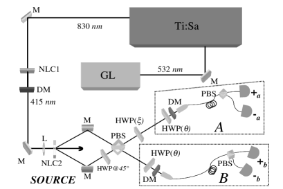
Figure 1: Experimental set-up: the time-compensated source of photon pairs in the state $|\varphi(\xi)\rangle_{ab}$ is composed of a type II nonlinear crystal (NLC2), pumped by the pulsed laser system (LD, Ti:Sa and NLC1), of a polarizing beam splitter (PBS), and of half-wave plates (HWP). Photons $a$ and $b$ of each pairs are directed towards the corresponding detection apparatuses (”A” and ”B”) to perform the local measurements, by means of HWPs, dichroic mirrors (DM) fiber couplers, fibers integrated PBS, single-photon detectors. M mirror, L lens

Given this theoretical breakthrough, Cabello’s proposal cabellos of an experiment to test the behavior of the quantum correlations, is of straightforward interest, and in this paper we perform this experiment by the setup depicted in Fig. 1. In this scheme, the source of pulsed parametric down-conversion (PDC) -to date the most easy method to generate two-particle quantum correlation- is obtained by a 3 mm length BBO nonlinear crystal (NLC2) with an average pumping power of 20 mW. Ultrashort pump pulses (160 fs) at 415 nm are generated from the second harmonic (NLC1) of a mode-locked Ti-Sapphire with repetition rate of 76 MHz pumped by 532 nm green laser. PDC degenerate photon pairs at 830 nm are generated by a non-collinear type II phase matching for a 3.4^∘ emission angle, providing eventually a polarization entanglement, i.e. the singlet state $|\psi^{-}\rangle_{ab}=2^{-1/2}(|H\rangle_{a}|V\rangle_{b}-|V\rangle_{a}|H\rangle_{b})$ kwiat2 , when time-compensated PDC scheme is applied kimgrice . To realize the set of entangled states $|\varphi(\xi)\rangle_{ab}$ in Eq. (LABEL:fi) an half-wave plate (HWP) on the channel $b$ is used to rotate the polarization of photon $b$ of an angle $\xi-\pi/2$.

The local measurements on photon $a$ and $b$ are preformed by identical apparatuses composed of open-air fiber couplers collecting the PDC in single-mode optical fibers. HWPs before the fiber coupler together with fiber-integrated polarizing beam splitters (PBSs) project photons in the polarization basis $\{|s(\alpha)\rangle=\cos(\alpha/2)|H\rangle+\sin(\alpha/2)|V\rangle,|s^{\bot}(\alpha)\rangle\ =\sin(\alpha/2)|H\rangle-\cos(\alpha/2)|V\rangle\}$. Photons at the output ports of the PBSs are detected by fiber coupled photon counters (Perkin-Elmer SPCM-AQR-14) disc . Dichroic mirror are placed in front of the fiber couplers to reduce straylight, and optimization of single-mode fiber collection, yielding the highest final visibility in the experiment, is guaranteed by a proper engineering of pump and collecting mode in the experimental conditions fabiogianni .

The Filipp and Svozil local observables can be rewritten for the chosen polarization basis $\{|s(\alpha)\rangle,|s^{\bot}(\alpha)\rangle\}$ as

$$\widehat{O}(\alpha)=|s(\alpha)\rangle\langle s(\alpha)|-|s^{\bot}(\alpha)\rangle\langle s^{\bot}(\alpha)|;$$

and thus, the correlation function $\langle\widehat{O}_{a}(\alpha)\widehat{O}_{b}(\beta)\rangle$ in terms of coincidence detection probabilities, $p_{x_{a},y_{b}}(\alpha,\beta,\xi)$ ($x,y=+,-$), as

$$\langle\widehat{O}_{a}(\alpha)\widehat{O}_{b}(\beta)\rangle=p_{+_{a},+_{b}}(\alpha,\beta,\xi)+p_{-_{a},-_{b}}(\alpha,\beta,\xi)-p_{+_{a},-_{b}}(\alpha,\beta,\xi)-p_{-_{a},+_{b}}(\alpha,\beta,\xi)$$

where

$$p_{+_{a},+_{b}}(\alpha,\beta,\xi) = |\langle\varphi(\xi)_{ab}|s(\alpha)\rangle_{a}|s(\beta)\rangle_{b}|^{2},$$

$$p_{-_{a},-_{b}}(\alpha,\beta,\xi) = |\langle\varphi(\xi)_{ab}|s^{\bot}(\alpha)\rangle_{a}|s^{\bot}(\beta)\rangle_{b}|^{2},$$

$$p_{+_{a},-_{b}}(\alpha,\beta,\xi) = |\langle\varphi(\xi)_{ab}|s(\alpha)\rangle_{a}|s^{\bot}(\beta)\rangle_{b}|^{2},$$

$$p_{-_{a},+_{b}}(\alpha,\beta,\xi) = |\langle\varphi(\xi)_{ab}|s^{\bot}(\alpha)\rangle_{a}|s(\beta)\rangle_{b}|^{2}.$$

$p_{x_{a},y_{b}}(\alpha,\beta,\xi)$ are normalized in terms of the number of coincident counts:

$$p_{x_{a},y_{b}}(\alpha,\beta,\xi)=\frac{N_{x_{a},y_{b}}(\alpha,\beta,\xi)}{\begin{array}[]{c}[N_{+_{a},+_{b}}(\alpha,\beta,\xi)+N_{+_{a},-_{b}}(\alpha,\beta,\xi)+\\ N_{-_{a},+_{b}}(\alpha,\beta,\xi)+N_{-_{a},-_{b}}(\alpha,\beta,\xi)]\end{array}}$$ (6)

where $N_{x_{a},y_{b}}(\alpha,\beta,\xi)$ is the number of coincidences measured by the pair of detectors $x_{a},\,y_{b}$ for $a$ and $b$ detection apparatuses projecting photons in the above described polarization basis. Coincident counts are measured by an Elsag prototype of four-channel coincident circuit elsag1 ; elsag2 . Single-counts and coincidences are counted by a National Instruments disc sixteen channels counter plug-in PC card.

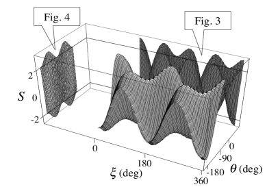
Figure 2: Plot of the CHSH parameter $S$ versus $\xi$ and $\theta$. ”Fig. 3” and ”Fig. 4” indicates the projection of the curve $S$ along $\theta$ and $\xi$ directions, respectively.

In Fig. 2 the central surface represents the theoretical value of the CHSH parameter $S$, plotted versus $\theta$ and $\xi$. The other two shadows labelled ”Fig. 3” and ”Fig. 4” are the projections of the surface along $\theta$ and $\xi$, respectively. These shadows highlight the theoretical bounds of $S$ for the different values of $\theta$ and $\xi$.

Fig.s 3 and 4 show highly stable and repeatable $S$ measurement points for many choices of $\theta$ and $\xi$. As so far theoretically reported, the CHSH parameter satisfies Cirel’son’s inequality, and for certain values of $\theta$, there are ranges of $S$ value not attainable by any quantum states.

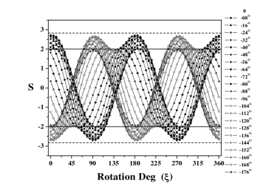
Figure 3: Experimental data: The CHSH parameter $S$ versus $\xi$. Each curves corresponds to a specific choice of $\theta$. Plot points are the measured values of $S$ for any pair of values $\theta$ and $\xi$.

Fig. 3 shows $S$ versus $\xi$ where the classical ($|S|=2$) and the quantum ($|S|=2\sqrt{2}$) limits are indicated. Each curves corresponds to a different value of $\theta$, and these curves are in good qualitative agreement with the theoretical predictions, also in the case of quantum correlation bounds, as can be seen by comparing Fig. 3 with the correspondent shadow of Fig. 2.

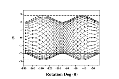
Figure 4: Experimental data: The CHSH parameter $S$ versus $\theta$. Each curves corresponds to a specific choice of $\xi$. Plot points are the measured values of $S$ for any pair of values $\theta$ and $\xi$.

The main thrust of the paper is reported in Fig. 4, where the measured values of $S$ are plotted versus $\theta$ and the various curves are associated to different values of the parameter $\xi$. The thicker curves correspond to the theoretically predicted $S$ bounds cabellos . There is a good qualitative and also quantitative agreement between theoretical and experimental bounds, even if the experimental upper (lower) bounds stands slightly below (above) the theoretical predictions. These effects are, as usual, imputable to noise and imperfections associated to the polarization preservation and measurement of same setup components, namely HWPs, PBSs, and fibers pranostro . In fact, the discrepancy between the theoretical and the experimental results observed in this experiment is confirmed by an equivalent noise level as verified during the alignment process, e.g. at specific trivial angle settings of the polarizers.

In conclusion we performed the appealing experiment proposed in Ref. cabellos , to investigate the bounds of the quantum correlation. According to quantum mechanics we did not observe any violation of Cirel’son’s inequality, with the experimental measured bounds in agreement with the predicted ones within the experimental known limitations; thus we can assert that our experimental results confirm the predictions of quantum mechanics.

Despite the fact that there is no plausible theory which helps us to design a state which violates the quantum correlation bounds, we underline that the actual experiment is not able to search for these violation. Quantum mechanics predicts that no quantum state can violate these quantum bounds for any value of $\theta$. To verify, at least partially, this last statement we are working on the design of a new state-source to span portion of the two-qubit-Hilbert space larger than the one identified by Eq. (4).

In our opinion the above described theory and experiment can be of relevance in the big picture of controlling, manipulating, and mapping quantum states, specifically in what this implies in the emerging field of quantum technologies.

We thanks A. Cabello and M. L. Rastello for the encouragement and for helpful suggestions. We are indebted to A. M. Colla, P. Varisco, A. Martinoli, P. De Nicolo, S. Bruzzo, M. Genovese, I. Ruo Berchera. This experiment was carried out in the Quantum Optics Laboratory of Elsag S.p.A., Genova (Italy), within a project entitled ”Quantum Cryptographic Key Distribution” co-funded by the Italian Ministry of Education, University and Research (MIUR) - grant n. 67679/ L. 488.

References

- (1) A. Einstein, B. Podolsky, and N. Rosen, Phys. Rev. 47, 777 (1935).
- (2) D. Bohm, Phys. Rev. 108, 1070 (1957).
- (3) J. Bell, Physics 1, 195 (1964).
- (4) J. F. Clauser, M. A. Horne, A. Shimony, and R. A. Holt, Phys. Rev. Lett. 23, 880 (1969).
- (5) J. F. Clauser, and M. A. Horne, Phys. Rev. D 10, 526 (1974), E. P. Wigner, Am. J. Phys 38, 1005 (1970), J. D. Franson, Phys. Rev. Lett. 62, 2205 (1989), D. M. Greenberger, M. A. Horne, A. Shimony, and A. Zeilinger, Am. J. Phys. 58, 1131 (1990).
- (6) A. Aspect J. Dalibard, and G. Roger, Phys. Rev. Lett. 49, 1804 (1982), Z. Y. Ou, and L. Mandel, Phys. Rev. Lett. 61, 50 (1988), Y. H. Shih, and C. O. Alley, Phys. Rev. Lett. 61, 2921 (1988), J. G. Rarity, and P. R. Tapster, Phys. Rev. Lett. 64, 2495 (1990), P. G. Kwiat, A. M. Steinberg, and R. Y. Chiao, Phys. Rev. A 47, R2472 (1993), W. Tittel, J. Brendel, H. Zbinden, and N. Gisin, Phys. Rev. Lett. 81, 3563 (1998), G. Weihs, T. Jennewein, C. Simon, H. Weinfurter, and A. Zeilinger, Phys. Rev. Lett. 81, 5039 (1998), M. A. Rowe et al., Nature 409, 791 (2001).
- (7) B. S. Cirel’son, Lett. Math. Phys. 4, 93 (1980).
- (8) A. Cabello, e-print arXiv:quant-ph/0309172 v1.
- (9) R. F. Werner, and M. M. Wolf, Phys. Rev. A 64, 032112 (2001), A. Masanes, e-print arXiv:quant-ph/0309137 v1.
- (10) S. Filipp, and K. Svozil, e-print arXiv:quant-ph/0306092 v1.
- (11) P. G. Kwiat, K. Mattle, H. Weinfurter, A. Zeilinger, A. V. Sergienko and Y. Shih, Phys. Rev. Lett. 75, 4337 (1995).
- (12) Y.-H. Kim, S. P. Kulik, M. V. Chekhova, W. P. Grice, and Y. Shih, Phys. Rev. A 67, 010301(R) (2003).
- (13) Certain trade names and company products are mentioned in the text or identified in an illustration in order to adequately specify the experimental procedure and equipment used. In no case does such identification imply recommendation or endorsement by the Istituto Elettrotecnico Nazionale G. Ferraris, or by ELSAG S.p.A., nor does it imply that the products are necessarily the best available for the purpose.
- (14) F. A. Bovino, P. Varisco, A. M. Colla, G. Castagnoli, G. Di Giuseppe, A. V. Sergienko, Opt. Commun. (to appear).
- (15) P. Varisco, Tecniche e Circuiti di Coincidenza, ELSAG Tec. Rep. HK4CKDS G10, (2002).
- (16) P. Varisco, Software di acquisizione dati, ELSAG Tec. Rep. HK4CKDS G08, (2002).
- (17) S. Castelletto, I. P. Degiovanni, M. L. Rastello, Phys. Rev. A 67, 022305 (2003).