Proposed Experiment to Test the Bounds of Quantum Correlations

Abstract

The combination of quantum correlations appearing in the Clauser-Horne-Shimony-Holt inequality can give values between the classical bound, $2$, and Tsirelson’s bound, $2\sqrt{2}$. However, for a given set of local observables, there are values in this range which no quantum state can attain. We provide the analytical expression for the corresponding bound for a parametrization of the local observables introduced by Filipp and Svozil, and describe how to experimentally trace it using a source of singlet states. Such an experiment will be useful to identify the origin of the experimental errors in Bell’s inequality-type experiments and could be modified to detect hypothetical correlations beyond those predicted by quantum mechanics.

Quantum mechanics is the most accurate and complete description of the world known. This belief is supported by thousands of experiments. Particularly, it is widely agreed that, leaving aside some loopholes Aspect99 ; Grangier01 , no local-realistic theory of the type suggested by Einstein, Podolsky, and Rosen EPR35 is compatible with the experimental results showing violations of Bell’s inequalities Bell64 and “good agreement” with the predictions of quantum mechanics ADR82 ; SA88 ; OM88 ; OPKP92 ; TRO94 ; KMWZSS95 ; TBZG98 ; WJSHZ98 ; RKVSIMW01 .

On the other hand, current technology allows us to perform Bell’s inequality-type experiments with relative ease. Here we propose using this possibility for a systematic test of the bounds of quantum correlations. The benefits of this proposal, apart from confirming quantum mechanics, would be to help us to identify and discriminate between two sources of possible errors in Bell’s inequality-type experiments and to describe a method for searching for hypothetical correlations beyond those predicted by quantum mechanics.

To introduce the bounds of quantum correlations, let us consider a high number of copies of systems of two distant particles prepared in an unspecified way. Let $A$ and $a$ ($B$ and $b$) be physical observables taking values $-1$ or $1$ referring to local experiments on particle $I$ ($II$). Here we shall initially assume that the particles have spin-$\frac{1}{2}$, and that $A$ is a spin measurement along the direction represented by the unit ray $\vec{A}$, etc. Fine Fine82a proved (see also GM82 ; Fine82b ; WW01 ) that a set of four correlation functions $X_{0}=\langle AB\rangle$, $X_{1}=\langle Ab\rangle$, $X_{2}=\langle aB\rangle$, $X_{3}=\langle ab\rangle$ can be attained by a local-realistic theory (i.e., a theory in which the local variables of a particle determine the results of local experiments on this particle) if and only if they satisfy the following eight Clauser-Horne-Shimony-Holt (CHSH) inequalities CHSH69 :

$$-2\leq X_{i}+X_{(i+1){\rm mod}\,4}+X_{(i+2){\rm mod}\,4}-X_{(i+3){\rm mod}\,4}\leq 2,$$ (1)

where $i=0,1,2,3$ and $(p+q){\rm mod}\,4$ means addition of $p$ and $q$ modulo $4$.

On the other hand, Tsirelson Tsirelson80 ; Landau87 showed that, for any quantum state $\rho$, the corresponding quantum correlations, $x_{0}=\langle AB\rangle_{\rho}$, $x_{1}=\langle Ab\rangle_{\rho}$, $x_{2}=\langle aB\rangle_{\rho}$, $x_{3}=\langle ab\rangle_{\rho}$ must satisfy

$$-1 \leq x_{i}\leq 1,$$

$$-2\sqrt{2} \leq x_{i}+x_{(i+1){\rm mod}\,4}+x_{(i+2){\rm mod}\,4}$$ (2)

$$-x_{(i+3){\rm mod}\,4}\leq 2\sqrt{2}.$$

Quantum mechanics predicts violations of the CHSH inequalities (1) up to $2\sqrt{2}$. Such violations can be obtained with pure CHSH69 or mixed states BMR92 .

However, inequalities (2) are only a necessary but not sufficient condition for the correlations to be attainable by quantum mechanics. To illustrate this point, let us consider a set of four numbers $Y_{i}$, such that they satisfy (2) but not (1); that is, their CHSH combinations lie between Bell’s classical bound and Tsirelson’s bound. The question is: Are there always a quantum state $\rho$ and four local observables $A$, $a$, $B$, and $b$ such that $Y_{i}=x_{i}$? The answer is no; certain sets of correlations cannot be reached by any quantum state and any set of local observables. If quantum mechanics is correct, this means that certain sets of expectation values will never be found experimentally. Therefore, the notion of superquantum correlations (i.e., correlations beyond those predicted by quantum mechanics) is not only restricted to sets of correlations such that the value of their CHSH operator is between $2\sqrt{2}$ and $4$ (the maximum possible value for the CHSH operator) PR94 , but it also covers some sets of correlations whose CHSH operator is between $2$ and $2\sqrt{2}$.

Uffink’s quadratic inequalities Uffink02 provide a more restrictive necessary (but still not sufficient) condition for the correlations to be attainable by quantum mechanics. The necessary and sufficient condition for a set of four numbers to be reached by quantum mechanics was found by Landau Landau88 and Tsirelson Tsirelson93 , and has been rediscovered by Masanes Masanes03 . Four numbers $y_{i}$ can be reached by a quantum state and some local observables (i.e., $y_{i}=x_{i}$) if and only if they satisfy a the following eight inequalities:

$$\!\!\!\!-\pi\! \leq \!\arcsin{y_{i}}+\arcsin{y_{(i+1){\rm mod}\,4}}$$ (3)

$$\!+\arcsin{y_{(i+2){\rm mod}\,4}}-\arcsin{y_{(i+3){\rm mod}\,4}}\leq\pi.$$

The inequalities (3) define the whole set of quantum correlations but do not provide a practical characterization of its bounds.

A different approach has been proposed by Filipp and Svozil FS03 . They define the quantum bounds as follows: Let us choose several particular sets of local observables $\{A_{j},a_{j},B_{j},b_{j}\}$; let us use a computer to randomly generate a high number of arbitrary quantum states $\{\rho_{k}\}$, and calculate for all of them the value of the CHSH operator defined as

$${\rm CHSH}=\langle AB\rangle_{\rho}+\langle Ab\rangle_{\rho}+\langle aB\rangle_{\rho}-\langle ab\rangle_{\rho}.$$ (4)

The maximal and minimal values obtained are a numerical estimation of the bounds of the quantum correlations. Given the way in which the bounds have been constructed, for a given set of local observables no quantum state (and, presumably, no other preparation of physical systems) gives values outside these bounds. A suitable parametrization of both the set of local observables and the set of initial states yields to an analytical expression of the bound of quantum correlations. However, Filipp and Svozil’s results are limited to a computer exploration of these bounds. They conclude by saying that “the exact analytical geometries of quantum bounds remain unknown” FS03 . In this Letter, we provide the analytical expression of the bounds of the quantum correlations using Filipp and Svozil’s parametrization for the local observables. We then use this analytical expression to describe how to experimentally trace this bound. This experimental verification will require a set of Bell’s inequality-type tests, each of them using a particular set of local observables and a particular initial state. Both the local observables and the initial state will depend on a single parameter $\theta$.

A suitable parametrization of the local observables and the initial states should reflect the essential features of the bound of quantum correlations: For every possible value of the parameters, the CHSH operator should give values in the range $[2,2\sqrt{2}]$ (that is, between the classical Bell’s bound and Tsirelson’s bound), but it will cover only a subset of the whole. The area of this subset divided by the area of the whole set should reflect the ratio between the difference between the hypervolume of the convex set of quantum correlations defined by (3) and that of the classical correlation polytope (a four-dimensional octahedron) Pitowsky86 ; Pitowsky89 defined by (1) divided by the difference between the hypervolume of the set defined by (2) (which is the intersection of a bigger four-dimensional octahedron and a four-dimensional cube) and that of the classical correlation polytope. Another important property is that quantum bounds can always be attained using a suitably chosen maximally entangled state. For practical reasons, it would be interesting that the parametrization use as few parameters as possible.

Filipp and Svozil FS03 choose the following set of local observables which depends on a single parameter,

$$A = \cos(2\theta)\sigma_{z}+\sin(2\theta)\sigma_{x},$$ (5)

$$B = \cos(\theta)\sigma_{z}+\sin(\theta)\sigma_{x},$$ (6)

$$a = \sigma_{z},$$ (7)

$$b = \cos(3\theta)\sigma_{z}+\sin(3\theta)\sigma_{x},$$ (8)

where $0\leq\theta\leq\pi$, and $\sigma_{z}$ and $\sigma_{x}$ are the usual Pauli matrices.

Figure 1: Values of the CHSH operator for the maximally entangled states $|\phi(\xi)\rangle=\cos\xi|\phi^{+}\rangle+\sin\xi|\psi^{-}\rangle$, for $0\leq\xi<2\pi$, for the local measurements (5)–(8) parametrized by $\theta$. The analytical expression of the quantum bound (thick line) is given by (10). Given a particular set of local measurements (i.e., a particular value of $\theta$), the quantum bound is reached by the maximally entangled states with $\xi(\theta)$ given by (12). No other quantum state (and, presumably, no other preparation of physical systems) gives values outside these bounds. Dashed lines represent Bell’s classical bounds ($\pm 2$) and Tsirelson’s bounds ($\pm 2\sqrt{2}$).

To obtain the analytical expression of the corresponding quantum bound $F(\theta)$, it is useful to remember that, for each $\theta$, the bound of quantum correlations can be reached by a maximally entangled state. For the Filipp and Svozil parametrization, a suitable set of maximally entangled states turns out to be

$$|\varphi(\xi)\rangle=\cos\xi\,|\phi^{+}\rangle+\sin\xi\,|\psi^{-}\rangle,$$ (9)

where $0\leq\xi<2\pi$. In Fig. 1 we show the values of the CHSH operator for several of these states. If, for a given $\theta$, we calculate the maximum and minimum values of the CHSH operator for the states $|\varphi(\xi)\rangle$, we obtain the analytical expression for the bound numerically estimated in FS03 . The analytical expression of the bound of quantum correlations is

$$F(\theta) = \pm 2\left\{\left[1+\sin^{2}(2\theta)\right]^{-1/2}\right.$$ (10)

$$\left.+g(\theta)\sin(2\theta)\left[1+{2\over\cos(4\theta)-3}\right]^{1/2}\right\},$$

where

$$g(\theta)=\left\{{\matrix{{1}&{\rm if}&{0\leq\theta<\pi/2}\cr{-1}&{\rm if}&{\pi/2\leq\theta\leq\pi.}}}\right.$$ (11)

This bound is represented by a thick line in Fig. 1.

The next problem is how to experimentally achieve this bound. Given a particular set of local measurements (i.e., a particular value of $\theta$), which state should we prepare to obtain the quantum upper and lower bounds? It can be easily seen that the quantum upper bound is reached by the maximally entangled states $|\varphi(\xi)\rangle$ given by (9), taking

$$\xi=\frac{1}{2}\left(\theta-g(\theta)\arccos\left\{\left[1+\sin^{2}(2\theta)\right]^{-1/2}\right\}\right).$$ (12)

The quantum lower bound is obtained just by introducing a minus sign inside the arc cosine in (12). No other quantum state gives values outside these bounds.

For practical purposes, it is useful to realize that the required initial states can be prepared using a source of singlet states

$$|\psi^{-}\rangle={1\over\sqrt{2}}\left(|01\rangle-|10\rangle\right),$$ (13)

and applying a suitable unitary transformation $U(\theta)$ to particle $I$. This follows from the fact that, for any $\xi$,

$$|\varphi(\xi)\rangle=U(\xi)\otimes{\sf 1\rule{0.43057pt}{6.54443pt}\rule[-0.08612pt]{1.29167pt}{0.43057pt}}\,|\psi^{-}\rangle,$$ (14)

where

$$U(\xi)=\left({\matrix{{\sin\xi}&{-\cos\xi}\cr{\cos\xi}&{\sin\xi}\cr}}\right),$$ (15)

and ${\sf 1\rule{0.43057pt}{6.54443pt}\rule[-0.08612pt]{1.29167pt}{0.43057pt}}$ is the identity matrix. Therefore, the setup required to test the quantum bound $F(\theta)$ is illustrated in Fig. 2. It consists of a source of two-qubit singlet states $|\psi^{-}\rangle$, a unitary operation $U(\theta)$ [given by (15) and (12)] on qubit $I$, and the local measurements $A(\theta)$ [given by (5)] and (alternatively) $a(\theta)$ [given by (7)] on qubit $I$, and $B(\theta)$ [given by (6)] and (alternatively) $b(\theta)$ [given by (8)] on qubit $II$. A systematical test of the bounds of quantum correlations can be achieved by performing $N$ Bell’s inequality-type tests, each for a particular value of $\theta$ (i.e., for a particular choice of local observables $A(\theta)$, $a(\theta)$, $B(\theta)$, and $b(\theta)$, and a particular state $|\varphi(\theta)\rangle$), covering the range $0\leq\theta\leq\pi$.

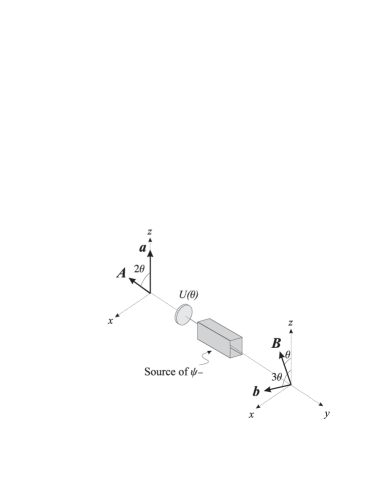
Figure 2: Scheme of the experiment to test the bounds of quantum correlations. It consists of a source of two-qubit singlet states $|\psi^{-}\rangle$, a unitary operation $U(\theta)$ [given by (15) and (12)] on qubit $I$, and the local measurements $A(\theta)$ [given by (5)] and (alternatively) $a(\theta)$ [given by (7)] on qubit $I$, and $B(\theta)$ [given by (6)] and (alternatively) $b(\theta)$ [given by (8)] on qubit $II$. The experiment consists of a set of $N$ Bell’s inequality-type tests for $N$ different values of $\theta$ in the range $[0,\pi]$.

In order to make the CHSH inequality (1) useful for real experiments, it is common practice to translate it into the language of joint probabilities. This leads to the Clauser-Horne (CH) inequality CH74 ; Mermin95 :

$$-1 \leq P\left(A=1,B=1\right)-P\left(A=1,b=-1\right)$$ (16)

$$+P\left(a=1,B=1\right)+P\left(a=1,b=-1\right)$$

$$-P\left(a=1\right)-P\left(B=1\right)\leq 0.$$

It can be easily seen that the bounds $l$ of the CHSH inequality (1) are transformed into the bounds $(l-2)/4$ of the CH inequality (16). Therefore, the local-realistic bound in the CH inequality is 0, and Tsirelson’s bound is $(\sqrt{2}-1)/2$. Analogously, if we calculate the values of the CH operator

$${\rm CH} = P_{\rho}\left(A=1,B=1\right)-P_{\rho}\left(A=1,b=-1\right)$$ (17)

$$+P_{\rho}\left(a=1,B=1\right)+P_{\rho}\left(a=1,b=-1\right)$$

$$-P_{\rho}\left(a=1\right)-P_{\rho}\left(B=1\right),$$

for the states $|\varphi(\xi)\rangle$, we obtain a figure which looks like Fig. 1 but has a different scale in the vertical axis {i.e., instead of points with coordinates $(\theta,{\rm CHSH})$, we obtain points with coordinates $\left[\theta,({\rm CHSH}-2)/4\right]$}.

This systematic test of the bounds of quantum correlations can be performed with current technology. A physical system particularly suitable for its implementation consists of pairs of photons entangled in polarization produced by degenerate type-II parametric down-conversion KMWZSS95 ; WJSHZ98 . In this system, the role of spin observables is played by polarization observables which are particularly adequate due to the availability of high efficiency polarization-control elements and the relative insensitivity of most materials to birefringent thermally induced drifts. An essential advantage of this system is that it allows Bell’s inequality-type tests under strict space-like separations WJSHZ98 (however, current detector efficiencies do not allow these experiments to elude the so-called detection loophole Grangier01 ).

Apart from providing a systematical way to experimentally verify set of extreme nonclassical predictions of quantum mechanics, two kind of benefits are expected from the proposed experiment.

Identifying the source of experimental errors in tests of Bell’s inequalities.—Since the Hilbert space structure of quantum mechanics is not used in the derivation of Bell’s inequalities, the main conclusion of an experimental violation of a Bell’s inequality is clear: The experimental results are incompatible with local realism. The role of quantum mechanics in a test of Bell’s inequalities is to tell us which physical system we should prepare and in which directions we should orientate our polarizers or Stern-Gerlach devices. However, quantum mechanics does not only tell us this; it also predicts a specific result for the experiment. The point is that this specific prediction relies on some additional assumptions. Some of these assumptions are related to the inefficiencies of our preparations and detectors. Other assumptions concern the adequacy of the quantum-mechanical description of the experiment. The failure of each of these two kinds of assumptions has a different effect on the results. For instance, if the state we have prepared is a Werner state Werner89 such as $\rho=(1-\epsilon)|\psi^{-}\rangle\langle\psi^{-}|+\epsilon{\sf 1\rule{0.43057pt}{6.54443pt}\rule[-0.08612pt]{1.29167pt}{0.43057pt}}/4$ with $0<\epsilon\ll 1$, instead of $|\psi^{-}\rangle$, then the quantum prediction for the proposed experiment is not $F(\theta)$ given by (10), but a curve very close to $F(\theta)$ comprised between the quantum bounds. In other words, in this case the distance between the theoretical prediction assuming the $|\psi^{-}\rangle$ and the experimental result is not significatively sensitive to the value of parameter $\theta$. However, if we have assumed that the measured local observables are accurately described by a two-dimensional Hilbert space, but that a more adequate description would require a higher dimensional Hilbert space then, even if both quantum predictions were similar for some value of $\theta$ and both are comprised between the quantum bounds, the distance between them will be very sensitive to the value of $\theta$.

Searching for correlations beyond those predicted by quantum mechanics.—The proposed experiment can be modified to search for hypothetical correlations beyond those predicted by quantum mechanics (i.e., superquantum correlations in the extended sense mentioned above). We do not have any plausible theory which predicts these correlations and helps us design an experiment showing violations of the inequalities (3). However, by the very definition of the bounds $F(\theta)$, for a given set of local observables, no quantum state can give values outside the bounds $F(\theta)$. To verify this for any fixed set of alternative local observables, we can randomly modify the state emitted by the source. Quantum mechanics predicts that there are no results outside these bounds. The existence of experimental results outside these bounds would mean that there are procedures for preparing physical systems which are not described by any quantum state and, therefore, that quantum mechanics is incomplete.

I thank M. Bourennane, L. Masanes, and H. Weinfurter for helpful discussions, I. Pitowsky and B. S. Tsirelson for references, and the Spanish Ministerio de Ciencia y Tecnología Grant No. BFM2002-02815 and the Junta de Andalucía Grant No. FQM-239 for support.

References

- (1) A. Aspect, Nature (London) 398, 189 (1999).
- (2) P. Grangier, Nature (London) 409, 774 (2001).
- (3) A. Einstein, B. Podolsky, and N. Rosen, Phys. Rev. 47, 777 (1935).
- (4) J.S. Bell, Physics (Long Island City, NY) 1, 195 (1964).
- (5) A. Aspect, J. Dalibard, and G. Roger, Phys. Rev. Lett. 49, 1804 (1982).
- (6) Y.H. Shih and C.O. Alley, Phys. Rev. Lett. 61, 2921 (1988).
- (7) Z.Y. Ou and L. Mandel, Phys. Rev. Lett. 61, 50 (1988).
- (8) Z.Y. Ou, S.F. Pereira, H.J. Kimble, and K.C. Peng, Phys. Rev. Lett. 68, 3663 (1992).
- (9) P.R. Tapster, J.G. Rarity, and P.C.M. Owens, Phys. Rev. Lett. 73, 1923 (1994).
- (10) P.G. Kwiat, K. Mattle, H. Weinfurter, A. Zeilinger, A.V. Sergienko, and Y. Shih, Phys. Rev. Lett. 75, 4337 (1995).
- (11) W. Tittel, J. Brendel, H. Zbinden, and N. Gisin, Phys. Rev. Lett. 81, 3563 (1998).
- (12) G. Weihs, T. Jennewein, C. Simon, H. Weinfurter, and A. Zeilinger, Phys. Rev. Lett. 81, 5039 (1998).
- (13) M.A. Rowe, D. Kielpinski, V. Meyer, C.A. Sackett, W.M. Itano, C. Monroe, and D.J. Wineland, Nature (London) 409, 791 (2001).
- (14) A. Fine, Phys. Rev. Lett. 48, 291 (1982).
- (15) A. Garg and N.D. Mermin, Phys. Rev. Lett. 49, 242 (1982).
- (16) A. Fine, Phys. Rev. Lett. 49, 243 (1982).
- (17) R.F. Werner and M.M. Wolf, Phys. Rev. A 64, 032112 (2001).
- (18) J.F. Clauser, M.A. Horne, A. Shimony, and R.A. Holt, Phys. Rev. Lett. 23, 880 (1969).
- (19) B.S. Tsirelson, Lett. Math. Phys. 4, 93 (1980).
- (20) L.J. Landau, Phys. Lett. A 120, 54 (1987).
- (21) S.L. Braunstein, A. Mann, and M. Revzen, Phys. Rev. Lett. 68, 3259 (1992).
- (22) S. Popescu and D. Rohrlich, Found. Phys. 24, 379 (1994).
- (23) J. Uffink, Phys. Rev. Lett. 88, 230406 (2002).
- (24) L.J. Landau, Found. Phys. 18, 449 (1988).
- (25) B.S. Tsirelson, Hadronic J. Supplement 8, 329 (1993).
- (26) L. Masanes, quant-ph/0309137.
- (27) S. Filipp and K. Svozil, quant-ph/0306092 [Phys. Rev. Lett. (to be published)].
- (28) I. Pitowsky, J. Math. Phys. 27, 1556 (1986).
- (29) I. Pitowsky, Quantum Probability-Quantum Logic (Springer, Berlin, 1989).
- (30) J.F. Clauser and M.A. Horne, Phys. Rev. D 10, 526 (1974).
- (31) N.D. Mermin, Ann. N. Y. Acad. Sci. 755, 616 (1995).
- (32) R.F. Werner, Phys. Rev. A 40, 4277 (1989).