Optical Bistability and Collective Behavior of Atoms trapped in a High-Q Ring Cavity

Abstract

We study the collective motion of atoms confined in an optical lattice operating inside a high finesse ring cavity. A simplified theoretical model for the dynamics of the system is developed upon the assumption of adiabaticity of the atomic motion. We show that in a regime where the light shift per photon times the number of atoms exceeds the line width of the cavity resonance, the otherwise tiny retro-action of the atoms upon the light field becomes a significant feature of the system, giving rise to dispersive optical bistability of the intra–cavity field. A solution of the complete set of classical equations of motion confirms these finding, however additional non-adiabatic phenomena are predicted, as for example self–induced radial breathing oscillations. We compare these results with experiments involving laser–cooled ⁸⁵Rb atoms trapped in an optical lattice inside a ring cavity with a finesse of $1.8\times 10^{5}$. Temperature measurements conducted for moderate values of the atom–cavity interaction demonstrate that intensity–noise induced heating is kept at a very low level, a prerequisite for our further experiments. When we operate at large values of the atom–cavity interaction we observe bistability and breathing oscillations in excellent agreement with our theoretical predictions.

I Introduction

Atoms regularly spaced in optical lattices are a widely studied model system of quantum optics Gri:00 which receives growing attention also from other areas of physics ranging from the fields of condensed matter Jak:00 to quantum information processing Cal:00 . Magneto–optic trapping techniques typically provide optical lattices with an average inter–atomic distance of several microns, where dipole–dipole or spin interactions are negligible. While in this case the atomic dynamics is well understood it appears to be of limited relevance for most conceivable applications. Schemes that provide mutual interactions among the atoms should significantly increase the usefulness of optical lattices. Recently, the formation of optical lattices inside optical resonators has become a subject of extensive research Nag1:03 ; Nag2:03 ; Kru1:03 ; Kru2:03 , because cavity–mediated long range interactions arise, possibly useful for new quantum computing schemes Hem:99 or novel laser cooling methods Doh:97 ; Hor:97 ; Hec:98 ; Cha:03 ; Els:03 which do not rely on cyclic spontaneous emission and thus apply to a wider class of species without degradation to be expected at high densities.

The key to exploiting these new concepts is a profound understanding of the interaction of trapped particles with intra–cavity light fields. For single atoms interacting with only a few photons in cavities with a small mode volume well below 10^-4 mm³ studies have been successfully performed within the last few years Pin:00 ; Hoo:00 . However, in these experiments only a few atoms can be trapped for no more than a few 10 ms due to heating caused by intensity fluctuations of the intra–cavity field. More recently it has been pointed out, that high finesse cavities with large mode volumes exceeding 1 mm³ may be utilized to confine large atomic ensembles with the advantage of far longer trapping times. In this case the high frequency noise components of the intra–cavity light field are significantly suppressed owing to the long lifetime of the photons Nag1:03 . Although operation at large detunings from atomic resonance is required in order to prevent undesirable spontaneous photons, for sufficiently high values of the cavity finesse the strong coupling regime can be reached. In this case the collective interaction strength given by the light shift per photon times the number of trapped particles exceeds the resonance line width of the cavity, and thus the otherwise tiny retro–action of the atoms upon the light field becomes a significant feature of the system.

In this paper we experimentally and theoretically explore the motion of atoms trapped in an optical lattice formed inside a high finesse ring–cavity with a large mode volume. We discuss two different regimes of operation characterized by the strength of the collective atom–cavity coupling. Our observations for moderate coupling strengths show that the experimental challenges introduced by the small cavity resonance bandwidth can be handled and a stable lattice can be produced. At large atom–cavity couplings where the backaction of the atoms upon the lattice potential becomes significant, we find non–linear dynamics of the intra–cavity field and a collective character of the atomic motion. In this regime phenomena like dispersive optical bistability and self–induced breathing oscillations arise. Non–linear dynamics due to optical pumping and saturation has been observed in low–finesse resonators operating close to an atomic resonance Lam:95 . Only recently absorptive optical bistability was observed in a small–volume high–finesse cavity Sau:03 . Our lattice operates far from resonance where optical pumping and saturation are negligible and the atoms merely act as a dispersive medium.

The paper is organized as follows. In Sec. II we present a simple physical picture of the atom–cavity coupling in terms of coherent forward and backward Rayleigh scattering. In Sec. III we briefly discuss the complete set of semiclassical equations of motion of the system. These equations are difficult to solve leading us to develop a simplified but surprisingly accurate model of the complex system dynamics based upon the assumption that the atomic sample adiabatically adjusts to the potential position and depth. A steady–state analysis for the phase and amplitude of the intra–cavity field predicts dispersive bistability. In Sec. IV we discuss the characteristics of our experimental setup. Both cavity modes are externally fed by adjustable amounts of power from a single–mode laser diode. A fast servo–lock keeps the laser frequency in resonance with one of the travelling wave modes of the cavity. The properties of this lock and the implications for parametric heating and expected trapping times are discussed in Sec. V. Noise measurements of the light transmitted through the cavity together with lifetime and temperature measurements of the trapped atomic ensemble show that undesired intra–cavity intensity noise can be maintained at extremely low values despite of the small cavity bandwidth. In Sec. VI we present experiments in the strong coupling regime. For asymmetric pumping of the cavity the unlocked intra–cavity field exhibits distinctive non–linear behavior resulting in bistability of the intra–cavity field. We find an excellent agreement with the predictions of the adiabatic model of Sec. III. In Sec. VII we explore non–adiabatic aspects of the atomic motion. Observations of radial breathing oscillations are discussed and a numerical simulation based on solving the full set of equations of motion is presented.

II Mode Splitting

The interaction of the atomic sample with the intra–cavity light field can be understood in terms of coherent Rayleigh scattering. Consider the two degenerate, mutually counterpropagating, travelling wave modes of a ring resonator (discriminated by indices ($\pm$) in the following) with a common resonance frequency $\omega_{c}$, as depicted in Fig. 1a). Let us add atoms into the common mode volume with a resonance frequency $\omega_{a}>>\omega_{c}$ such that their interaction with the intra–cavity fields has entirely dispersive character. If the atomic sample is homogeneously distributed it will merely give rise to Rayleigh scattering in the forward directions described by a constant index of refraction $n_{\pm}=1+N\,\Delta_{0}/\omega_{c}$, where $\Delta_{0}$ is the light shift per photon and $N$ is the number of atoms. This causes a common frequency shift $N\,\Delta_{0}$ for both modes [Fig. 1b)]. Assume that both modes are externally coupled and an optical lattice is formed inside the cavity which tightly traps the atoms in the Lamb–Dicke regime, where the atomic distribution in each lattice site is confined to a fraction of the optical wavelength. In this case additional backscattering arises, which couples the two counterpropagating modes and lifts their frequency degeneracy giving rise to a frequency splitting $2N\Delta_{0}\,|g|$. The degree of atomic localization is measured by the parameter $g\equiv\frac{1}{N}\sum_{\nu=1}^{N}e^{-i2kz_{\nu}-2(x_{\nu}^{2}+y_{\nu}^{2})/w_{0}^{2}}$, where k is the wave number, $x_{\nu}$, $y_{\nu}$ and $z_{\nu}$ denote the atomic position coordinates, and $w_{0}$ is the mode radius. If there is no statistical correlation between the axial and radial coordinates and the spatial distributions near each lattice site follow a Gaussian, we may write $g=\left(1+4\left(\sigma_{r}/w_{0}\right)^{2}\right)^{-1}exp(-2k^{2}\sigma_{z}^{2})\,exp(-2ikz_{cm})$, i.e., the complex phase scales with the axial center of mass coordinate $z_{cm}\equiv\frac{1}{N}\sum_{\nu=1}^{N}z_{\nu}$ and the modulus is a measure for the axial ($\sigma_{z}$) and radial ($\sigma_{r}$) spread of the atomic sample. Perfect localization corresponds to $|g|=1$, whereas a homogeneous distribution is described by $|g|=0$.

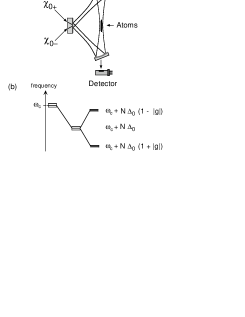
Figure 1: a) Sketch of the experimental setup. Adjustable laser powers $\chi_{0\pm}$ are coupled into the two counterpropagating travelling wave modes of a ring resonator. The power transmitted through the cavity can be detected by a photo diode (PD). b) Mode splitting mechanism (explained in the text).

If the interaction strength $N\,\Delta_{0}$ exceeds the cavity resonance bandwidth, the eigenmodes of the cavity acquire orthogonal standing wave geometries. One of them supports the optical lattice with atoms localized at the antinodes, i.e, the interaction is maximized and the corresponding frequency shift $\omega_{c}+N\Delta_{0}\,\left(1+|g|\right)$ exceeds that found for the travelling wave eigenmodes in presence of a homogeneous atomic sample. The second eigenmode is not externally coupled and its nodes coincide with the atomic center of mass positions thus minimizing interaction. This leads to a reduced shift $\omega_{c}+N\Delta_{0}\,\left(1-|g|\right)$ (Fig.1b). The existence of a second empty eigenmode, blue–detuned with respect to the optical lattice, can be utilized for implementation of a sideband cooling scheme as described in Ref. Els:03 .

It is instructive to consider the change of the indices of refraction $n_{\pm}$ experienced by the travelling wave modes, due to back–scattering. According to the considerations of Ref. Wei:98 (Eq. 7), to first scattering order, the modified refractive indices are given by $n_{\pm}=1+N\,\frac{\Delta_{0}}{\omega_{c}}(1+|g||\frac{\alpha_{\mp}}{\alpha_{\pm}}|)$. Note that $n_{+}$ and $n_{-}$ may differ, if the field amplitudes of the travelling waves $\alpha_{\pm}$ are not equal, e.g., for asymmetric external pumping of the cavity. This gives rise to interesting non–linear dynamics, if back–scattering becomes relevant. A small external pumping asymmetry can yield a relative change of the refractive indices and a corresponding spatial phase shift of the optical standing wave potential. As the laser frequency is kept actively in resonance with say the ($+$)–wave, the ($-$)–wave is tuned slightly out of resonance and the potential well depth decreases. This in turn decreases the degree of localization $|g|$ which reduces the phase shift. As we will see in the following, in a certain parameter range this dynamics provides more than one steady–state, thus giving rise to bistability phenomena.

III Adiabatic Model

We restrict ourselves to the case where the cavity modes support coherent fields with large mean photon numbers interacting with large thermal atomic samples at sufficiently high temperatures such that a classical description of the optical intra–cavity fields and the atomic position and momentum variables is appropriate. Moreover, we assume a large detuning of the pump frequency from the atomic resonance and hence negligible saturation. In this case according to Ref. Gan:00 the following equations describe the time evolution of the complex fields $\alpha_{+}$ and $\alpha_{-}$ for the counterpropagating travelling wave modes scaled to the field per photon

$$\begin{array}[]{ccc}\frac{d}{dt}\left(\begin{array}[]{ccc}\alpha_{+}\\ \alpha_{-}\\ \end{array}\right)=\bf{M}\left(\begin{array}[]{ccc}\alpha_{+}\\ \alpha_{-}\\ \end{array}\right)+\gamma_{0}\left(\begin{array}[]{ccc}\eta_{+}\\ \eta_{-}\\ \end{array}\right)\\ \\ \bf{M}\equiv\left(\begin{array}[]{cc}i\left(\delta_{c}-N\Delta_{0}g_{r}\right)-\gamma_{c}&-iN\Delta_{0}\,g\\ -iN\Delta_{0}\,g^{*}&i\left(\delta_{c}-N\Delta_{0}g_{r}\right)-\gamma_{c}\\ \end{array}\right)\\ \\ g_{r}\equiv\frac{1}{N}\sum_{\nu=1}^{N}e^{-2(x_{\nu}^{2}+y_{\nu}^{2})/w_{0}^{2}}\end{array}$$ (1)

Here $\eta_{+}$ and $\eta_{-}$ are the complex amplitudes of the incoupled light fields, and $\delta_{c}$ denotes the detuning of the incoupled frequency from the resonance frequency $\omega_{c}$ of the empty cavity. The radial bunching parameter $g_{r}$ accounts for the radial position dependence of the atom–light coupling. The diagonal elements of the matrix $\bf{M}$ comprise the forward scattering terms $N\Delta_{0}g_{r}$ which only depend on the degree of radial bunching while the off–diagonal terms which act to couple $\alpha_{+}$ and $\alpha_{-}$ are due to backward scattering and thus involve the localization parameter $g$.

The equations for the momenta $\vec{p}_{\nu}\equiv(p_{x,\nu}$, $p_{y,\nu}$, $p_{z,\nu})$ and the positions $\vec{x}_{\nu}\equiv(x_{\nu},y_{\nu},z_{\nu})$ read

$$\begin{array}[]{ccc}\frac{d}{dt}\vec{p}_{\nu}=\hbar\Delta_{0}\left(\vec{\nabla}\,\,{|\alpha_{+}e^{-ikz}+\alpha_{-}e^{ikz}|}^{2}e^{-2\frac{(x^{2}+y^{2})}{w_{0}^{2}}}\right)\big{|}_{\vec{x}=\vec{x_{\nu}}}\\ \\ \frac{d}{dt}\vec{x}_{\nu}=\frac{1}{m}\vec{p}_{\nu}\end{array}$$ (2)

In total we are concerned with $6N+2$ coupled first–order non–linear differential equations for the $3N$ position and momentum variables, respectively and the two complex field amplitudes for the counter–propagating cavity modes.

In experiments with small bandwidth cavities the frequency of the incoupled laser beam needs to by actively controlled in order to maintain some resonance condition, which allows to couple light into the cavity at all. In our implementation we servo lock the laser frequency to one of the counterpropagating travelling waves (say the (+)–mode) with a technique discussed in detail in V. Here we merely account for the fact that this servo acts to maintain the complex field amplitude $\alpha_{+}$ at a constant value, i.e., $\frac{d}{dt}\alpha_{+}\equiv 0$. Hence, we may combine the two field equations (1) into a single equation for the unlocked mode $\alpha_{-}$

$$\frac{d}{dt}\alpha_{-}=i\frac{\Delta_{0}N}{\varepsilon_{+}}g\alpha_{-}^{2}-\alpha_{-}\gamma_{c}-i\Delta_{0}Ng^{*}\varepsilon_{+}+\varepsilon_{-}\gamma_{c}\,\,\,.$$ (3)

using the abbreviations $\varepsilon_{\pm}\equiv\frac{\gamma_{0}}{\gamma_{c}}\eta_{\pm}$ for the steady state intra–cavity fields in absence of atoms. We may choose $\varepsilon_{\pm}$ to be real without loss of generality, thus fixing the spatial phase of the intra–cavity standing wave for the case when no atoms are present.

For numerical processing and comparison with experiments it is useful to work with unit–free quantities. We hence define scaled fields $a\equiv\alpha_{-}/\sqrt{I_{0}}$ and $\sqrt{\chi_{0\pm}}\equiv\varepsilon_{\pm}/\sqrt{I_{0}}$ with $I_{0}\equiv|\varepsilon_{+}|^{2}+|\varepsilon_{-}|^{2}$ being the sum of the steady state intensities of each travelling wave mode in absence of atoms. Using the scaled time $\tau\equiv\gamma_{c}t$ and the scaled interaction strength $U\equiv\Delta_{0}/\gamma_{c}$ we obtain

$$\frac{d}{d\tau}a=i\frac{UN}{\sqrt{\chi_{0}+}}|g|\hat{g}a^{2}-a-iUN|g|\hat{g}^{*}\sqrt{\chi_{0+}}+\sqrt{\chi_{0-}}\,\,\,.$$ (4)

In order to incorporate the equations of motion for the atomic ensemble into this equation we seek expressions for the complex phase $\hat{g}=g/|g|$ of the localization parameter $g$, which is connected to the atomic center–of–mass coordinate, and the modulus $|g|$ which represents the spatial spread of the atomic sample in each potential well. Therefore, let us consider atoms tightly confined in the optical lattice, such that the time scale of the axial motion is much shorter than the photon life time $(1/2\gamma_{c})^{-1}$ which represents a lower bound for the time scale relevant for changes of the intra–cavity fields. In this case it is reasonable to expect, that the center–of–mass in each potential well of the optical standing wave adiabatically follows the potential minimum, which formally is expressed by the relation $\hat{g}^{*}=a/|a|$. More specifically, we assume that the atomic distribution in the lattice can be described by a sum of Gaussians which are centered at the instantaneous antinodes of the lattice. To evaluate $|g|$ we take into account that there is no statistical correlation between the axial and radial coordinates writing $|g|\approx\langle e^{-i2kz}\rangle\langle e^{-2r^{2}/w_{0}^{2}}\rangle$, where the brackets denote a Gaussian average. These expressions are readily calculated to be $\langle e^{-i2kz}\rangle=e^{-2k^{2}\sigma_{z}^{2}}$ and $\langle e^{-2r^{2}/w_{0}^{2}}\rangle=1/(1+4\sigma_{r}^{2}/w_{0}^{2})$. In order to determine the time evolution of $\sigma_{r}$ and $\sigma_{z}$ we assume that the thermal atomic sample adjusts adiabatically to the potential well depth keeping the Boltzmann factors $\xi_{ax}\equiv k_{B}T_{ax}/\omega_{v,ax}$ and $\xi_{rad}\equiv k_{B}T_{rad}/\omega_{v,rad}$ constant, where $k_{B}$ is the Boltzmann constant and $T_{ax}$ and $T_{rad}$ are the axial and radial temperatures of the sample and $\omega_{v,ax}$ and $\omega_{v,rad}$ denote the axial and radial trap frequencies. By harmonically approximating the potential in axial and radial directions we find $2\sigma_{z}^{2}/k^{2}=k_{B}T(t)/V_{0,ax}=\eta_{ax}\sqrt{a(0)/a(t)}$ and $4\sigma_{r}^{2}/w_{0}^{2}=\eta_{rad}(\sqrt{\chi_{0+}}+|a(0)|)/(\sqrt{\chi_{0+}}+|a(t)|)$, with $\eta_{ax}$ and $\eta_{rad}$ being the ratio between the thermal energy and the potential depth at t=0 for the axial and radial directions, respectively. With these approximations we are in the position to state a single equation for the complex unstabilized electric field amplitude:

$$\frac{d}{d\tau}a\,=\,i\frac{UN}{\sqrt{\chi_{0+}}}\,L(a)\,|a|a\,-\,a\,+{}$$

$$+\,\sqrt{\chi_{0-}}\,-\,iUN\,\sqrt{\chi_{0+}}\,L(a)\,\frac{a}{|a|}\,\,,$$

$$L(a)\equiv e^{-\eta_{ax}\sqrt{\frac{|a_{0}|}{|a|}}}\,\,\frac{1}{1+\eta_{rad}\,\frac{\sqrt{\chi_{0+}}\,+\,|a_{0}|}{\sqrt{\chi_{0+}}\,+\,|a|}}$$ (5)

In this equation all the parameters can be easily obtained by measurements and a numerical integration yields simulations of the intra–cavity field, that can be compared to experimental data. In Sec. VI we will show that despite its simplicity the adiabatic model presented here reproduces our observations very accurately.

We may obtain additional physical insight into the dynamical properties of Eq. (III) by representing the complex field $a$ as $a=|a|e^{i\phi}$ with amplitude $|a|$ and phase $\phi$. Multiplying Eq. (III) by $a^{*}/|a|$ results in separate differential equations for $|a|$ and $\phi$:

$$|a|\frac{d}{d\tau}\phi=UNL(a)(\frac{|a|^{2}}{\sqrt{\chi_{0+}}}-\sqrt{\chi_{0+}})-\sqrt{\chi_{0-}}\sin{\phi}$$ (6)

$$\frac{d}{d\tau}|a|=\sqrt{\chi_{0-}}\cos{\phi}-|a|$$ (7)

Eq. (7) implicates that the amplitude $|a|$ adjusts exponentially to $\sqrt{\chi_{0-}}\cos{\phi}$ determined by the instantaneous value of $\phi$. This happens at the fastest time–scale available inside the cavity, the decay time of the intra–cavity field. Hence, any changes of the intra–cavity field on slower time–scales are governed by the evolution of $\phi$. This lets us adiabatically eliminate Eq. (7) by inserting $|a|=\sqrt{\chi_{0-}}\cos{\phi}$ into Eq. (6), which leads to

$$\frac{d}{d\tau}\phi=\frac{UN}{\sqrt{\chi_{0-}\,\chi_{0+}}}\widetilde{L}(\phi)\left(\chi_{0-}\cos{\phi}-\frac{\chi_{0+}}{\cos{\phi}}\right)$$ (8)

$$-\sqrt{\chi_{0-}}\tan{\phi}$$

$$\widetilde{L}(\phi)\equiv\frac{\exp{\left(-\xi_{ax}\frac{\omega_{R}}{\omega_{V}}\sqrt{\frac{8}{\sqrt{\chi_{0+}\chi_{0-}}\cos{\phi}}}\right)}}{1+\frac{8\xi_{rad}\omega_{R}}{kw_{0}\omega_{V}(\sqrt{\chi_{0+}}+\sqrt{\chi_{0-}}\cos{\phi})}}$$

The localization factor $\widetilde{L}(\phi)$ is rescaled in terms of quantities which remain constant during the time evolution of the system, i.e. the axial and radial Boltzmann factors $\xi_{ax}$ and $\xi_{rad}$, the recoil frequency $\omega_{R}$ the mode radius $w_{0}$ and an effective axial vibrational frequency which is a measure of the total power directed to the cavity. More precisely, $\omega_{V}$ is the axial vibrational frequency corresponding to the optical potential that would arise for symmetric pumping with no atoms inside the cavity, i.e. if $\alpha_{+}=\alpha_{-}=\varepsilon_{+}=\varepsilon_{-}$.

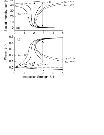
Figure 2: Steady state solutions of Equations (6,7) for the intensity (a) and the phase (b) of the unlocked intra–cavity field for $\chi_{0-}=51\%,50\%,48\%,43\%$ and $38\%$. For $\chi_{0-}<43\%$ only one stable solution exists, while for larger values bistability occurs for $UN$ larger than some value around two. The arrows indicate for the $48\%$–trace, where a jump from one to the other stable solution can occur, if the interaction parameter is tuned.

The dynamical properties of Eq. (III) can be analyzed in terms of its steady state solutions. The steady state values of $\phi$ are obtained as the zeros of the the right hand side of Eq. (8) while the corresponding values of $|a|$ follow directly from Eq. (7). It is particularly instructive to plot these steady state values versus the interaction strength $U\,N$, which can be tuned experimentally. In Fig. 2 this is shown for different degrees of pumping asymmetry, i.e., $\chi_{0-}=51\%,50\%,48\%,43\%$ and $38\%$. In this plot we use our experimental data for $\xi_{ax},\xi_{rad},\omega_{V},k$ and $w_{0}$. For values of $\chi_{0-}<43\%$ only one stable solution exists and the amplitude and phase of the intra–cavity field $a$ are well defined. The situation changes with increasing $\chi_{0-}$. For higher values, e.g. $\chi_{0-}=48\%$ a strong bistability occurs for an interaction strength of $2\lesssim U\,N\lesssim 3$. The upper and lower branch with a positive (negative) slope for the phase (amplitude) are stable, whereas the middle branch is unstable. Experimentally, the interaction strength is readily tuned by a change of the particle number $N$. If one increases $UN$ starting from low values the system will follow the upper branch of the $48\%$–trace in Fig. 2a) until the turning point at $U\,N\approx 3$ is reached, where the intensity suddenly drops to almost zero. On the other hand, when we reduce the number of particles starting from high values, the intensity abruptly jumps from small to high intensity around $U\,N\approx 2$. This hysteresis feature is characteristic for bistable systems. If we approach symmetric pumping (i.e. $\chi_{0-}$ approaches $50\%$ the upper bound of the bistability range (the region on the x–axis between the jumps) moves further out towards infinity whereas the lower bound only slightly increases above two. For $\chi_{0-}\geq 50\%$ the upper bound of the bistability range equals infinity, i.e., the low intensity branch cannot be reached by tuning $U\,N$. In this case a stable optical lattice can be obtained at any value of the interaction strength.

In our analysis we have neglected non–adiabatic aspects of the atomic motion although this is only justified for the axial degrees of freedom which are well confined. Motion along the radial directions occurs on a far slower time scale, and the adiabatic approximation does not hold. A typical non–adiabatic reaction of the radial motion to sudden changes of the potential depth is the excitation of breathing oscillations. Such oscillations would come along with a small oscillatory change of the effective interaction strength. If the system operates deeply inside the bistability regime we may immediately infer from Fig. 2 that small changes of $UN$ with an amplitude well below the extension of the bistability range do not significantly change the intra–cavity intensity. The most drastic reaction of the intensity to a change of $UN$ occurs, if the system is close to the frontier between stable and bistable operation, as in the $43\%$ trace of Fig. 2. In this case we in fact observe oscillations of the intensity which are not predicted by our adiabatic model and which are subject of Sec. VI.

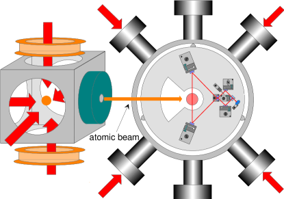
Figure 3: Sketch of the double–MOT system with the resonator placed in the vacuum chamber.

IV Experimental Setup

Preparation of ultracold ⁸⁵Rb atoms is established with a standard double–MOT (magneto–optical trap) setup as depicted in Fig. 3. In a first vacuum chamber a conventional 3D–MOT collects atoms from a Rb dispenser source. One of the retro–reflecting mirrors is provided with a hole, such that an atomic beam is extracted with a flux of $5\cdot 10^{8}$ s^-1 and a mean velocity of 10 m/s. This beam loads a second magneto–optical trap placed in the main UHV chamber with a pressure below $2\cdot 10^{-10}$ mbar. Here we typically trap $5\cdot 10^{8}$ atoms at a temperature of 100 $\mu$K. The implementation of the MOT coils inside the vacuum allows us to switch the magnetic field very rapidly. Contamination emerging via heating of these coils limits the lifetime of the trap to about 2 s.

The experimental implementation of the resonator is also sketched in Fig. 3. In a triangular setup two curved high reflecting mirrors (1.5 ppm transmission) and the flat incoupling mirror (23 ppm transmission) form the high finesse ring cavity with a round trip path length of 97 mm and a free spectral range of 3.1 GHz. The beam waists $w_{0}$ ($1/e^{2}$ mode radius) in sagittal and vertical directions are 134 $\mu$m and 129 $\mu$m, respectively. The beam splitting optics is included in the vacuum to keep the path lengths between the splitter and the incoupling mirror as short as possible. This is favorable because the path length difference influences the spatial phase of the intra–cavity standing wave.

For the trapping light we use an extended cavity grating stabilized diode laser with variable detuning relative to the D2 transition of ⁸⁵Rb. An acoustooptical modulator (AOM) serves as a fast switch and an intensity regulator for the lattice. We analyze the reflected and transmitted light with three avalanche photo diodes.

V Stabilization, parametric heating, trapping time

In order to stabilize the laser diode emission to the cavity resonance, we use a frequency modulation technique (Pound–Drever–Hall) with a servo bandwidth of several MHz. Similarly as in Ref. Sch:01 the fast branch of the feedback control directly applies the PDH–error signal to the injection current of the diode after passing a loop filter, which compensates for frequency–dependent phase shifts on the diode laser chip. With the laser locked to the resonator we can measure the photon lifetime $1/2\gamma_{c}$ = 9.3 $\mu$s corresponding to a finesse of the cavity of F = $1.8\cdot 10^{5}$, a cavity resonance line width of 17 kHz and a mean scattering loss per mirror of 3 ppm.

A sufficiently fast and efficient stabilization is needed to prevent intensity fluctuations of the intra–cavity field which lead to exponential heating of the trapped atoms Sav:97 . In particular, in the case of a small cavity resonance line width tiny frequency deviations are readily converted into intensity fluctuations. Unfortunately, the heating time scales quadratically with the trap frequency, which typically is on the order of a few hundred kHz for the axial direction in a standing wave trap Sav:97 :

$$\dot{W}=\frac{1}{3}\gamma_{a}W+\frac{2}{3}\gamma_{r}W\quad\,\gamma_{a,r}=\pi^{2}\nu_{a,r}^{2}S(2\nu_{a,r})$$ (9)

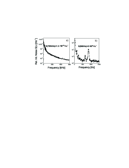
Figure 4: Relative intensity noise power spectrum. a) High frequency part of the spectrum up to 1 MHz, relevant for axial heating b) Low–frequency part of the spectrum responsible for radial heating. The pronounced peak at $\approx$ 850 Hz originates from the turbo pump.

Here W is the mean kinetic energy and $\nu_{a,r}$ are the trap frequencies of the atoms in axial and radial direction, respectively. $S(2\nu)$ denotes the one–sided power spectrum of the fractional intensity noise. The heating rate involves the noise intensity at the second harmonic of the vibrational frequency because parametric excitation is the main source of heating. Here, we assumed that the atomic sample is thermalized resulting in the same mean kinetic energy for all dimensions. Nevertheless, the heating rates for the radial and axial directions may be significantly different. We have measured the intensity fluctuations $S(2\nu)$ by analyzing the transmission through one of the high reflectors. The resulting power spectrum of the relative intensity noise is shown in Fig. 4. For typical trap parameters $\nu_{a}$=350 kHz and $\nu_{r}$=450 Hz we find S(700 kHz)=$1.5\cdot 10^{-13}$ Hz^-1 and S(900 Hz)=$3\cdot 10^{-9}$ Hz^-1 resulting in a heating time (time for an e–fold temperature increase) $\tau_{h}=(1/3\gamma_{a}+2/3\gamma_{r})^{-1}$ exceeding 20 s. This indicates that heating due to intensity noise should not be a limiting factor for experiments with trapping times up to several seconds. The decrease of the intensity noise with 20 dB per decade starting at $\sim$17 kHz is not surprising, because the resonator acts as a low pass filter due to the long photon lifetime. Obviously, the small cavity line width only complicates the stabilization of the intra–cavity field with respect to low noise frequencies, while high noise frequencies are strongly suppressed.

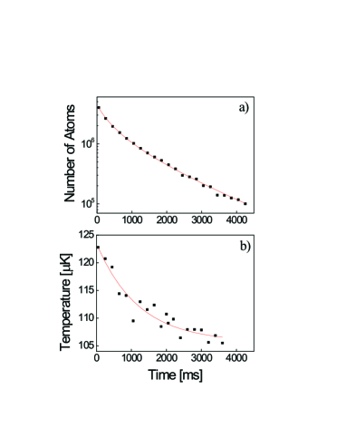
Figure 5: a) Temporal evolution of the trap population determined by fluorescence imaging. The solid line represents a fit to a model which accounts for two–body losses. b) Temperature evolution with time. The solid line shows a fit of Eq.V to the experimental data

Our noise analysis promises trapping times on the order of a few seconds limited merely by background collisions. In order to confirm this prediction we have tuned the optical lattice 7 nm below the D2–line of ⁸⁵Rb, where the collective interaction parameter $U\,N$ is well below unity. In this weak coupling regime we have conducted life time and temperature measurements. We couple a power of 60 $\mu$W into each running wave mode, which is enhanced by a factor of about 70000 to produce a trap depth of 350 $\mu$K corresponding to axial and radial frequencies of 350 kHz and 450 Hz, respectively.

We typically load $4\cdot 10^{6}$ atoms into the lattice with an initial temperature of about 100 $\mu$K. In Fig. 5a) we plot the observed trap population versus time. It shows a non–exponential two–body decay at the beginning with an exponential decay time of 1.7 s representing the main contribution after 500 ms. The solid line is a fit according to a standard trap decay model including a two–body loss term. The two–body losses are explained by evaporation arising due to the relatively high density of $9\cdot 10^{11}$ cm^-3 and the large elastic scattering cross section of ⁸⁵Rb. The expected reduction of the temperature T(t) is shown in Fig. 5b). According to a simple theoretical model presented in Ref. Nag1:03 the temporal temperature evolution follows

$$T(t)=T(0)\,\left(1-\epsilon\,\frac{\beta\rho_{0}}{4\gamma}\left(1-e^{-\gamma t}\right)\right),{}$$

$$\epsilon=\frac{2}{3k_{B}T(0)}\overline{W}-1\,\,,$$ (10)

where $\beta$ is the two–body loss coefficient, $\gamma$ the exponential decay due to background losses and $\rho_{0}$ the peak density in the potential wells. $\overline{W}$ denotes the mean kinetic energy removed by an evaporated particle. The solid line of Fig. 5b) shows a fit to the experimental data by means of Eq. V with $\epsilon=0.23$ used as a fitting parameter, while $\beta$ and $\gamma$ are taken from Fig. 5a) and $\rho_{0}$ is measured directly.

According to Fig. 5b) we do not observe heating at least for the first four seconds of the time evolution that we can follow before the trapped sample disappears. This lets us determine a lower bound for the heating time of about 100 s which is a factor of 4 larger than the value of $\tau_{h}$ taken from the noise measurements. This is not surprising since the temperature is determined for the radial direction, whereas the main contribution to heating originates from the axial direction. The heating rate along the cavity axis is almost two orders of magnitude higher as compared to radial heating. While during the first 500 ms thermalization keeps the axial and radial temperatures locked, this is not so for later times, where the density has decreased beyond the collisional regime and radial heating should slow down significantly.

VI Strong coupling regime

The strong coupling regime is accessed if the collective interaction strength $\Delta_{0}\,N$ exceeds the decay time of the intra–cavity field $\gamma_{c}$ ($UN>1$). In order to keep the spontaneous scattering time of several ms long enough to avoid significant heating, we operate the lattice at $0.7$ nm detuning. This yields a light shift per photon $\Delta_{0}$=0.091 s^-1. Hence with a few $10^{6}$ atoms trapped in the lattice we are able to reach values for $UN$ up to five, well within the strong coupling regime. In the following experiments we have typically applied 5 $\mu$W laser power for each travelling wave mode yielding a trap depth of about 800 $\mu$K for symmetric pumping and in absence of atoms. The corresponding axial vibrational frequency of 500 kHz is sufficiently larger than the 17 kHz cavity bandwidth, i.e., adiabaticity of the axial motion is a well justified assumption. A typical experiment proceeds in three steps. We superimpose the MOT upon the optical lattice for several seconds, before the MOT light is shut off and the atoms remain trapped in the lattice. Finally, the lattice is extinguished and the atoms are given some time to expand ballistically before a fluorescence image of the sample is taken. From the time of flight the radial temperature of the sample is determined. Without ballistic expansion the fluorescence images give information on the spatial distribution of the trapped atoms. We can continuously tune the ratio of powers in the two running wave modes from the case of symmetric pumping $\chi_{0-}=\chi_{0+}$ to one–sided pumping. We lock the laser frequency to only one of the modes, i.e. $\chi_{+}$, and keep its phase and amplitude at a constant value. The power leaking out from the unlocked mode through one of the high–reflectors is detected and used to determine the scaled intensity $\chi_{-}$, which corresponds to $|a|^{2}$ in the theoretical model in Sec. III.

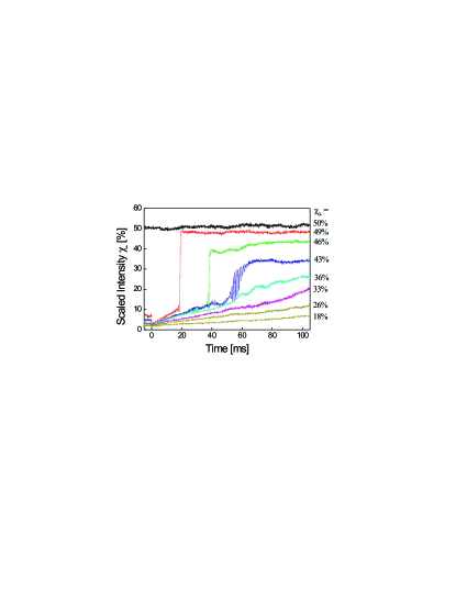
Figure 6: Scaled intensity $\chi_{-}$ for different values of $\chi_{0-}$. The MOT beams are shut off at $t=0\,ms$.

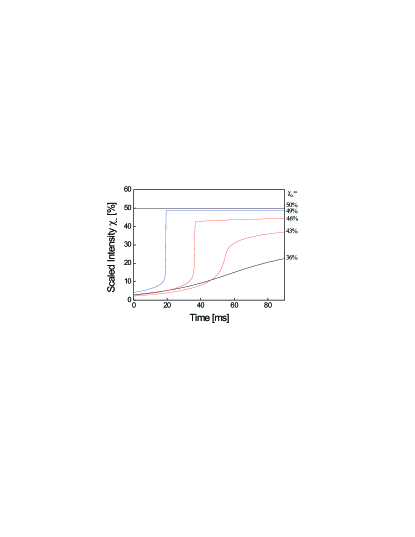
Figure 7: Theoretical simulations of the experimental observations of Fig. 6.

In Fig. 6 we show the time evolution of the scaled intra–cavity intensity $\chi_{-}$ for different types of pumping. The MOT is terminated at t = 0 in this figure. For symmetric pumping ($\chi_{0\pm}$=$50\%$) a stable lattice is formed with equal intensities in each travelling wave mode irrespective of the number of atoms inside the cavity. For values of $\chi_{0-}$ below $50\%$ the situation changes drastically. For an asymmetry of only $1\%$ in favor to the locked mode the intra–cavity intensity $\chi_{-}$ drops to about 10 percent during the MOT phase and to almost zero after shutting off the MOT beams. Subsequently, a slow increase is observed before at about 20 ms the intensity suddenly jumps back to nearly the value $\chi_{0-}$ (the value expected in absence of atoms) with a rise time below a few hundred microseconds. If the power of the unlocked mode is further reduced, the time duration before the jump occurs increases as well as the rise time until the jump completely vanishes for values $\chi_{0-}<40\%$. At a value of ($\chi_{0-}$=$43\%$), where the jump begins to level off, strong oscillations of roughly 1 kHz are observed corresponding to twice the radial vibrational frequency. The traces for asymmetric pumping in Fig. 6 are observed for $\chi_{0-}$ adjusted to $49\%,46\%,43\%,36\%,33\%,26\%$, and $18\%$ respectively. The corresponding values of the initial interaction strength $U~{}N(t=0)\approx$ 4.48, 4.25, 4.01, 3.54, 3.30, 2.95, 2.48 are carefully determined by measuring the initial particle number $N(t=0)$ via fluorescence detection. The observed decrease of $N(t=0)$ with decreasing $\chi_{0-}$ arises because the capture efficiency decreases with the lattice well depth.

In our experiments the value of the interaction strength necessarily decreases with time due to trap loss. The corresponding decrease of $U\,N$ in connection with the bistability plot of Fig. 2a) explains the observations of Fig. 6. As time proceeds in Fig. 6 we move from right to left in Fig. 2a) starting on one of the low intensity branches in the lower right corner. Hence, depending on the value of $\chi_{0-}$ we encounter a sudden or soft increase of intensity, depending on whether we travel on a curve with bistable or stable character. We also adjusted values of $\chi_{0-}$ above $50\%$. In this case $\chi_{-}$ initially drops to a value close to $50\%$ independent of the value of $\chi_{0-}$ and gradually recovers to $\chi_{0-}$. This behavior is understood by similar arguments based on Fig. 2.

We have simulated the time evolution observed in Fig. 6 by means of Eq. III. The values of $|a_{0}|$ are taken directly from the observations of Fig. 6 a) for $t=0$. The values of $\eta_{ax}=0.5$ and $\eta_{rad}=0.3$ are determined by temperature measurements with an uncertainty of about 0.1. The difference in the radial and axial directions originates from different trap depths for both directions, since the contrast of the interference pattern in axial direction depends on the degree of pumping asymmetry. The decrease of $N(t)$ with time is measured and modelled as described in Sec. V. The theoretical simulations shown in Fig. 7 reproduce our experimental traces very nicely. Not only the general behavior of the jump feature, but also the time of the jump to occur, is accurately matched. For the initial interaction strength $UN$ we used the values 2.38, 2.23, 2.15, 1.75 for $\chi_{0-}$ being $49\%,46\%,43\%$ and $36\%$, which fall within a few percent of those determined for the corresponding experimental traces, however reduced by a common scaling factor 1.89. The need for this factor is not surprising, because in our atom number measurements up to a factor two uncertainty should be expected for the absolute values, while relative values are on the few percent level.

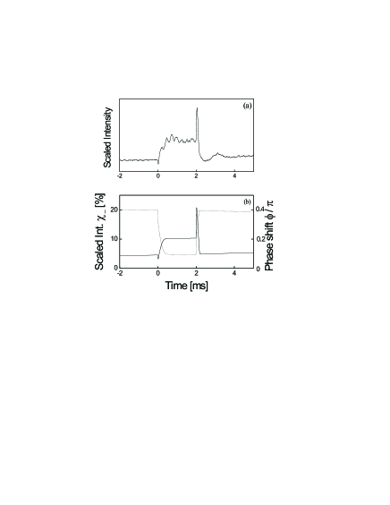
Figure 8: a) Observed intensity of the unlocked mode plotted versus time. During the time interval 0 ms$<$t$<2$ ms the total power coupled to the cavity is reduced by a factor of 2. b) shows a numerical simulation based on the adiabatic model. The intensity $\chi_{-}$ (solid line) and the corresponding phase $\phi$ (dotted line) are shown.

In the strong coupling regime our system shows an anomalous response to a change of the total intensity $I_{0}$ coupled to the cavity while keeping the same pumping asymmetry. This is shown in Fig. 8a) for $\chi_{0-}=45\%$. In this plot we have reduced $I_{0}$ by a factor two at $t=0$ ms and doubled it again at $t=2$ ms. As a first immediate reaction to the reduction $\chi_{-}$ rapidly drops on a time scale given by the cavity decay time ${\gamma_{c}}^{-1}$, as might be expected. However, this is counteracted by an approach of an increased steady state value on a slower time scale. When the old power level is reestablished, after a transient increase, $\chi_{-}$ drops back to nearly its original value. A numerical simulation based on our adiabatic model of Sec. III reproduces the experimental findings surprisingly well except the an unexplained additional ripple at about 3 kHz, which amounts to about six times the radial vibrational frequency. The calculations also show that during the drop of $I_{0}$ the phase shift of the unlocked mode with respect to the locked mode is reduced. Therefore the effective wavelength of the unlocked mode is shifted closer to resonance and the intensity increases.

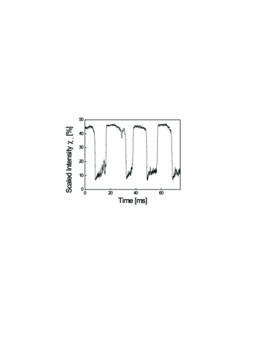
Figure 9: Bistable switching of $\chi_{-}$ during MOT loading for $\chi_{0-}=49\%$

The bistable character of the atom–cavity system can also be observed at work during MOT loading, yielding plots as that shown in Fig. 9, where $\chi_{-}$ switches between two steady state solutions ($\chi_{0-}=49\%$). Starting at t=0 at the high intensity level and hence with a deep lattice with comparably low atom number $N$, the MOT tends to increase $N$ until the interaction parameter exceeds the critical value and a jump occurs. Now the intensity is low and hence the lattice depth, while the temperature remains the same. This yields a decrease of the loading rate and thus a reduction of $N$ until the system jumps back to the previous state.

In order to control the performance of the locking the light reflected from the cavity originating from the locked travelling wave mode is monitored together with the light of the unlocked mode transmitted through one of the high reflectors . This allows to verify, that despite of the rapid changes in time observed for $\chi_{-}$ and $\phi$, the intra–cavity intensity of the counterpropagating locked mode remains well behaved. This is illustrated in Fig. 10 for $\chi_{0-}$=$45\%$. While in the lower trace rapid time evolution is observed the upper trace remains nicely constant. The residual structure seen in the upper trace is explained by imperfect separation of the contributions from the two modes due to limited quality of the polarization optics used.

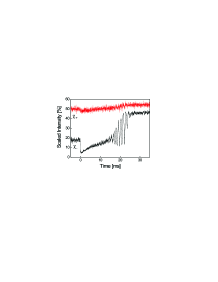
Figure 10: The intra–cavity intensities $\chi_{-}$ and $\chi_{+}$ of the unlocked mode (lower trace, recorded in transmission) and the locked mode (upper trace, obtained from the reflected light) are plotted versus time for $\chi_{0-}$=$45\%$.

VII Non–adiabatic Motion

The adiabatic model excellently explains the experimental findings regarding the intra–cavity intensity except for the pronounced oscillation feature observed in the $\chi_{0-}=43\%$–trace of Fig. 6. As has been discussed at the end of Sec. III the assumption of adiabaticity is not well justified for the radial degrees of the atomic motion. We came to the conclusion that for fast changes of the lattice well depth breathing oscillations should be excited which would produce corresponding oscillations in the intra–cavity intensity, if the system is operated near the frontier between the stable and the bistable regime, i.e., in the $43\%$ trace of Fig. 2. In fact this oscillation is observed in Fig. 6. An expanded version is shown in Fig. 12a).

As an experimental test of our interpretation in terms of radial breathing oscillations we have measured the momentum and position spread of the atomic ensemble in the radial direction during the observed intensity oscillations, finding the behavior shown in Fig. 11a). The black rectangles show the radial momentum spread of the atomic sample determined by time–of–flight measurements, while the open circles show the radial spread directly observed via in–situ images of the atoms in the lattice. The solid and dashed lines are trigonometric fits with $\pi$ phase delay, which confirm the expected anti–cyclic behavior. In Fig. 11b) we plot the frequency of the observed intensity oscillations versus the potential well depth confirming the expected square–root dependence.

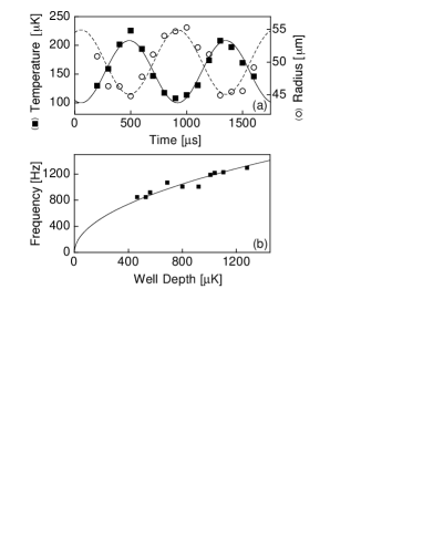
Figure 11: (a) Oscillation of the atomic position spread (circles) and momentum spread (rectangles). The solid and dashed lines are trigonometric fits with $\pi$ phase delay. (b) Oscillation frequency plotted versus the well depth. The solid line shows the expected square root dependence.

In order to include non–adiabatic aspects in our theoretical description we use the full set of 6N+2 equations of motion of Eq. (4) and Eq. (2) (i.e., 6N equations for the atomic positions and momenta and two equations for the amplitude and the phase of the unlocked intra–cavity mode). Since these equations are coupled and non–linear, the simulation of all $10^{6}$ atoms is beyond our computational capacities. Therefore, in our calculations we reduce the number of atoms to one hundred and work with an increased light shift per photon, such that the interaction strength acquires values which compare to the experiments. The artificially increased light shift per photon comes along with a correspondingly increased light shift acting on each atom. Hence, in order to maintain the potential well depth at the level used in the experiments, we work with correspondingly decreased incoupled intensities.

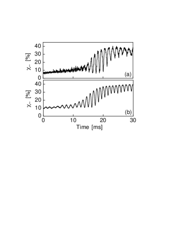
Figure 12: a) Experimental observation of radial breathing oscillations. (b) Simulation of the oscillations of (a) by means of solving the complete set of equations of motion for hundred atoms with an upscaled interaction strength.

The full model for one hundred atoms very accurately reproduces our calculations based on the adiabatic model shown in Fig. 7 except for the fact that in the vicinity of $\chi_{0-}\approx 43\%$ additional oscillations arise. This confirms once again that the assumption of adiabaticity of Sec. III is well justified for the axial degrees of freedom. We can quantitatively reproduce the frequency of the squeezing oscillation as is shown in Fig. 12 b). The experimental data are taken for $UN\approx 3.5$ and an axial vibrational frequency of 500 kHz, whereas for the theoretical curve $UN=2.0$ and 550 kHz was used. Applying the scaling factor 1.89 compensating for our systematic overestimation of the atom number similarly as in Sec. VI the measured interaction strength coincides with the theoretical value within $10\%$. The discrepancy in the vibrational frequencies lies within our observation uncertainty of ca. $10\%$. The non–adiabatic simulations of the system also reproduce the small frequency decrease in time observed in Fig. 12a).

VIII Conclusions

We conclude that optical lattices formed inside high finesse cavities open up an interesting new regime characterized by collective interactions significantly contributing to the atomic dynamics. This regime can be experimentally realized even far from an atomic resonance such that the interaction is entirely of dispersive nature. Although the combination of a high finesse with a large mode volume yields a small cavity resonance bandwidth, the experimental challenge of preventing intra–cavity intensity fluctuations can be handled. In the ring cavity studied here, specific parameter ranges are identified which allow to operate a stable lattice independent of the number of trapped atoms. Other regimes are found where dispersive optical bistability accompanied by self–induced breathing oscillations occur. The spatial phase of the lattice is not pinned by the phases of the incoupled laser beams, but rather determined by the strength of the atom–cavity interaction. The bistable behavior arises for asymmetric pumping and can be understood in terms of an adiabatic approximation for the atomic motion, whereas the general equations of motion must be considered to model the observed breathing oscillations. In this article we have only discussed selected aspects of the system dynamics. Other interesting phenomena could be studied, as for example collective atomic recoil lasing (CARL) Bon:94 , which has been recently observed for unidirectional pumping of the ring cavity Kru2:03 . The strong coupling regime might also be utilized for implementing novel laser cooling schemes, which rely on cavity–tailored coherent scattering, for example as described in Ref. Els:03 . Such schemes are highly desirable since they promise to extend laser cooling to new species and to operate in a density regime not yet accessible.

- (1) R. Grimm, M. Weidemüller and Y.B. Ovchinnikov, Adv. At., Mol., Opt. Phys. 42, 95 (2000).
- (2) D. Jaksch, C. Bruder, J. I. Cirac, C. W. Gardiner, and P. Zoller, Phys. Rev. Lett. 81, 3108 (1998).
- (3) T. Calarco, H.-J. Briegel, D. Jaksch, J. I. Cirac, and P. Zoller, J. Mod. Opt. 47, 2137 (2000).
- (4) B. Nagorny et al., Phys. Rev. A 67, 031401(R) (2003).
- (5) B. Nagorny, Th. Elsässer, A. Hemmerich, Phys. Rev. Lett., accepted for publication (2003).
- (6) D. Kruse et al., Phys. Rev. A 67, 051802(R) (2003).
- (7) D. Kruse, C. von Cube, C. Zimmermann, and Ph.W. Courteille, quant-ph/0305033 (2003).
- (8) A. Hemmerich, Phys. Rev. A. 60, 943 (1999).
- (9) A. C. Doherty, A. S. Parkins, S. M. Tan, and D. F. Walls, Phys. Rev. A. 56, 833 (1997).
- (10) P. Horak et al., Phys. Rev. Lett. 79, 4974 (1997).
- (11) G. Hechenblaikner, M. Gangl, P. Horak, and H. Ritsch, Phys. Rev. A. 58, 3030 (1998).
- (12) Th. Elsässer, B. Nagorny, and A. Hemmerich, Phys. Rev. A 67, 051401(R) (2003).
- (13) H.W. Chan, A.T. Black, and V. Vuletic, Phys. Rev. Lett. 90, 063003 (2003).
- (14) P.W.H. Pinkse, T. Fischer, P. Maunz, and G. Rempe, Nature 404, 365-368 (2000).
- (15) C. Hood et al., Science 287, 1457 (2000).
- (16) A. Lambrecht, E. Giacobino, and J.M. Courty, Opt. Commun. 115, 199 (1995).
- (17) J.A. Sauer et al., quant-ph/0309052 (2003).
- (18) M. Weidemüller, A. Görlitz, Th.W. Hänsch and A. Hemmerich, Phys. Rev. A. 58, 4647 (1998).
- (19) M. Gangl and H. Ritsch, Phys. Rev. A. 61, 043405 (2000).
- (20) A. Schoof, J. Grünert, S. Ritter, and A. Hemmerich, Opt. Lett. 26, 1562 (2001).
- (21) T. A. Savard, K. M. O’Hara, and J.E. Thomas, Phys. Rev. A. 56, R1095 (1997).
- (22) R. Bonifacio, L. De Salvo, L. M. Narducci, and E. J. D’Angelo, Phys. Rev. A 50, 1716 (1994)