Quantum state restoration by quantum cloning and measurement

Abstract

Copying information is an elementary operation in classical information processing. However, copying seems rather different in the quantum regime. Since the discovery of the universal quantum cloning machine, much has been found from the fundamental point of view about quantum copying. But a basic question as to the utility of universal quantum cloning remains. We have considered its application in quantum state restoration by using cloning circuit for state estimation. It might be expected that classical information from the state estimation might help restore the quantum state that was disturbed during storage in a quantum memory or transmission. We find that the fidelity of the final state is, interestingly, independent of error probabilities inside the memory/channel. However, this also turns out to impose a severe constraint on our original aims.

I Introduction

Quantum cloning has been studied intensively buzek96 ; gisin97 ; gisin98 ; werner98 and has played an important role in the development of the theory of quantum information. As copying information is one of the most fundamental processes in classical information processing, there has been some hope that quantum cloning may well be a useful operation in quantum information processing. However, only a few examples of its practical use have been discussed (See refs bechmann99 and galvao00 , for example).

We attempt first to utilize universal quantum cloning machine (UQCM) buzek96 ; buzek97 in restoring quantum states that are disturbed during quantum data storage in a quantum memory or transmission through a noisy quantum channel. Naturally, we have (approximate) quantum error-correction in mind as a further goal. By quantum cloning, we wish to reduce the redundancy which is necessary in both classical and quantum error-correcting schemes, because using many quantum channels might be expensive in resources. We have both quantum data storage and quantum communication in mind. However, we will use a communication-oriented view with Alice (sender) and Bob (receiver), which is common in the field of quantum information, in order to simplify the discussion. If we need to consider the data storage, we simply interpret Alice’s role as the writer of data and Bob’s role as the reader, who restores the quantum state for the subsequent processing.

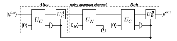
Our basic strategy is depicted in Fig. 1 and is as follows. By measuring two out of three qubits emerging from a quantum cloning circuit, Alice obtains some information about the initial state and sends this information to Bob using a classical channel. After transmitting the state through a noisy quantum channel, Bob also acquires information on the received state in the same fashion. If there is no energy dissipation during the transmission, Bob may be able to infer what kind of error has affected the state by comparing his measurement results with those of Alice. Then, he can apply the inverse of error operations to make the state as close as possible to the initial state.

One advantage of this idea is that it may work even if the error rates are very high. This is because Bob infers the type of error by measurement results, instead of through the error syndrome which relies on redundancy, so there is no need to assume low error probabilities, which are common in the standard error-correcting methods.

As well as utilizing the quantum cloning transformation, we also introduce an operation to reverse the effect of quantum measurement in order to improve the fidelity. Quantum measurements are, of course, irreversible, thus this reversal can be performed only approximately, when we wish this reversal to be a deterministic process.

We have found that the fidelity between initial and final states does not depend on the error probabilities during transmission. This can be seen as a consequence of the universality of the quantum cloning transformation. However, this feature imposes some constraint on the fidelity and our scheme exemplifies a situation in which use of both classical and quantum channels are not necessarily sufficient to improve the final fidelity.

This paper is organized as follows. In Section II, we describe how a quantum cloning circuit can be used to estimate quantum states. Then, in Section III, we explain the overall protocol. Section IV shows the approximate reversal of quantum measurement. Results and some discussions are given in Section V and concluding remarks in Section VI.

Figure 1: Quantum circuit representation of our state restoration protocol. Unitary transformation $U_{C}$ is a universal quantum cloning network with two extra qubits, which are represented by a single line in this figure. These extra qubits are observed after being processed with $U_{C}$ and the outcome is transmitted through a classical channel, which is a double line in the figure. Single qubit gates $U_{R}^{A}$ and $U_{R}^{B}$ are reversing operations and Bob’s error-correcting operation is included in $U_{R}^{B}$. These two operations are conditional on the outcome of the measurement. The effect of noise in the transmission channel is represented by a unitary transformation $U_{N}$ acting on both the state and its environment.

II State estimation by cloning

As in most literature on quantum error-correction steaneknill , here we take only bit and phase flips into account as the types of errors that may occur in the quantum channel. Thus, we wish to detect these two types of errors, whose occurrence may be described with two bit information, by comparing Alice’s and Bob’s measurement results. Since measurement on two qubits gives two bit classical information at most, it may be enough if the measurement can give the information on the tendency about the bit and the phase, i.e. one bit information for each. As we do not assume any a priori knowledge about the state, what we need to estimate is a quadrant of the space where the sate resides. Estimating the most probable quadrant for an incoming state by a UQCM circuit proceeds as follows. Let us consider Alice’s case, as Bob’s estimation is performed exactly the same way.

The initial state $|\psi^{\mathrm{in}}\rangle$ can be written as

$$|\psi^{\mathrm{in}}\rangle=\alpha|0\rangle+\beta e^{i\phi}|1\rangle,$$ (1)

where $\alpha,\beta\geq 0\>(\alpha^{2}+\beta^{2}=1)$ by neglecting the unimportant global phase. We consider only pure states as input for simplicity. The output state from Alice’s cloning transformation is

$$|\Psi_{A}^{\mathrm{cloned}}\rangle=\sqrt{\frac{2}{3}}(\alpha|000\rangle+\beta e^{i\phi}|111\rangle)+\sqrt{\frac{1}{6}}\left(\alpha(|011\rangle+|101\rangle)+\beta e^{i\phi}(|010\rangle+|100\rangle)\right).$$ (2)

Figure 2: Measurements on qubits from a cloning circuit. The second and the third qubits are measured using basis sets $\{|+\rangle,|0\rangle\}$ and $\{|0\rangle,|1\rangle\}$, respectively.

Figure 3: The probability distributions $p_{A}^{+0}$ and $p_{A}^{-1}$. It is easily seen that $p_{A}^{+0}$ is relatively higher where $\cos\phi>0$ and $\alpha^{2}>{\frac{1}{2}}$ and $p_{A}^{-1}$ has the opposite tendency. The other probability distribution, such as $p_{A}^{+1}$, is merely a combination of $\phi$-dependence of $p_{A}^{+0}$ and $\alpha^{2}$-dependence of $p_{A}^{-1}$.

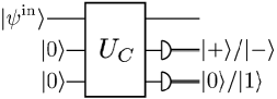
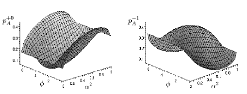
In order to obtain information on $\alpha,\beta$ and $\phi$, Alice performs projective measurements on the second and the third qubits in terms of basis sets {$|\pm\rangle=\frac{1}{\sqrt{2}}(|0\rangle\pm|1\rangle)$} and {$|0\rangle,|1\rangle$}, respectively, as shown in Fig. 2. The probability of having the outcome of $|+\rangle$ from the measurement on the second qubit of the state above is

$$p_{A(2)}^{+}={\frac{1}{2}}\left(1+\frac{4}{3}\alpha\beta\cos\phi\right),$$ (3)

where the subscript $A(2)$ stands for Alice’s second qubit, and the probability of having $|-\rangle$ is, thus, $p_{A(2)}^{-}={\frac{1}{2}}\left(1-\frac{4}{3}\alpha\beta\cos\phi\right)$. Since we are assuming that both $\alpha$ and $\beta$ are non-negative, if $p_{A(2)}^{+}>p_{A(2)}^{-}$ then $\cos\phi>0$ and if $p_{A(2)}^{+}<p_{A(2)}^{-}$ then $\cos\phi<0$. Therefore, by interpreting the outcome $|+\rangle$ (or $|-\rangle$) as a consequence of the relation between probabilities, $p_{A(2)}^{+}>p_{A(2)}^{-}$ (or $p_{A(2)}^{+}<p_{A(2)}^{-}$), Alice can estimate the range $\phi$ is in with a high probability.

Similarly, the probabilities of obtaining $|0\rangle$ and $|1\rangle$ from the measurement on the third qubit are $p_{A(3)}^{0}=\frac{1}{3}(1+\alpha^{2})$ and $p_{A(3)}^{1}=\frac{1}{3}(1+\beta^{2})$, respectively; hence we can say that the outcome $|0\rangle$ implies $\alpha>\beta$ and $|1\rangle$ implies the opposite. Fig. 3 shows a joint probability $p_{A}^{+0}$, which is the probability of outcomes + for the second qubit and 0 for the third qubit, and also $p_{A}^{-1}$ for comparison. Each probability distribution’s dependence on $\alpha^{2}$ and $\phi$ can be easily seen in this figure.

It is also worth noting for our protocol that the measurement described above does not change the tendency concerning $\alpha,\beta,$ and $\cos\phi$, as long as the implications are correct. For example, the state after Alice obtains + and 0 from her measurement can be written as

$$|\psi_{A}^{+0}\rangle = \frac{1}{||\cdot||}\left((\alpha+{\frac{1}{2}}\beta e^{i\phi})|0\rangle+{\frac{1}{2}}\beta e^{i\phi}|1\rangle\right)$$ (4)

$$= \frac{1}{||\cdot||}(\alpha^{\prime}|0\rangle+\beta^{\prime}e^{i\phi^{\prime}}|1\rangle),$$

where

$$\alpha^{\prime}=\left(\alpha^{2}+\alpha\beta\cos\phi+\frac{1}{4}\beta^{2}\right)^{\frac{1}{2}},\beta^{\prime}={\frac{1}{2}}\beta,$$

$$\phi^{\prime}=\phi-\tan^{-1}\frac{\beta\sin\phi}{2\alpha+\beta\cos\phi},$$ (5)

and the global phase is included in the normalization factor, which is denoted by $||\cdot||$ symbol. If the implications by the measurement are correct, i.e., $\alpha>\beta$ and $\cos\phi>0$, then $\alpha^{\prime},\beta^{\prime}$, and $\phi^{\prime}$ still satisfy the same relationship, $\alpha^{\prime}>\beta^{\prime}$ and $\cos\phi^{\prime}>0$.

III The protocol

Our task here is to send an unknown pure state $|\psi^{\mathrm{in}}\rangle$, a signal state, through a noisy channel with as high fidelity as possible. We take the ordinary input-output fidelity, which is defined by $F=\langle\psi^{\mathrm{in}}|\rho^{\mathrm{out}}|\psi^{\mathrm{in}}\rangle$ with a density matrix of the output state $\rho^{\mathrm{out}}$, as a figure of merit of the protocol’s performance. This means that our protocol is rather different from other quantum error-correcting schemes where we need to maintain the entanglement fidelity close to unity ent_fid .

Let us now describe the protocol in detail. In Fig. 1, $U_{C}$ is a quantum circuit implementing $1\rightarrow 2$ universal quantum cloning transformation. Since a $1\rightarrow 2$ UQCM requires one ancilla qubit to produce two output qubits, $U_{C}$ processes three qubits and outputs an entangled three-qubit state. In the figure, the second and third qubits are represented by a single line.

Alice lets the initial state $|\psi^{\mathrm{in}}\rangle$ go through a UQCM circuit and performs measurements on the second and third qubits emerging from the circuit to obtain some information on $|\psi^{\mathrm{in}}\rangle$. As these measurements, of course, disturb the signal state, Alice tries to make it as close to the initial state as possible. The reversal operation, $U_{R}^{A}$, should be performed deterministically depending on the outcome of the measurement, so it is a conditional unitary operation upon the outcome as a control bit. This is represented by a unitary gate connected with the classical information channel in Fig. 1. A filled black circle denotes a control bit. We will describe the details of the reversal operation later in Section IV. Alice also sends the results of her measurements to Bob through a classical communication channel, which we assume is error-free.

The effect of noise on the signal state during a transmission can be understood as a result of a unitary transformation $U_{N}$ acting on the state and its environment, which can be taken as a pure state $|0_{E}\rangle$, and the state of the environment after the transformation is discarded without being observed. This view leads to the standard Kraus representation of a quantum operation kraus , $\mathcal{E}(\rho)=\sum E_{i}\rho E_{i}^{\dagger}$. $E_{i}$ are operators acting on the state space of the principal system $\rho$ and they can be in general written as $E_{i}=\langle e_{i}|U|0_{E}\rangle$, where $|e_{i}\rangle$ are the orthonormal basis for the state space of the environment. If we denote the probability of a bit flip, which swaps $|0\rangle$ and $|1\rangle$, by $p_{bit}$ and that of a phase flip, which flips the sign of $|1\rangle$ while that of $|0\rangle$ is unchanged, is $p_{ph}$, the Kraus form of the error operation becomes

$$\mathcal{E}^{er}(\rho)=\sum_{i=0}^{4}E_{i}^{er}\rho{E_{i}^{er}}^{\dagger},$$ (6)

where $E_{0}^{er}=\sqrt{(1-p_{bit})(1-p_{ph})}I,E_{1}^{er}=\sqrt{p_{bit}(1-p_{ph})}\sigma_{x},E_{2}^{er}=\sqrt{p_{ph}(1-p_{bit})}\sigma_{z},$ and $E_{3}^{er}=\sqrt{p_{bit}p_{ph}}\sigma_{x}\sigma_{z}$.

Bob performs the same cloning transformation on the signal state he receives and measures the second and third qubits to acquire information on the state. Then, by comparing the outcome of his measurement with that from Alice, he infers what type of error has occurred during the transmission and carries out both the reversal and the error-correcting operations accordingly to output the final state $\rho^{\mathrm{out}}$. More specifically, if Alice’s and Bob’s outcomes from the measurement on the second qubit disagree, then Bob infers that there has been a phase flip and applies $\sigma_{x}$ to the state. Similarly, if their outcomes for the third qubit disagree, he flips the bit with $\sigma_{z}$. If both disagree, $\sigma_{x}\sigma_{z}$ will be applied.

IV The reversal of quantum measurement

Since a quantum state will be disturbed by any form of quantum measurement in principle, the signal state after the measurement for state estimation is no longer the same as the original state. However, in order to make the final fidelity as close as possible to unity, let us undertake an attempt to reverse the quantum measurement. Such a reversal, of course, can never be achieved perfectly, but probabilistic perfect reversals are possible and have been discussed in the context of quantum error-correction (ref_rev_op , for example). Nevertheless, what we discuss here is a (deterministic) approximate reversal, because the form of measurement, including the cloning transformation, is fixed in our case, thus, there is little freedom to apply the perfect reversal.

It is easily seen from Figs. 1 and 2 that measuring second and third qubits is equivalent to measuring the state of the environment, which is provided as a pure state $|0\rangle$ initially, after a unitary evolution $U_{C}$. Therefore, each of four measurement outcomes corresponds to an operation element in the Kraus representation of the quantum cloning transformation, $\mathcal{E}_{C}(|\psi\rangle\langle\psi|)=\sum_{i}E_{i}|\psi\rangle\langle\psi|{E_{i}}^{\dagger}$. Our analysis is similar in approach to the conditional dynamics utilized in quantum jump analyses of quantum trajectories martin98 . Operation elements can be expressed as

$$E_{0}=\frac{1}{2\sqrt{3}}\left(\begin{array}[]{cc}2&1\\ 0&1\end{array}\right), E_{1}=\frac{1}{2\sqrt{3}}\left(\begin{array}[]{cc}1&0\\ 1&2\end{array}\right),$$ (11)

$$E_{2}=\frac{1}{2\sqrt{3}}\left(\begin{array}[]{cc}2&-1\\ 0&1\end{array}\right), \mbox{and }E_{3}=\frac{1}{2\sqrt{3}}\left(\begin{array}[]{cc}-1&0\\ 1&-2\end{array}\right),$$ (16)

where subscripts $\{0,1,2,3\}$ denote measurement outcomes $\{+0,+1,-0,-1\}$. Hence, if we obtained a measurement outcome $i\in\{0,1,2,3\}$, the signal state after the measurement becomes

$$|\psi^{\prime}\rangle_{i}=\frac{E_{i}|\psi\rangle}{\sqrt{\langle\psi|E_{i}^{\dagger}E_{i}|\psi\rangle}}.$$ (17)

The approximate reversal of quantum measurement can be performed by the inverse of a unitary operator that is “similar” to the non-Hermitian operator, $E_{i}$. Thus, the question is simply to find a unitary matrix which is closest to a given matrix and is independent of the state $|\psi\rangle$, as we have no preferred input state. We can choose any metric for matrices to measure similarity between matrices. Here, we take a metric defined with the Hilbert-Schmidt norm, i.e., we define the distance between two matrices $A$ and $B$ as $\mathrm{dist}(A,B)=\left(\mathrm{Tr}[(A-B)^{\dagger}(A-B)]\right)^{1/2}$.

Suppose that we are approximating a square matrix $E$. By singular value decomposition bhatia , $E$ can be written as $E=VDW$, where $V$ and $W$ are certain unitary matrices and $D$ is a diagonal matrix with non-negative entries. Therefore, approximating $E$ by a unitary operation is now equivalent to approximating $D$ by a unitary. Such a unitary turns out to be the identity matrix, $I$, as follows. Let us denote a $2\times 2$ diagonal matrix $D$ by $\left(\begin{array}[]{cc}\mu&0\\ 0&\nu\end{array}\right)$. Without loss of generality, we can assume $\mu>\nu$, otherwise we can simply multiply $\sigma_{x}$ from both sides and include it in $V$ and $W$. In general, a $2\times 2$ unitary matrix can be expressed as $T=\left(\begin{array}[]{cc}a&b\\ -b^{*}&a^{*}\end{array}\right)$, with $|a|^{2}+|b|^{2}=1$, thus, the distance between these two matrices is given by

$$\mathrm{dist}(W,D)^{2} = \mathrm{Tr}[(T-\lambda D)^{\dagger}(T-\lambda D)]$$ (18)

$$= 2-\lambda((\mu+\nu)a+(\mu-\nu)a^{*})+\lambda^{2}\nu^{2},$$

with a certain positive normalization factor $\lambda$, corresponding to the denominator in Eq. (17). To minimize the value of Eq. (18), $a$ should be equal to 1 as both $\mu$ and $\nu$ are non-negative. It follows that the closest unitary matrix to a diagonal matrix with non-negative entries is the identity matrix and the closest unitary matrix to $E$ is $VW$. Since the singular value decomposition can be seen as a consequence of the polar decomposition, $VW$ is equal to the unitary matrix, $U$, that appears in the polar decomposition of $E$, $E=U\sqrt{E^{\dagger}E}$ bhatia2 . Reversal matrices for the operation elements in Eq. (11) are then written as

$${U_{R}^{0}}^{\dagger}=\frac{1}{\sqrt{10}}\left(\begin{array}[]{cc}3&-1\\ 1&3\end{array}\right), {U_{R}^{1}}^{\dagger}=\frac{1}{\sqrt{10}}\left(\begin{array}[]{cc}-3&-1\\ 1&-3\end{array}\right),$$ (23)

$${U_{R}^{2}}^{\dagger}=\frac{1}{\sqrt{10}}\left(\begin{array}[]{cc}3&1\\ -1&3\end{array}\right), \mbox{and }{U_{R}^{3}}^{\dagger}=\frac{1}{\sqrt{10}}\left(\begin{array}[]{cc}-3&1\\ -1&-3\end{array}\right).$$ (28)

Figure 4: Fidelity after applying the cloning and the reversal operations. Lower plane shows the “normal” fidelity of a $1\rightarrow 2$ UQCM, which is $5/6$.

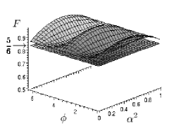
Fig. 4 shows the fidelity of the output state after applying the cloning transformation and the reversal operation. The plane at $F=\frac{5}{6}$ represents the normal fidelity of the output state from a $1\rightarrow 2$ UQCM. The effect of the reversal operation can be seen clearly in the figure: The fidelity is raised from $\frac{5}{6}$ by using the information form the measurement.

The reversal operation may change the quadrant in which the signal state lies in the $\alpha-\phi$ plane. In fact, it does change in some cases and thus measurement outcomes from Alice and Bob sometimes disagree even if there was no error and the estimation was perfect. However, as such a case is rather rare and the fidelity after the reversal is never lower than the case where we do not apply the reversal operation as in Fig. 4, we assume that the reversal operation does not affect the tendency about $\alpha,\beta$, and $\cos\phi$ so that the signal state stays in the same quadrant as long as the implications by the measurement are correct.

V Results

The numerically calculated fidelity between the initial and the final states is plotted in Fig. 5. The average fidelity over the $\alpha-\phi$ plane is 0.593, which is rather low if we regard the protocol as an error-correcting scheme. This value is even lower than that of a much simpler protocol, i.e., a direct measurement by Alice with a basis $\{|0\rangle,|1\rangle\}$ and the generation of either $|0\rangle$ or $|1\rangle$ by Bob according to Alice’s measurement result. This protocol gives an average fidelity of $\frac{2}{3}$ and it is optimal as state estimation massar95 . If our protocol is equivalent to state estimation, it is natural to have a fidelity lower than $\frac{2}{3}$. However, this is not the case, because estimating the state is different from the purpose of our protocol. All we wish to have is a high fidelity between the unknown initial state and the unknown final state. The fidelity can be higher than $\frac{2}{3}$ when the error rates of the channel is low enough and the measurements by Alice and Bob are weak enough.

Figure 5: The fidelity between the initial and the final states. The overall average is 0.593. The value of $F$ is always over $1/2$, except for two points, $(\alpha^{2},\phi)=(1/2,\pi/2)$ and $(1/2,3\pi/2)$.

Figure 6: Quantum circuit equivalent to that in Fig. 1 when the quantum channel is completely noisy. As the state Bob receives is completely random, it contains no information about the initial state $|\psi^{\mathrm{in}}\rangle$. Thus, the quantum channel is no longer necessary in such a case. The signal state is discarded after being processed by Alice’s $U_{C}$ and Bob follows the same procedure of the protocol after receiving a maximally mixed state, whose density matrix is given by $I/2$.

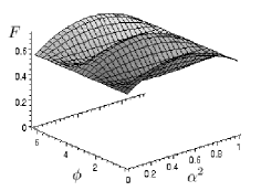
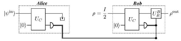
Nevertheless, the fidelity by our protocol is well below $\frac{2}{3}$. This is partly because of another interesting feature: The fidelity does not depend on the error rates, $p_{bit}$ and $p_{ph}$. That is, a perfect channel ($p_{bit}=p_{ph}=0$) and a completely noisy channel ($p_{bit}=p_{ph}=1/2$) give the same fidelity as in Fig. 5. This means that we can achieve the same value by providing a maximally mixed state to Bob without using the quantum channel. A quantum circuit equivalent to such an extreme situation is depicted in Fig. 6. Instead of a randomly disturbed signal state, a maximally mixed state, whose density matrix is given by $I/2$ with $I$ representing a $2\times 2$ identity matrix, is generated from a certain source and provided to Bob as a signal state. Bob performs the same procedure according to the protocol for the incoming completely mixed state. In this extreme case, components of our protocol are the same as those in the simple one whose fidelity reaches $\frac{2}{3}$, i.e., a measurement on an unknown quantum state, the transmission of the outcome through a classical channel, and the reproduction of state using the classical information. Therefore, the fidelity should be lower than $\frac{2}{3}$. The insensitivity of the fidelity to error rates means that it is always lower than $\frac{2}{3}$, regardless of the error rates.

We find it interesting that the completely noisy channel scenario (Fig. 6) gives the same fidelity as the case in which the quantum channel is completely noise-free, i.e., $U_{N}=I$ in Fig. 1. The information retained in the signal state does not have any effect on the fidelity in this protocol, as if all information that are immune to errors were absorbed by Alice’s measurement through the cloning transformation.

The reason for the fidelity’s insensitivity to error rates is in the symmetry among outputs of $U_{C}$, stemming from the universality of the transformation. In order to illustrate this, let $p_{\mathrm{ne}}^{01}$, for example, denote the probability that Bob obtains $1=\{+1\}$ by his measurement after Alice obtains $0=\{+0\}$ and there has been no error in the channel; the superscripts stand for Alice’s and Bob’s measurement results and the subscripts indicate the type of error occurred, ne=(no error), bf=(bit flip), pf=(phase flip) and bpf=(bit and phase flips). Similarly, let state vectors, such as $|\psi_{ne}^{01}\rangle$, denote final states in corresponding situations.

In our protocol, for example, $p_{\mathrm{ne}}^{00},p_{\mathrm{bf}}^{01},p_{\mathrm{pf}}^{02}$ and $p_{\mathrm{bpf}}^{03}$ are equal. Also, a set of final states, $|\psi_{\mathrm{ne}}^{00}\rangle,|\psi_{\mathrm{bf}}^{01}\rangle,|\psi_{\mathrm{pf}}^{02}\rangle$ and $|\psi_{\mathrm{bpf}}^{03}\rangle$ are the same as well. These can be verified straightforwardly by calculating each probability and state as

$$p_{\mathrm{ne}}^{00} = \langle\psi_{A}^{0}|E_{0}^{\dagger}E_{0}|\psi_{A}^{0}\rangle=\frac{1}{p_{A}^{0}}\langle\psi^{\mathrm{in}}|(E_{0}^{\dagger}E_{0})^{2}|\psi^{\mathrm{in}}\rangle,$$

$$p_{\mathrm{bf}}^{01} = \frac{1}{p_{A}^{0}}\langle\psi^{\mathrm{in}}|\sqrt{E_{0}^{\dagger}E_{0}}\sigma_{x}E_{1}^{\dagger}E_{1}\sigma_{x}\sqrt{E_{0}^{\dagger}E_{0}}|\psi^{\mathrm{in}}\rangle$$

$$= \frac{1}{p_{A}^{0}}\langle\psi^{\mathrm{in}}|(E_{0}^{\dagger}E_{0})^{2}|\psi^{\mathrm{in}}\rangle=p_{\mathrm{ne}}^{00},$$

$$p_{\mathrm{pf}}^{02} = \cdots=p_{\mathrm{ne}}^{00},$$

$$p_{\mathrm{bpf}}^{03} = \cdots=p_{\mathrm{ne}}^{00},$$

$$|\psi_{\mathrm{ne}}^{00}\rangle = \frac{E_{0}^{\dagger}E_{0}|\psi^{\mathrm{in}}\rangle}{\sqrt{\langle\psi^{\mathrm{in}}|(E_{0}^{\dagger}E_{0})^{2}|\psi^{\mathrm{in}}\rangle}}=\frac{E_{0}^{\dagger}E_{0}|\psi^{\mathrm{in}}\rangle}{\sqrt{p_{A}^{0}p_{\mathrm{ne}}^{00}}},$$

$$|\psi_{\mathrm{bf}}^{01}\rangle = \frac{1}{\sqrt{p_{A}^{0}p_{\mathrm{bf}}^{01}}}\sigma_{x}\sqrt{E_{1}^{\dagger}E_{1}}\sigma_{x}\sqrt{E_{0}^{\dagger}E_{0}}|\psi^{\mathrm{in}}\rangle,$$

$$= \frac{E_{0}^{\dagger}E_{0}|\psi^{\mathrm{in}}\rangle}{\sqrt{p_{A}^{0}p_{\mathrm{ne}}^{00}}}=|\psi_{\mathrm{ne}}^{00}\rangle,$$

$$|\psi_{\mathrm{pf}}^{02}\rangle = \cdots=|\psi_{\mathrm{ne}}^{00}\rangle,$$

$$|\psi_{\mathrm{bpf}}^{03}\rangle = \cdots=|\psi_{\mathrm{ne}}^{00}\rangle,$$ (29)

using specific forms of operation elements in Eq. (11). In Eqs. (V), $p_{A}^{0}$ denotes the probability for Alice to have the outcome $0=\{+0\}$ and $|\psi_{A}^{0}\rangle=\sqrt{E_{0}^{\dagger}E_{0}}|\psi^{\mathrm{in}}\rangle/\sqrt{p_{A}^{0}}$ is the state after Alice’s reversal operation.

As a result of the structure of the states and probabilities due to the symmetry in the quantum cloning transformation, many terms in the fidelity cancel out each other and all $p_{bit}$ and $p_{ph}$ disappear. For example, the fidelity after Alice measures $0=\{+0\}$ can be computed as $F^{0}=(1-p_{bit})(1-p_{ph})(p_{\mathrm{ne}}^{00}|\langle\psi^{\mathrm{in}}|\psi_{\mathrm{ne}}^{00}\rangle|^{2}+\cdots)+p_{bit}(1-p_{ph})(p_{\mathrm{bf}}^{01}|\langle\psi^{\mathrm{in}}|\psi_{\mathrm{bf}}^{01}\rangle|^{2}+\cdots)+p_{ph}(1-p_{bit})(p_{\mathrm{pf}}^{02}|\langle\psi^{\mathrm{in}}|\psi_{\mathrm{pf}}^{02}\rangle|^{2}+\cdots)+p_{bit}p_{ph}(p_{\mathrm{bpf}}^{03}|\langle\psi^{\mathrm{in}}|\psi_{\mathrm{bpf}}^{03}\rangle|^{2}+\cdots)=p_{\mathrm{ne}}^{00}|\langle\psi^{\mathrm{in}}|\psi_{\mathrm{ne}}^{00}\rangle|^{2}+\cdots$.

It is not hard to calculate the final fidelity analytically thanks to its independence on error rates. Assuming $I/2$ as the input state to Bob’s circuit, we obtain

$$F=\frac{1}{9}(5-2\alpha^{2}+2\alpha^{4})+\frac{8}{9}\alpha^{2}\beta^{2}\cos^{2}\phi,$$ (30)

which reproduces the same plot as Fig. (5). The average turns out to be $\frac{16}{27}=0.5926$, in accordance with our numerical result.

VI Concluding remarks

We investigated the possibility of the practical application of universal quantum cloning in quantum state restoration. We expected that the classical information from the state estimation by cloning would help improve the fidelity of the state after quantum data storage or transmission in a noisy environment. We have found that the fidelity does not depend on the error probabilities during transmission, thanks to the universality of the cloning transformation. However, this feature leads to a lower fidelity than its optimal value for state estimation of a single qubit, even if the initial state stays undisturbed when quantum memory/channel has low error rates. It implies that the acquisition of both classical and quantum information does not necessarily improve the fidelity even if nothing is discarded unnecessarily except for some information loss due to the interaction with the environment.

Although we have focused on the use of universal quantum cloning machine and individual measurement on two output qubits from it, there is a possibility of optimization of the cloning transformation and a joint measurement. Especially, if the number of possible input states $|\psi^{\mathrm{in}}\rangle$ is limited, we may be able to make use of the state-dependent quantum cloning bruss98 . A higher fidelity can be expected in such a case and it might be “useful” as an approximate error-correcting scheme in terms of real cost for implementation. We will discuss it elsewhere in the future.

References

- (1) V. Bužek and M. Hillery, Phys. Rev. A 54, 1844 (1996).
- (2) N. Gisin and S. Massar, Phys. Rev. Lett. 79, 2153 (1997).
- (3) N. Gisin, Phys. Lett. A 242, 1 (1998).
- (4) R. F. Werner, Phys. Rev. A 58, 1827 (1998).
- (5) H. Bechmann-Pasquinucci and N. Gisin, Phys. Rev. A 59, 4238 (1999).
- (6) E. F. Galvão and L. Hardy, Phys. Rev. A 62, 022301 (2000).
- (7) V. Bužek , S. L. Braunstein, M. Hillery, and D. Bruss, Phys. Rev. A 56, 3446 (1997).
- (8) For example, A. Steane, Proc. Roc. Soc. Lond. A 452, 2551 (1996); E. Knill and R. Laflamme, Phys. Rev. A 55, 900 (1997).
- (9) B. Schumacher, Phys. Rev. A 54, 2614 (1996); M. A. Nielsen, eprint quant-ph/9606012.
- (10) K. Kraus, States, Effects, and Operations (Springer-Verlag, Berlin, 1983).
- (11) M. A. Nielsen, C. M. Caves, B. Schumacher, and H. Barnum, Proc. R. Soc. Lond. A 454, 277 (1998); M. Koashi and M. Ueda, Phys. Rev. Lett. 82, 2598 (1999).
- (12) M. B. Plenio and P. L. Knight, Rev. Mod. Phys. 70, 101 (1998).
- (13) R. Bhatia, Matrix Analysis (Springer-Verlag, New York, 1997).
- (14) This is a simple proof of the problem for our purpose. A more formal proof of the same proposition can be found in bhatia .
- (15) S. Massar and S. Popescu, Phys. Rev. Lett. 74, 1259 (1995).
- (16) D. Bruß, D. P. DiVincenzo, A. Ekert, C. A. Fuchs, C. Macchiavello, and J. A. Smolin, Phys. Rev. A 57, 2368 (1998).