Optimized teleportation in Gaussian noisy channels

Abstract

We address continuous variable quantum teleportation in Gaussian quantum noisy channels, either thermal or squeezed-thermal. We first study the propagation of twin-beam and evaluate a threshold for its separability. We find that the threshold for purely thermal channels is always larger than for squeezed-thermal ones. On the other hand, we show that squeezing the channel improves teleportation of squeezed states and, in particular, we find the class of squeezed states that are better teleported in a given noisy channel. Finally, we find regimes where optimized teleportation of squeezed states improves amplitude-modulated communication in comparison with direct transmission.

1 Introduction

In a quantum channel, information is encoded in a set of quantum states, which are in general nonorthogonal and thus, even in principle, cannot be observed without disturbance. Therefore, their faithful transmission requires that the entire communication protocol is carried out by a physical apparatus that works without knowing or learning anything about the travelling signal. In this respect, quantum teleportation provides a remarkable mean for indirectly sending quantum states.

The key ingredient of quantum teleportation is an entangled bipartite state used to support the quantum communication channel [1]. This allows the preparation of an arbitrary quantum state at a distant place without directly transmitting it. In optical implementations of continuous variables quantum teleportation (CVQT), the entangled source is typically a twin-beam state of radiation (TWB), whose two modes are shared between the two parties. A faithful transmission of quantum information through the channel requires a large input-output fidelity, which in turn is an increasing function of the amount of entanglement. However, the propagation of a TWB in noisy channels unavoidably leads to degradation of entanglement, due to decoherence induced by losses and noise. Indeed, the effect of decoherence on TWB entanglement and, in turn, on teleportation fidelity, have been addressed by many authors [2, 3, 4, 5, 6, 7]. Thresholds for separablity of TWB have been established and teleportation of both classical and nonclassical states has been explicitly analyzed [8, 9]. In particular, in Ref. [9] it was investigated how much nonclassicality can be transferred by noisy teleportation in a zero temperature thermal bath. Moreover, the stability of squeezed states in a squeezed environment has been recently studied, showing that such nonclassical states loose their coherence faster than coherent states even if coupled with nonclassical reservoir [10]. The open question is then if there exist situations where squeezed states are favoured with respect to coherent ones, especially for quantum communication purporses.

In this paper we investigate the behavior of a TWB propagating through a Gaussian noisy channel, either thermal or squeezed-thermal, and address its performances for applications in quantum communication [11, 12]. As we will see, in presence of noise along the channel, teleportation of a suitable class of squeezed states can be an effective and robust protocol for amplitude-based communication compared to direct transmission.

Squeezed environments were addressed by many authors for preservation of the macroscopic quantum coherence. In fact, if squeezed quantum fluctuations are added to dissipation, a macroscopic superposition state preserves its coherence longer than in presence of dissipation alone [13]. Reference [14] showed that the interference fringes due to a superposition of two macroscopically distinct coherent states (“Schrödinger’s cat states”) could be improved by the inclusion of squeezed vacuum fluctuations. An interesting physical realization of an environment with squeezed quantum fluctuations based on quantum-non-demolition-feedback was proposed in reference [15]. Effective squeezed-bath interactions were studied in references [16, 17], where the technique of quantum-reservoir engineering [18] was actually used to couple a pair of two-state atoms to an effective squeezed reservoir.

The paper is structured as follows: in sections 2 and 3 we describe the evolution of a TWB in a squeezed-thermal bath and study its separability by means of the partial transposition criterion; section 4 addresses the TWB coupled with the non classical environment as a resource for quantum teleportation of squeezed states; in section 5 we compare the performances of direct transmission and teleportation. In section 6 we draw some concluding remarks.

2 Twin beam coupled with a squeezed thermal bath

The propagation of a TWB interacting with a squeezed-thermal bath can be modelled as the coupling of each part of the state with a non-zero temperature squeezed reservoir. The dynamics can be described by the two-mode Master equation [19]

$$\frac{d\rho_{t}}{dt} = \{\Gamma(1+N)L[a]+\Gamma(1+N)L[b]+\Gamma NL[a^{{\dagger}}]+\Gamma NL[b^{{\dagger}}]$$ (1)

$$\hskip 28.45274pt+\Gamma M\mathcal{M}[a^{{\dagger}}]+\Gamma M^{*}\mathcal{M}[a]+\Gamma M\mathcal{M}[b^{{\dagger}}]+\Gamma M^{*}\mathcal{M}[b]\}\rho_{t}\,,\;$$

where $\rho_{t}\equiv\rho(t)$ is the system’s density matrix at the time $t$, $\Gamma$ is the damping rate, $N$ and $M$ are the effective photons number and the squeezing parameter of the bath respectively, $L[O]$ is the Lindblad superoperator, $L[O]\rho_{t}=O\rho_{t}O^{{\dagger}}-\frac{1}{2}O^{{\dagger}}O\rho_{t}-\frac{1}{2}\rho_{t}O^{{\dagger}}O$, and $\mathcal{M}[O]\rho_{t}=O\rho_{t}O-\frac{1}{2}OO\rho_{t}-\frac{1}{2}\rho_{t}OO$. The terms proportional to $L[a]$ and $L[b]$ describe the losses, whereas the terms proportional to $L[a^{{\dagger}}]$ and $L[b^{{\dagger}}]$ describe a linear phase-insensitive amplification process. Of course, the dynamics of the two modes are independent on each other.

Thanks to the differential representation of the superoperators in equation (1), the corresponding Fokker-Planck equation for the two-mode Wigner function $W\equiv W(x_{1},y_{1};x_{2},y_{2})$ is

$$\partial_{t}W = \frac{\Gamma}{2}\sum_{j=1}^{2}\>\left(\partial_{x_{j}}x_{j}+\partial_{y_{j}}y_{j}\right)W+\frac{\Gamma}{2}\sum_{j=1}^{2}\>\left\{\frac{1}{2}\Re{\rm e}[M]\left(\partial^{2}_{x_{j}x_{j}}-\partial^{2}_{y_{j}y_{j}}\right)\right.$$ (2)

$$\quad+\left.\Im{\rm m}[M]\>\partial^{2}_{x_{j}y_{j}}+\frac{1}{2}\left(N+\frac{1}{2}\right)\left(\partial^{2}_{x_{j}x_{j}}+\partial^{2}_{y_{j}y_{j}}\right)\right\}W\;,$$

which, introducing $\tau=\Gamma t/\gamma$ and $\gamma=(2N+1)^{-1}$, reduces to the standard form

$$\partial_{\tau}W=\left\{-\sum_{j=1}^{4}\partial_{x_{j}}\>a_{j}(\underline{x})+\frac{1}{2}\sum_{i,j=1}^{4}\partial^{2}_{x_{i}x_{j}}\>d_{ij}\right\}W\,,$$ (3)

where, for sake of simplicity, we put $\underline{x}=(x_{1},y_{1};x_{2},y_{2})\equiv(x_{1},x_{2};x_{3},x_{4})$. In equation (3) $a_{j}(\underline{x})$ and $d_{ij}$ are the matrix elements of the drift and diffusion matrices $\mathbf{A}(\underline{x})$ and $\mathbf{D}$ respectively, which are given by

$$\mathbf{A}(\underline{x})=-\frac{\gamma}{2}\,\underline{x}\,,$$ (4)

$$\mathbf{D}=\left(\begin{array}[]{cccc}\frac{1}{4}+\frac{\gamma}{2}\,\Re{\rm e}[M]&\gamma\,\Im{\rm m}[M]&0&0\\ \gamma\,\Im{\rm m}[M]&\frac{1}{4}-\frac{\gamma}{2}\,\Re{\rm e}[M]&0&0\\ 0&0&\frac{1}{4}+\frac{\gamma}{2}\,\Re{\rm e}[M]&\gamma\,\Im{\rm m}[M]\\ 0&0&\gamma\,\Im{\rm m}[M]&\frac{1}{4}-\frac{\gamma}{2}\,\Re{\rm e}[M]\end{array}\right)\,.$$ (9)

Notice that in our case the drift term is linear in $\underline{x}$ and the diffusion matrix does not depend on $\underline{x}$. We assume $M$ as real and a TWB as starting state i.e. $\rho_{0}\equiv\rho_{\rm TWB}=|{\rm TWB}\rangle\rangle\langle\langle{\rm TWB}|$, where $|{\rm TWB}\rangle\rangle=\sqrt{1-x^{2}}\sum_{p}\>x^{a^{{\dagger}}a}\>|p\rangle|p\rangle$. The TWB corresponds to the Wigner function

$$W_{0}(x_{1},y_{1};x_{2},y_{2})=\frac{\exp\left\{\displaystyle{-\frac{(x_{1}+x_{2})^{2}}{4\sigma_{+}^{2}}-\frac{(y_{1}+y_{2})^{2}}{4\sigma_{-}^{2}}-\frac{(x_{1}-x_{2})^{2}}{4\sigma_{-}^{2}}-\frac{(y_{1}-y_{2})^{2}}{4\sigma_{+}^{2}}}\right\}}{(2\pi)^{2}\>\sigma_{+}^{2}\sigma_{-}^{2}}$$ (10)

with $\sigma_{\pm}^{2}=\frac{1}{4}e^{\pm 2\lambda}$ and $\lambda$, $x=\tanh\lambda$, being the squeezing parameter of the TWB. Now the solution of the Fokker-Planck (3) is given by [19]

$$W_{\tau}(x_{1},y_{1},x_{2},y_{2})=\frac{\exp\left\{\displaystyle{-\frac{(x_{1}+x_{2})^{2}}{4\Sigma_{1}^{2}}-\frac{(y_{1}+y_{2})^{2}}{4\Sigma_{2}^{2}}-\frac{(x_{1}-x_{2})^{2}}{4\Sigma_{3}^{2}}-\frac{(y_{1}-y_{2})^{2}}{4\Sigma_{4}^{2}}}\right\}}{(2\pi)^{2}\>\Sigma_{1}\>\Sigma_{2}\>\Sigma_{3}\>\Sigma_{4}}$$ (11)

where $\Sigma_{j}^{2}=\Sigma_{j}^{2}(\lambda,\Gamma,n_{\rm th},n_{\rm s})$, $j=1,2,3,4$, are

$$\begin{array}[]{lll}\Sigma_{1}^{2}=\sigma_{+}^{2}e^{-\Gamma t}+D_{+}^{2}(t)\,,&&\Sigma_{2}^{2}=\sigma_{-}^{2}e^{-\Gamma t}+D_{-}^{2}(t)\,,\\ \mbox{}\\ \Sigma_{3}^{2}=\sigma_{-}^{2}e^{-\Gamma t}+D_{+}^{2}(t)\,,&&\Sigma_{4}^{2}=\sigma_{+}^{2}e^{-\Gamma t}+D_{-}^{2}(t)\,,\end{array}$$ (12)

and

$$D_{\pm}^{2}(t)=\frac{1+2N\pm 2M}{4}\left(1-e^{-\Gamma t}\right)$$ (13)

with $\left|M\right|\leq(2N+1)/2$. The latter condition is already enforced by the positivity condition for the Fokker-Planck’s diffusion coefficient, which requires

$$M\leq\sqrt{N(N+1)}\,.$$ (14)

If we assume the environment as composed by a set of oscillators excited in a squeezed-thermal state of the form $\nu=S(r)\rho_{\rm th}S^{\dagger}(r)$, with $S(r)=\exp\{\frac{1}{2}r[a^{{\dagger}2}-a^{2}]\}$ and $\rho_{\rm th}=(1+n_{\rm th})^{-1}[n_{\rm th}/(1+n_{\rm th})]^{a^{\dagger}a}$, then we can rewrite the parameters $N$ and $M$ in terms of the squeezing and thermal number of photons $n_{\rm s}=\sinh^{2}r$ and $n_{\rm th}$ respectively. Then we get [10]

$$M = \left(1+2\,n_{\rm th}\right)\sqrt{n_{\rm s}(1+n_{\rm s})}\,,$$ (15)

$$N = n_{\rm th}+n_{\rm s}(1+2\,n_{\rm th})\>.$$ (16)

Using this parametrization, the condition (14) is automatically satisfied.

3 Separability

A quantum state of a bipartite system is separable if its density operator can be written as $\varrho=\sum_{k}p_{k}\sigma_{k}\otimes\tau_{k}$, where $\{p_{k}\}$ is a probability distribution and $\tau$’s and $\sigma$’s are single-system density matrices. If a state is separable the correlations between the two systems are of purely classical origin. A quantum state which is not separable contains quantum correlations i.e. it is entangled. A necessary condition for separability is the positivity of the density matrix $\varrho^{T}$, obtained by partial transposition of the original density matrix (PPT condition) [20]. In general PPT has been proved to be only a necessary condition for separability; however, for some specific sets of states, PPT is also a sufficient condition. These include states of $2\times 2$ and $2\times 3$ dimensional Hilbert spaces [21] and Gaussian states (states with a Gaussian Wigner function) of a bipartite continuous variable system, e.g. the states of a two-mode radiation field [22, 23]. Our analysis is based on these results. In fact, the Wigner function of a twin-beam produced by a parametric source is Gaussian and the evolution inside active fibers preserves such character. Therefore, we are able to characterize the entanglement at any time and find conditions on the fiber’s parameters to preserve it after a given fiber length. The density matrix’s PPT property can be rephrased as a condition on the covariance matrix of the two modes Wigner function $W(x_{1},y_{1};x_{2},y_{2})$. We have that a state is separable iff

$$\mathbf{V}+\frac{i}{4}\mathbf{\Omega}\geq 0$$ (17)

where

$$\begin{array}[]{cc}\mathbf{\Omega}=\left(\begin{array}[]{cc}\mathbf{J}&\mathbf{0}\\ \mathbf{0}&\mathbf{J}\end{array}\right)&\mbox{and}\quad\mathbf{J}=\left(\begin{array}[]{cc}0&1\\ -1&0\end{array}\right)\,.\end{array}$$ (23)

and

$$V_{pk}=\langle\Delta\xi_{p}\>\Delta\xi_{k}\rangle=\int\!\!{\rm d}^{4}\xi\>\>\Delta\xi_{p}\>\Delta\xi_{k}\>W(\xi)\,,$$ (24)

with $\Delta\xi_{j}=\xi_{j}-\langle\xi_{j}\rangle$, and $\underline{\xi}=\{x_{1},y_{1},x_{2},y_{2}\}$. The explicit expression of the covariance matrix associated to the Wigner function (11) is

$$\mathbf{V}=\frac{1}{2}\left(\begin{array}[]{cccc}\Sigma_{1}^{2}+\Sigma_{3}^{2}&0&\Sigma_{1}^{2}-\Sigma_{3}^{2}&0\\ 0&\Sigma_{2}^{2}+\Sigma_{4}^{2}&0&\Sigma_{2}^{2}-\Sigma_{4}^{2}\\ \Sigma_{1}^{2}-\Sigma_{3}^{2}&0&\Sigma_{1}^{2}+\Sigma_{3}^{2}&0\\ 0&\Sigma_{2}^{2}-\Sigma_{4}^{2}&0&\Sigma_{2}^{2}+\Sigma_{4}^{2}\end{array}\right)\,,$$ (29)

and, then, condition (17) is satisfied when

$$\Sigma_{1}^{2}\>\Sigma_{4}^{2}\geq\frac{1}{16}\,,\quad\quad\Sigma_{2}^{2}\>\Sigma_{3}^{2}\geq\frac{1}{16}\,.$$ (30)

Notice that changing the sign of $M$ leaves conditions (30) unaltered.

By solving these inequalities with respect to time, $t$ we find that the two-mode state becomes separable for $t>t_{\rm s}$, where the threshold time $t_{\rm s}=t_{\rm s}(\lambda,\Gamma,n_{\rm th},n_{\rm s})$ is given by

$$t_{\rm s}=\frac{1}{\Gamma}\log\left(f+\frac{1}{1+2n_{\rm th}}\sqrt{f^{2}+\frac{n_{\rm s}(1+n_{\rm s})}{n_{\rm th}(1+n_{\rm th})}}\right)\,,$$ (31)

and we defined

$$f\equiv f(\lambda,n_{\rm th},n_{\rm s})=\frac{(1+2\,n_{\rm th})\>\left[1+2\,n_{\rm th}-e^{-2\,\lambda}(1+2\,n_{\rm s})\right]}{4\,n_{\rm th}(1+n_{\rm th})}\,.$$ (32)

As one may expect, $t_{\rm s}$ decreases as $n_{\rm th}$ and $n_{\rm s}$ increase. Moreover, in the limit $n_{\rm\rm s}\rightarrow 0$, the threshold time (31) reduces to the case of a non squeezed bath, in formula [4, 7]

$$t_{0} = t_{\rm s}(\lambda,\Gamma,n_{\rm th},0)$$ (33)

$$= \frac{1}{\Gamma}\log\left(1+\frac{1-e^{-2\,\lambda}}{2\,n_{\rm th}}\right)\,.$$

In order to see the effect of a squeezed bath on the entanglement time we define the function

$$G(\lambda,n_{\rm th},n_{\rm s}) \equiv \frac{t_{\rm s}-t_{\rm 0}}{t_{0}}\,.$$ (34)

In this way, when $G>0$, the squeezed bath gives a threshold time longer than the one obtained with $n_{\rm s}=0$, shorter otherwise. These results are illustrated in figure 1, where we plot equation (34) as a function of $n_{\rm s}$ for different values of $n_{\rm th}$ and $\lambda$. Since $G$ is always negative, we conclude that coupling a TWB with a squeezed-thermal bath destroys the correlations between the two channels faster than the coupling with a non squeezed environment.

4 Optimized quantum teleportation

In this section we study continuous variable quantum teleportation (CVQT) assisted by a TWB propagating through a squeezed-thermal environment. Let us remind the CVQT protocol: the sender and the receiver, say Alice and Bob, share a two-mode state described by the density matrix $\rho_{12}$, where the subscripts refer to modes 1 and 2 respectively: mode 1 is sent to Alice, the other to Bob. The goal of CVQT is teleporting an unknown state $\sigma$, corresponding to the mode 3, from Alice to Bob. In order to implement the teleportation, Alice first performs a heterodyne detection on modes 3 and 1, i.e. she jointly measures a couple of two-mode quadratures. The POVM of the measurement is given by

$$\Pi_{13}(z)=\frac{1}{\pi}\>D_{1}(z)|\mathbb{I}\rangle\rangle_{13}{}_{31}\langle\langle\mathbb{I}|D_{1}^{{\dagger}}(z)\,,\;$$ (35)

where $|\mathbb{I}\rangle\rangle_{13}\equiv\sum_{v}\>|v\rangle_{1}|v\rangle_{3}$, and $D_{1}(z)\equiv\exp\{za^{{\dagger}}-z^{*}a\}$ is the displacement operator acting on mode 1. Each measurement outcome is a complex number $z$, which is sent to Bob via a classical communication channel, and used by him to apply a displacement $D(z)$ to mode 2 such to obtain the quantum state $\rho_{\rm tele}$ which, in an ideal case, coincides with the input signal $\sigma$ [24, 25]. The Wigner function of the heterodyne POVM is given by [26]

$$W[\Pi_{13}(z)](x_{1},y_{1};x_{3},y_{3})=\frac{1}{\pi^{2}}\>\delta\big{(}(x_{1}-x_{3})+x\big{)}\>\delta\big{(}(y_{1}+y_{3})-y\big{)}\,,\;$$ (36)

with $z=x+iy$, and since, using Wigner functions, the trace between two operators can be written as [27]

$${\rm Tr}\>[O_{1}\>O_{2}]=\pi\>\int\!\!d^{2}w\>W[O_{1}](w)\>W[O_{2}](w)\,,$$ (37)

the heterodyne probability distribution is given by [28]

$$p(z) = \pi^{3}\int\!\!\!\!\int\!\!dx_{1}\,dy_{1}\int\!\!\!\!\int\!\!dx_{2}\,dy_{2}\int\!\!\!\!\int\!\!dx_{3}\,dy_{3}\>W[\sigma](x_{3},y_{3})\>$$ (38)

$$\hskip 28.45274pt\times W[\rho_{12}](x_{1},y_{1};x_{2},y_{2})\>$$

$$\hskip 42.67912pt\times W[\Pi_{13}(z)](x_{1},y_{1};x_{3},y_{3})\,W[\mathbb{I}_{2}](x_{2},y_{2})\,,\;$$

while the conditional state of mode 2 is

$$W[\rho_{2}(z)](x_{2},y_{2}) = \frac{\pi^{2}}{p(z)}\>\int\!\!\!\!\int\!\!dx_{1}\,dy_{1}\int\!\!\!\!\int\!\!dx_{3}\,dy_{3}\>W[\sigma](x_{3},y_{3})\>$$ (39)

$$\hskip 28.45274pt\times W[\rho_{12}](x_{1},y_{1};x_{2},y_{2})\>$$

$$\hskip 42.67912pt\times W[\Pi_{13}(z)](x_{1},y_{1};x_{3},y_{3})\,W[\mathbb{I}_{2}](x_{2},y_{2})\,,$$

where $W[\mathbb{I}_{2}](x_{2},y_{2})=\pi^{-1}$. Thanks to equation (36) and after the integration with respect to $x_{3}$ and $y_{3}$, we have

$$W[\rho_{2}(z)](x_{2},y_{2}) = \frac{1}{\pi\,p(z)}\>\int\!\!\!\!\int\!\!dx_{1}\,dy_{1}\>W[\sigma](x_{1}+x,-y_{1}+y)\>$$ (40)

$$\hskip 56.9055pt\times W[\rho_{12}](x_{1},y_{1};x_{2},y_{2})$$

$$= \frac{1}{\pi\,p(z)}\>\int\!\!\!\!\int\!\!dx_{1}\,dy_{1}\>W[\sigma](x_{1},y_{1})\>$$

$$\hskip 56.9055pt\times W[\rho_{12}](x_{1}-x,-y_{1}+y;x_{2},y_{2})\,.$$

Now we perform the displacement $D(z)$ on mode 2. Since

$$W[D(z)\>\rho\>D^{{\dagger}}(z)](x_{j},y_{j})=W[\rho](x_{j}-x,y_{j}-y)\,,$$

we obtain

$$W[\rho^{\prime}_{2}(z)](x_{2},y_{2}) = \frac{1}{\pi\,p(z)}\>\int\!\!\!\!\int\!\!dx_{1}\,dy_{1}\>W[\sigma](x_{1},y_{1})\>$$ (41)

$$\hskip 28.45274pt\times W[\rho_{12}](x_{1}-x,-y_{1}+y;x_{2}-x,y_{2}-y)\,.$$

with $\rho^{\prime}_{2}(z)\equiv D(z)\>\rho_{2}(z)\>D^{{\dagger}}(z)$. The output state of CVQT is obtained integrating equation (41) with respect to all the possible outcomes of heterodyne detection

$$W[\rho_{\rm tele}](x_{2},y_{2})=\int\!\!d^{2}z\>p(z)\>W[\rho^{\prime}_{2}(z)](x_{2},y_{2})\,.$$ (42)

Finally, when the shared state is the one given in equation (11), equation (42) rewrites as follows

$$W[\rho_{\rm tele}](x_{2},y_{2}) = \int\!\!\!\!\int\!\!\frac{dx^{\prime}\>dy^{\prime}}{4\pi\>\Sigma_{2}\>\Sigma_{3}}\>$$ (44)

$$\hskip 14.22636pt\times\exp\left\{-\frac{(x^{\prime}-x_{2})^{2}}{4\Sigma_{3}^{2}}-\frac{(y^{\prime}-y_{2})^{2}}{4\Sigma_{2}^{2}}\right\}\>W[\sigma](x^{\prime},y^{\prime})$$

$$= \int\!\!\frac{d^{2}w}{4\pi\>\Sigma_{2}\>\Sigma_{3}}\>\exp\left\{-\frac{(\Re{\rm e}[w])^{2}}{4\Sigma_{3}^{2}}-\frac{(\Im{\rm m}[w])^{2}}{4\Sigma_{2}^{2}}\right\}\>$$

$$\hskip 14.22636pt\times W[D(w)\>\sigma\>D^{{\dagger}}(w)](x_{2},y_{2})\,,$$

which shows that the map $\mathcal{L}$, describing CVQT assisted by a TWB propagating through a squeezed-thermal environment, is given by

$$\rho_{\rm tele} \equiv \mathcal{L}\sigma$$ (45)

$$= \int\!\!\frac{d^{2}w}{4\pi\>\Sigma_{2}\>\Sigma_{3}}\>\exp\left\{-\frac{(\Re{\rm e}[w])^{2}}{4\Sigma_{3}^{2}}-\frac{(\Im{\rm m}[w])^{2}}{4\Sigma_{2}^{2}}\right\}\>$$

$$\hskip 14.22636pt\times D(w)\>\sigma\>D^{{\dagger}}(w)\,,\;$$

i.e. the teleportation protocol corresponds to a generalized Gaussian noise. Notice that if $n_{\rm s}\rightarrow 0$, from equations (12), (15) and (16) one has

$$\Sigma_{2}^{2},\Sigma_{3}^{2}\rightarrow\sigma_{-}^{2}\>e^{-\Gamma t}+\frac{1+2n_{\rm th}}{4}(1-e^{-\Gamma t})\,,$$ (46)

which is the noise due to a thermalized quantum channel [8]. The map (45) can be extended to the case of a general Gaussian noise as follows

$$\mathcal{L}_{\rm gen}\sigma=\int\!\!\frac{d^{2}w}{\pi\>\sqrt{{\rm det}[\mathbf{C}]}}\>\exp\left\{-\underline{w}\>\mathbf{C}\>\underline{w}^{T}\right\}\>D(w)\>\sigma\>D^{{\dagger}}(w)\,,\;$$ (47)

where $\underline{w}$ is the row vector $\underline{w}=(\Re{\rm e}[w],\Im{\rm m}[w])$ and $\mathbf{C}$ is the covariance matrix of the noise [2].

Now, in order to use CVQT as a resource for quantum information processing, we look for a class of squeezed states which achieves an average teleportation fidelity greater than the one obtained teleporting coherent states in the same conditions. The Wigner function of the squeezed state $\sigma=|\alpha,\zeta\rangle\langle\alpha,\zeta|$, $|\alpha,\zeta\rangle=D(\alpha)S(\zeta)|0\rangle$, is given by (we assume the squeezing parameter $\zeta$ as real)

$$W[\sigma](x_{3},y_{3})=\frac{2}{\pi}\>\exp\Bigg{\{}-\frac{2\>(x_{3}-a)^{2}}{e^{-2\zeta}}-\frac{2\>(y_{3}-b)^{2}}{e^{2\zeta}}\Bigg{\}}\;,$$ (48)

with $a=\Re{\rm e}[\alpha]$, $b=\Im{\rm m}[\alpha]$. Thanks to equations (44) and (48), we have

$$W[\rho_{\rm tele}](x,y)=\frac{2\>\exp\left\{\displaystyle{-\frac{2\>(x-a)^{2}}{e^{-2\zeta}+8\>\Sigma_{3}^{2}}-\frac{2\>(y-b)^{2}}{e^{2\zeta}+8\>\Sigma_{2}^{2}}}\right\}}{\pi\sqrt{(e^{2\zeta}+8\>\Sigma_{2}^{2})(e^{-2\zeta}+8\>\Sigma_{3}^{2})}}\>\;,$$ (49)

where we suppressed all the subscripts. The average teleportation fidelity is thus given by

$$\overline{F}_{\zeta,{\rm tele}}(\lambda,\Gamma,n_{\rm th},n_{\rm s}) \equiv \pi\int\!\!\!\!\int\!\!{\rm d}x\>{\rm d}y\>W[\sigma](x,y)\>W[\rho_{\rm out}](x,y)$$ (50)

$$= \Big{(}\sqrt{(e^{2\zeta}+4\>\Sigma_{2}^{2})(e^{-2\zeta}+4\>\Sigma_{3}^{2})}\Big{)}^{-1}\,,$$

which attains its maximum when

$$\zeta=\zeta_{\rm max}\equiv\frac{1}{2}\log\left(\frac{\Sigma_{2}}{\Sigma_{3}}\right)\,,$$ (51)

and, after this maximization, reads as follows

$$\overline{F}_{\rm tele}(\lambda,\Gamma,n_{\rm th},n_{\rm s})=\frac{1}{1+4\>\Sigma_{2}\>\Sigma_{3}}\,.$$ (52)

For $n_{\rm s}\rightarrow 0$ we have $\Sigma_{2}=\Sigma_{3}$, and thus then $\zeta_{\rm max}\rightarrow 0$, i.e. the input state that maximizes the average fidelity (50) reduces to a coherent state. In other words, in a non squeezed environment the teleportation of coherent states is more effective than that of squeezed states. Moreover, equation (52) shows that meanwhile the TWB becomes separable, i.e. $\Sigma_{2}^{2}\>\Sigma_{3}^{2}\geq\frac{1}{16}$ (see equations (30)), one has $\overline{F}_{\rm tele}\leq 0.5$. We remember that when the average fidelity is less than 0.5, the same results can be achieved using classical (non entangled) shared states [24, 29]: in our case, it could be possible to verify the separability of the shared state simply studying the fidelity achieved teleporting squeezed states. Notice that the classical limit $\overline{F}_{\rm tele}=0.5$, which was derived in the case of coherent state teleportation [29], still holds when we wish to teleport a squeezed state with a fixed squeezing parameter. Finally, the asymptotic value of $\overline{F}_{\rm tele}$ for $\Gamma t\rightarrow\infty$ is

$$\overline{F}_{\rm tele}^{(\infty)}=\frac{1}{2\>(1+n_{\rm th})}\,,$$ (53)

which does not depend on the number of squeezed photons and is equal to $0.5$ only if $n_{\rm th}=0$. This last result is equivalent to say that in presence of a zero-temperature enviroment, no matter if it is squeezed or not, the TWB is non-separable at every time.

In figure 2 we plot $\overline{F}_{\rm tele}$ as a function of $\Gamma t$ for different values of $\lambda$, $n_{\rm th}$ and $n_{\rm s}$. As $n_{\rm s}$ increases, the non classicity of the thermal bath starts to affect the teleportation fidelity and we observe that the best results are obtained when the state to be teleported is the squeezed state that maximizes (50). Furthermore the difference between the two fidelities increases as $n_{\rm s}$ increases. Notice that there is an interval of values for $\Gamma t$ such that the coherent state teleportation fidelity is less than the classical limit $0.5$, although the shared state is still entangled.

5 Teleportation vs direct transmission

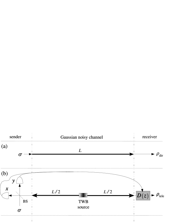
Figure 3: Direct and teleportation-assisted transmission. (a) In direct transmission, the sender directly sends state $\sigma$ through the Gaussian noisy channel: the state arriving at the receiver is $\rho_{\rm dir}$. (b) In teleportation-assisted transmission, the sender mixes at the balanced beam splitter BS the state $\sigma$ to be transmitted with one of the two mode of the shared state, arriving from the Gaussian noisy channel, and then he measures the quadrature $x$ and $y$, respectively, of the output modes. This result is classically communicated to the receiver, which applies a displacement $D(z)$, $z=x+iy$, to the output state, obtaining $\rho_{\rm tele}$ (see section 4 for details). Notice that the length of the direct transmission line is twice the effective length of the teleportation-assisted transmission one.

This section is devoted to investigate whether the results obtained in the previous sections can be used to improve quantum communication using non classical states. We suppose to have a communication protocol where information is encoded onto the field amplitude of a set of squeezed states of the form $|\alpha,\zeta\rangle$ with fixed squeezing parameter. In figure 3 we show a schematic diagram for direct and teleportation-assisted communication. As one can see from the figure, direct transmission line’s length $L$ is twice the effective length of the teleportation-assisted scheme: this is due to the fact that the two modes of the shared state are chosen to be propagating in opposite directions.

When we directly send the squeezed state (48) through a squeezed noisy quantum channel, the state arriving at the receiver is

$$W[\rho_{\rm dir}](x,y)=\frac{2\>\exp\left\{\displaystyle{-\frac{2\>(x-a\>e^{-\Gamma t^{\prime}/2})^{2}}{e^{-2\zeta-\Gamma t^{\prime}}+4D_{+}^{2}}-\frac{2\>(y-b\>e^{-\Gamma t^{\prime}/2})^{2}}{e^{2\zeta-\Gamma t^{\prime}}+4D_{-}^{2}}}\right\}}{\pi\sqrt{(e^{-2\zeta-\Gamma t^{\prime}}+4D_{+}^{2})(e^{2\zeta-\Gamma t^{\prime}}+4D_{-}^{2})}}\>\;,$$ (54)

with $D_{\pm}^{2}$, evaluated at time $t^{\prime}$, given in equation (13) and time $t^{\prime}$ is twice the time $t$ implicitly appearing in equation (49), because of the previously explained choice. Equation (54) is the Wigner function of the state $\rho_{\rm dir}$, solution of the single-mode Master equation

$$\frac{{d}\rho_{t}}{{d}t}=\{\Gamma(1+N)L[a]+\Gamma NL[a^{{\dagger}}]+\Gamma M\mathcal{M}[a^{{\dagger}}]+\Gamma M^{*}\mathcal{M}[a]\}\rho_{t}\,,\;$$ (55)

where $\Gamma$, $N$, $M$ and the superoperators $L[O]$ and $\mathcal{M}[O]$ have the same meaning as in equation (1). As in case of quantum teleportation, we can define the direct transmission fidelity (see equation (50)), obtaining

$$F_{\zeta,\alpha,{\rm dir}}(\Gamma,n_{\rm th},n_{\rm s})=\frac{\exp\left\{\displaystyle{-\frac{a^{2}(1-e^{-\Gamma t^{\prime}/2})^{2}}{2\>\Sigma_{a}^{2}(t^{\prime})}-\frac{b^{2}(1+e^{-\Gamma t^{\prime}/2})^{2}(t^{\prime})}{2\>\Sigma_{b}^{2}(t^{\prime})}}\right\}}{2\sqrt{\Sigma_{a}^{2}(t^{\prime})\>\Sigma_{b}^{2}(t^{\prime})}}\>\;.$$ (56)

where

$$\Sigma_{a}^{2}(t^{\prime}) = \mbox{$\frac{1}{4}$}e^{-2\zeta}(1+e^{-\Gamma t^{\prime}})+D_{+}^{2}(t^{\prime})\;,$$ (57)

$$\Sigma_{b}^{2}(t^{\prime}) = \mbox{$\frac{1}{4}$}e^{2\zeta}(1+e^{-\Gamma t^{\prime}})+D_{-}^{2}(t^{\prime})\,.$$ (58)

Since $F_{\zeta,\alpha,{\rm dir}}$ depends on the amplitude $\alpha=a+ib$ of the state to be transmitted, in order to evaluate the average fidelity here we assume that the trasmitter sends squeezed states with fixed squeezed parameter and with amplitudes distributed according to the Gaussian

$$\mathcal{P}(\alpha)=\frac{1}{2\pi\Delta^{2}}\exp\Bigg{\{}-\frac{|\alpha|^{2}}{2\Delta^{2}}\Bigg{\}}\,.$$ (59)

The average direct transmission fidelity reads as follows

$$\overline{F}_{\zeta,{\rm dir}} = \int\!\!d^{2}\alpha\>\mathcal{P}(\alpha)\>F_{\zeta,\alpha,{\rm dir}}(\Gamma,n_{\rm th},n_{\rm s})$$ (60)

$$= \frac{1}{2}\Bigg{\{}\sqrt{\big{[}(1-e^{-\Gamma t^{\prime}/2})\Delta^{2}+\Sigma_{a}^{2}(t^{\prime})\big{]}\big{[}(1-e^{-\Gamma t^{\prime}/2})\Delta^{2}+\Sigma_{b}^{2}(t^{\prime})\big{]}}\Bigg{\}}^{-1}\;,$$ (61)

which, for $\Gamma t\rightarrow\infty$ and using equation (51), reduces to

$$\overline{F}_{{\rm dir}}^{(\infty)}=\frac{1}{2}\Big{(}\sqrt{g_{+}(n_{\rm th},n_{\rm s})\>g_{-}(n_{\rm th},n_{\rm s})}\Big{)}^{-1}\,,$$ (62)

with

$$g_{\pm}(n_{\rm th},n_{\rm s}) = \frac{1}{4}\Bigg{[}1+\sqrt{1+8\>n_{\rm s}(1+n_{\rm s})\pm 4\>(1+2\>n_{\rm s})\sqrt{n_{\rm s}(1+n_{\rm s})}}$$

$$\hskip 14.22636pt+2\Big{(}n_{\rm s}+n_{\rm th}+2\>n_{\rm s}n_{\rm th}\pm(1+2\>n_{\rm th})\sqrt{n_{\rm s}(1+n_{\rm s})}\Big{)}\Bigg{]}+\Delta^{2}\,.$$

Teleportation is a good resource for quantum communication in noisy channel when $\overline{F}_{\zeta,{\rm tele}}\geq\overline{F}_{\zeta,{\rm dir}}$, which gives a threshold $\Delta_{\rm th}^{2}$ on the width $\Delta^{2}$ of the distribution (59)

$$\Delta_{\rm th}^{2}(\lambda,\Gamma,n_{\rm th},n_{\rm s}) = \frac{1}{2\>(1-e^{-\Gamma t})^{2}}\bigg{\{}-\big{[}\Sigma_{a}^{2}(2t)+\Sigma_{b}^{2}(2t)\big{]}$$ (63)

$$\hskip 14.22636pt+\sqrt{\big{[}\Sigma_{a}^{2}(2t)-\Sigma_{b}^{2}(2t)\big{]}^{2}+\big{(}\overline{F}_{\zeta,{\rm tele}}\big{)}^{-2}}\bigg{\}}\;,$$

where $\overline{F}_{\zeta,{\rm tele}}$ of Eq. (50) is evaluated at time $t$ and, then, $t^{\prime}=2t$.

In figure 4 we plot $\overline{F}_{\zeta,{\rm tele}}$ and $\overline{F}_{\zeta,{\rm dir}}$ with $\zeta=\zeta_{\rm max}$ for different values of the other parameters. We see that teleportation is an effective and robust resource for communication as the channel becomes more noisy and $\Delta^{2}$ larger. Moreover, when $n_{\rm th},n_{\rm s}\rightarrow 0$, one obtains the following finite value for the threshold

$$\Delta_{\rm th}^{2}(\lambda,\Gamma,0,0)=\frac{e^{\Gamma t}-1+e^{-2\lambda}}{2\>e^{-\Gamma t}(1-e^{-\Gamma t})^{2}}\,,$$ (64)

i.e. teleportation assisted communication can be more effective than direct transmission even for pure dissipation at zero temperature.

6 Conclusions

In this work we have studied the propagation of a TWB through a Gaussian quantum noisy channel, either thermal or squeezed-thermal, and have evaluated the threshold time after which the state becomes separable. Moreover, we have explicitly found the completely positive map for the teleportated state using the Wigner formalism.

We have found that the threshold for a squeezed environment is always shorter than for a purely thermal one. On the other hand, we have shown that squeezing the channel is a useful resource when entanglement is used for teleportation of squeezed states. In particular, we have found the class of squeezed states which optimize teleportation fidelity. The squeezing parameter of such states depends on the channel parameters themselves. In these conditions, the teleportation fidelity is always larger than the one achieved by teleporting coherent states. Moreover, there are no regions of useless entanglement, i.e. the fidelity approaches the classical limit $\overline{F}=0.5$ when the TWB becomes separable.

Finally, we have found regimes where the optimized teleportation of squeezed states can be used to improve the transmission of amplitude-modulated signals through a squeezed-thermal noisy channel. The transmission performances have been investigated by means of input-output fidelity, comparing the direct transmission with the teleportation one. Actually, decoherence mechanisms are different between these two channels: in the teleportation channel the fidelity is reduced due to the interaction of the TWB with the squeezed-thermal bath; in direct transmission the signal is directly coupled with the non-classical environment and, then, fidelity is affected by the degradation of the signal itself. The performance of CVQT as a quantum communication channel in nonclassical environment obviously depends on the parameters of the channel itself, but our analysis has shown that if the signal is drawn from the class of squeezed states that optimize teleportation fidelity, and the probability distribution of the transmitted state amplitudes is wide enough, then teleportation is more effective and robust as the environment becomes more noisy.

Figure 1: Plots of the ratio $G=(t_{\rm s}-t_{0})/t_{0}$ as a function of the number of squeezed photons $n_{\rm s}$ for different values of the TWB parameter $\lambda$ and of the number of thermal photons $n_{\rm th}$. The values of $n_{\rm th}$ are chosen to be: (a) $n_{\rm th}=10^{-6}$, (b) $10^{-3}$, (c) $10^{-1}$ and (d) $1$, while the solid lines, from bottom to top, refer to $\lambda$ varying between 0.1 to 1.0 with steps of 0.15.

Figure 2: Plots of the average teleportation fidelity. The solid and the dashed lines represent squeezed and coherent state fidelity, respectively, for different values of the number of squeezed photons $n_{\rm s}$: (a) $n_{\rm s}=0$, (b) $0.1$, (c) $0.3$, (d) $0.7$. In all the plots we put the TWB parameter $\lambda=1.5$ and number of thermal photons $n_{\rm th}=0.5$. The dot-dashed vertical line indicates the threshold $\Gamma t_{\rm s}$ for the separability of the shared state: when $\Gamma t>\Gamma t_{\rm s}$ the state is no more entangled. Notice that, in the case of squeezed state teleportation, the threshold for the separability corresponds to $\overline{F}=0.5$.

Figure 4: Plots of average teleportation (equation (50)) and direct communication (equation (61)) fidelity as functions of $\Gamma t$ for different values of $n_{\rm th}$ and $n_{\rm s}$: (a) $n_{\rm th}=n_{\rm s}=0$; (b) $n_{\rm th}=0.3$ and $n_{\rm s}=0$; (c) $n_{\rm th}=0.5$ and $n_{\rm s}=0$: (d) $n_{\rm th}=0.5$ and $n_{\rm s}=0.3$. In all the plots the solid line referes to $\overline{F}_{\rm tele}$ with $\lambda=1.5$, whereas the dashed lines are $\overline{F}_{\rm dir}$ with (from top to bottom) $\Delta^{2}=0.1,0.5,1,5$. The squeezing parameter is chosen to be $\zeta=\zeta_{\rm max}$, which maximizes teleportation fidelity. Notice that direct transmission fidelity is evaluated in a time $t$ equal twice the time of teleportation (see the scheme in figure 3). The dot-dashed vertical line indicates the threshold $\Gamma t_{\rm s}$ for the separability of the shared state used in teleportation.

References

• [1] C. H. Bennett et al., Phys. Rev. Lett 70, 1895 (1993).
• [2] D. Wilson, J. Lee and M. S. Kim, quant-ph/0206197 v3 (2002).
• [3] J. Lee, M. S. Kim and H. Jeong, Phys. Rev A 62, 032305 (2000).
• [4] J. S. Prauzner-Bechcicki, quant-ph/0211114 v2 (2003).
• [5] A. Vukics, J. Janszky and T. Kobayashi, Phys. Rev. A 66, 023809 (2002).
• [6] W. P. Bowen et al., Phys. Rev. A 67, 032302 (2003).
• [7] M. G. A Paris, Entangled light and applications in Progress in Quantum Physics Research, V. Krasnoholovets Ed., Nova Publisher, in press.
• [8] M. Ban, M. Sasaki and M. Takeoka, J. Phys. A: Math. Gen. 35, L401 (2002).
• [9] M. Takeoka, M. Ban and M. Sasaki, J. Opt. B: Quantum Semiclass. Opt. 4, 114 (2002).
• [10] K. S. Grewal, Phys Rev A 67, 022107 (2003).
• [11] M. A. Nielsen and I. L. Chuang, Quantum Computation and Quantum Information (Cambridge University Press, Cambridge, 2000).
• [12] S. Olivares and M. G. A. Paris, Binary optical communication in single-mode and entangled quantum noisy channels, preprint quant-ph/0309096
• [13] T. A. B. Kennedy and D. F. Walls, Phys. Rev. A 37, 152 (1988).
• [14] W. J. Munro and M. D. Reid, Phys. Rev. A 52, 2388 (1995).
• [15] P. Tombesi and D. Vitali, Phys. Rev. A 50, 4253 (1994).
• [16] S. G. Clark and A. S. Parkins, Phys. Rev. Lett. 90, 047905 (2003).
• [17] S. G. Clark, A. Peng, M. Gu and S. Parkins, quant-ph/0307064.
• [18] N. Lütkenhaus, J. I. Cirac and P. Zoller, Phys. Rev. A 57, 548 (1998).
• [19] D. F. Walls and G. J. Milburn, Quantum Optics (Springer-Verlag, Berlin, 1994).
• [20] A. Peres, Phys. Rev. Lett. 77, 1413-1415 (1996).
• [21] P. Horodecki, M. Lewenstein, G. Vidal and I. Cirac, Phys. Rev. A 62, 032310 (2000).
• [22] Lu-Ming Duan, G. Giedke, J. I. Cirac and P. Zoller, Phys. Rev. Lett. 84 2722 (2000).
• [23] R. Simon, Phys. Rev. Lett. 84 2726 (2000).
• [24] S. L. Braunstein and H. J. Kimble, Phys. Rev. Lett. 80, 869 (1998).
• [25] A. Furusawa et. al., Science 282, 706 (1998).
• [26] M. G. A. Paris, M. Cola and R. Bonifacio, J. Opt. B 5, S360 (2003).
• [27] K. Cahill and R. Glauber, Phys. Rev. 177, 1857 (1969).
• [28] S. Olivares, M. G. A. Paris and R. Bonifacio, Phys. Rev. A 67, 032314 (2003).
• [29] S. L. Braunstein, C. A. Fuchs and H. J. Kimble, J. Mod. Opt. 47, 267 (2000).
Refer to caption