Binary optical communication in single-mode and entangled quantum noisy channels

Abstract

We address binary optical communication in single-mode and entangled quantum noisy channels. For single-mode we present a systematic comparison between direct photodetection and homodyne detection in realistic conditions, i.e. taking into account the noise that occurs both during the propagation and the detection of the signals. We then consider entangled channels based on twin-beam state of radiation, and show that with realistic heterodyne detection the error probability at fixed channel energy is reduced in comparison to the single-mode cases for a large range of values of quantum efficiency and noise parameters.

1 Introduction

Classical information may be conveyed to a receiver through quantum channels. To this aim a transmitter prepares a quantum state drawn from a collection of known states and sends it through a given quantum channel. The receiver retrieves the information by measuring the channel, such to discriminate among the set of possible preparations, and to determine the transmitted signal. The encoding states are generally not orthogonal and also when orthogonal signals are transmitted, they usually lose orthogonality because of noisy propagation through the communication channel. Therefore, in general, no measurement allows the receiver to distinguish perfectly between the signals [1, 2] and the need of optimizing the detection strategy unavoidably arises.

In binary communication based on optical signals, information is encoded into two quantum states of light. Amplitude modulation-keyed signals (AMK), consist in two states of a single-mode radiation field, which are given by $\varrho_{j}=|\psi_{j}\rangle\langle\psi_{j}|$, $j=1,2$, with $|\psi_{1}\rangle=|\psi_{0}\rangle$ and $|\psi_{2}\rangle=D(\alpha)|\psi_{0}\rangle$, where $|\psi_{0}\rangle$ is a given seed state, usually taken as the vacuum, $D(\alpha)=\exp(\alpha a^{\dagger}-\alpha^{*}a)$ denotes the displacement operator, and the complex amplitude $\alpha$ may be taken as real without loss of generality. The reason to choose AMK signals lies in the fact that displacing a state is a simple operation, which is experimentally achievable by a linear coupler and strong reference beam [3]. Another binary encoding, based on displacement, is given by phase shift-keyed signals (PSK) $|\psi_{1}\rangle=D(-\alpha)|\psi_{0}\rangle$ and $|\psi_{2}\rangle=D(\alpha)|\psi_{0}\rangle$. In the following, we will refer to the AMK situation only, though all the results hold also for PSK. The price to pay for such a convenient encoding stage is that, for any choice of the seed state, the two signals are always not orthogonal, and thus a nonzero probability of error appears in their discrimination [4]. If we consider equal a priori probabilities for the two signals, the optimal quantum measurement to discriminate them with minimum error probability is the projection-valued measure $\{M_{j}\}_{j=1,2}$, $M_{1}+M_{2}=\mathbb{I}$, corresponding to [1]

$$M_{j}=\sum_{k}T[(-)^{j}\lambda_{k}]|\lambda_{k}\rangle\langle\lambda_{k}|\,,\;$$ (1)

where $|\lambda_{k}\rangle$ is an eigenstate of the hermitian operator $\Lambda=\rho_{2}-\rho_{1}$ with eigenvalue $\lambda_{k}$, and $T[x]$ is the unit step function, which is zero for negative $x$, one for positive and $T(0)=\frac{1}{2}$. The probability of inferring the symbol $j$ when $i$ is transmitted is given by $P(j|i)=\hbox{Tr}\{\varrho_{i}\>M_{j}\}$, $j,i=1,2$, such that the average error probability in binary communication is given by $P_{{\rm e}}=\frac{1}{2}\left\{P(1|2)+P(2|1)\right\}$. The minimum of $P_{\rm e}$, corresponding to the optimal measurement (1), reads as follows

$$P_{{\rm e}}=\frac{1}{2}\left(1-\sqrt{1-|\langle\psi_{2}|\psi_{1}\rangle|^{2}}\right)\,,$$ (2)

and is known as the Helstrom bound [2]. In particular, for a pair of AMK signals we have

$$P_{{\rm e}}=\frac{1-\sqrt{1-\exp(-2N)}}{2}\,,$$ (3)

where with $N$ we denote the average number of photons in the channel per use, i.e. $N=\frac{1}{2}{\rm Tr}[a^{{\dagger}}a(\rho_{0}+\rho_{\alpha})]=\frac{1}{2}|\alpha|^{2}+n_{0}$, where $n_{0}=\langle\psi_{0}|a^{\dagger}a|\psi_{0}\rangle$ is the average photon number of the seed state. For the sake of brevity, we will refer to $N$ also as to the energy of the channel. Notice that for a pair of PSK signals the same bound in equation (3) holds; however, the expression for $N$ is now given by $N=|\alpha|^{2}+n_{0}$.

Binary communication has been the subject of much attention, mostly concerning the design and the implementation of optimal quantum detection processes, to distinguish nonorthogonal signals with reduced error probability, possibly approaching the Helstrom bound given in equation (2). The relevant parameter in this optimization is the energy of the channel, which itself limits the communication rate of the channel. After the pioneering work of Helstrom [1], a near-optimum receiver for AMK signals based on direct detection was proposed in [5], whereas an optimum receiver approaching the minimum error probability (3) (based on photon counting and feedback) has been suggested in [6]. More recently, various efforts has been made to find out optimum detection operators and decision processes for more general signals and in presence of noise [7, 8, 9, 10]. Indeed, when one has at disposal a given set of quantum signals, the problem becomes that of finding the optimal receivers [5, 6] and detection schemes [11, 12] and to compare their performances with those of realistic detectors. Following this way, some studies were made on the effects of thermal noise on the optimum detection for a coherent AMK channel [13].

In this paper we focus our attention on protocols for binary communications where both AMK signals and receivers can be realized with current technology. As we will see, the various sources of loss and noise can be described as an overall Gaussian noise. Our analysis allows to unravel the different contributions and to compare receivers in realistic working regimes. The purpose is twofold: on one hand we perform a systematic comparison between direct and homodyne detection in presence of noise during the propagation and the detection stages, in order to find in which working regimes a receiver should be preferred. On the other hand, we show that binary communication can be improved by using achievable sources of entanglement and realistic heterodyne receivers. Indeed, it has been recently shown that in ideal conditions (perfect detection and noiseless propagation) entanglement improves the performances of a binary channel, i.e. it reduces the error probability in the discrimination of the symbols [14, 15]. Motivated by these results, we investigate the error probability of entangled channels in realistic conditions, taking into account the unavoidably noise that occurs during the propagation and the detection. Since we are interested in assessing entanglement as an effective resource, we compare entangled channels with the corresponding realistic single-mode channels.

The paper is structured as follows. In Section 2 we address single-mode channels that uses direct or homodyne detection as receivers, and compare the corresponding error probabilities both in ideal and realistic situations, i.e. in presence of noise. In section 3 we describe a binary communication scheme based on entangled twin-beam state of radiation that employs multiport homodyne or heterodyne detection in the measurements stage. As we will see, there are regimes where the error probability is less than in a single mode channel, also when the noise affects propagation and detection. Finally, in section 4 we summarize our results giving some concluding remarks.

2 Single Mode Communication

2.1 Direct detection - Ideal case

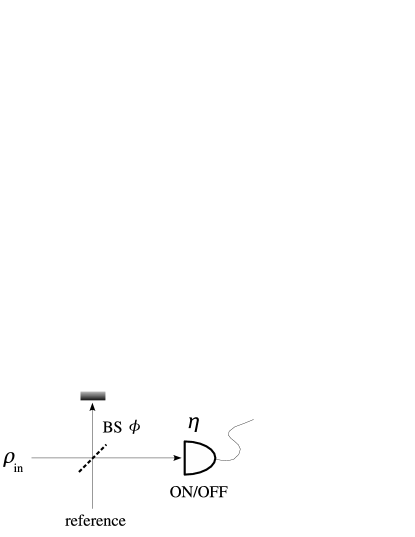
Figure 1: Scheme of the receiver based on direct detection. The signal to be processed is mixed at a beam splitter of transmissivity $\tau=\cos^{2}\phi$ with a given coherent reference state. Then, at the output, one of the two modes is ignored or absorbed, whereas the other one is revealed by on/off photodetection. In the ideal case $\rho_{\rm in}=\rho_{\mu}=|\mu\rangle\langle\mu|$, $\mu=0,\alpha$, and the the detection efficiency is $\eta=1$. In presence of noise, $\rho_{\rm in}$ is given by equation (18) and $\eta<1$.

A scheme based on direct detection, to discriminate the set $\{|0\rangle,|\alpha\rangle\}$, can be implemented as in figure 1 [5]. It consists of a beam splitter (BS), in which the state to be processed, either $|0\rangle$ or $|\alpha\rangle$, is mixed with a given coherent reference state, say $|\beta\rangle$. The outgoing mode is subsequently revealed by on/off photodetection, i.e. by a detector which checks the presence or absence or any number of photons.

The operator describing the action of a BS on the modes $a$ and $b$ of the field is

$$U_{\phi}=\exp\left\{\phi(a^{{\dagger}}b-ab^{{\dagger}})\right\}\;,\qquad\phi=\arctan\sqrt{\frac{1-\tau}{\tau}}\;,$$ (4)

where $\tau=\cos^{2}\phi$ is the BS transmissivity and $a$, $a^{{\dagger}}$ and $b$, $b^{{\dagger}}$ are the annihilation and creation operators for the two modes, respectively. If the input state is $|\alpha\rangle_{a}|\beta\rangle_{b}\equiv|\alpha\rangle_{a}\otimes|\beta\rangle_{b}$, $|\alpha\rangle_{a}$ and $|\beta\rangle_{b}$ being coherent states, the output state is given by $|\alpha\rangle_{a}|\beta\rangle_{b}\longrightarrow|\alpha\cos\phi+\beta\sin\phi\rangle_{a}\,|-\alpha\sin\phi+\beta\cos\phi\rangle_{b}$. By choosing the amplitude of the reference as $\beta=-\alpha/\tan\phi$, we obtain, at the output, the vacuum when the input state is $|\alpha\rangle$, and $|-\alpha\cos\phi\rangle$ for vacuum input, in formula

$$|\alpha\rangle\rightsquigarrow|0\rangle\qquad\mbox{and}\qquad|0\rangle\rightsquigarrow|-\alpha\cos\phi\rangle.$$ (5)

In order to discriminate the two input signals, one performs a simple on/off photodetection: when the output is the vacuum the detector doesn’t click, otherwise it clicks. This measurement is described by the probability operator-valued measure (POVM) $\{\Pi_{0},\Pi_{1}\}$, where $\Pi_{0}=|0\rangle\langle 0|$ and $\Pi_{0}+\Pi_{1}=\mathbb{I}$, i.e. we assumed unit detector efficiency. The error probability, $K_{{\rm e}}$, is defined as:

$$K_{{\rm e}}=\frac{1}{2}\{K(0|\alpha)+K(\alpha|0)\}\,,$$ (6)

where $K(0|\alpha)$ and $K(\alpha|0)$ are the probabilities of inferring that the input state is $|0\rangle$ when it is actually $|\alpha\rangle$ and vice versa. In our case

$$K(0|\alpha) = \Tr\{U_{\phi}\,\rho_{\alpha}\otimes\rho_{\beta}\,U_{\phi}^{{\dagger}}\,\Pi_{1}\otimes\mathbb{I}\}\,,$$ (7)

$$K(\alpha|0) = \Tr\{U_{\phi}\,\rho_{0}\otimes\rho_{\beta}\,U_{\phi}^{{\dagger}}\,\Pi_{0}\otimes\mathbb{I}\}\,,$$ (8)

where $\rho_{\mu}=|\mu\rangle\langle\mu|$, $\mu=0,\alpha,\beta$. We obtain

$$K(0|\alpha) = |\langle 0|\Pi_{1}|0\rangle|^{2}=0$$ (9)

$$K(\alpha|0) = |\langle-\alpha\cos\phi|\Pi_{0}|-\alpha\cos\phi\rangle|^{2}=\exp\{-|\alpha|^{2}\cos^{2}\phi\},$$ (10)

such that Eq. (6) rewrites as

$$K_{{\rm e}}=\frac{\exp(-|\alpha|^{2}\cos^{2}\phi)}{2}=\frac{\exp(-2N\cos^{2}\phi)}{2}.$$ (11)

with $N=\Tr\{a^{{\dagger}}a\,(\rho_{0}+\rho_{\alpha})\}=\frac{1}{2}|\alpha|^{2}$. Notice that in the limit $|\alpha|^{2}\gg 1$ (relevant for classical communication) and $\cos^{2}\phi\rightarrow 1$, we have $K_{{\rm e}}\rightarrow 2P_{{\rm e}}$. This is usually summarized by saying that the measurement is asymptotically near optimal.

2.2 Direct detection - Noise in propagation and detection

In this section we take into account the effects due to the noise that occurs in the propagation and the detection of the signals. We model the propagation in a noisy channel as the interaction of the single-mode carrying the information with a thermal bath of oscillators at temperature $T$. The dynamics is described by the Master equation

$$\frac{{\rm d}\rho_{t}}{{\rm d}t}=\left\{\Gamma(1+M)L[a]+\Gamma ML[a^{{\dagger}}]\right\}\rho_{t}\,,$$ (12)

where $\rho_{t}\equiv\rho(t)$ is the density matrix of the system at the time $t$, $\Gamma$ is the damping rate, $M=({\rm e}^{\hbar\omega/k_{B}T}-1)^{-1}$ is the number of thermal photons with frequency $\omega$ at the temperature $T$, and $L[O]$ is the Lindblad superoperator, $L[O]\rho_{t}=O\rho_{t}O^{{\dagger}}-\frac{1}{2}O^{{\dagger}}O\rho_{t}-\frac{1}{2}\rho_{t}O^{{\dagger}}O$. The term proportional to $L[a]$ describes the losses, whereas the term proportional to $L[a^{{\dagger}}]$ describes a linear phase-insensitive amplification process. In other words, we are taking into account the unavoidable dissipation and in-band amplifier noise. We are not considering other sources of noise such as cross-talk and inter-symbol interference. The Master equation (12) can be transformed into a Fokker-Planck equation for the Wigner function

$$W_{\mu}(\zeta)\equiv W[\rho_{\mu}](\zeta)=\frac{1}{\pi^{2}}\int\!{\rm d}^{2}\lambda\,{\rm e}^{\zeta\lambda^{*}-\zeta^{*}\lambda}\,{\rm Tr}\left\{\rho_{\mu}\,D(\lambda)\right\}=\frac{2}{\pi}\,\exp\left\{-2|\zeta-\mu|^{2}\right\}\,,$$ (13)

with $\zeta\in\mathbb{C}$, $\rho_{\mu}=|\mu\rangle\langle\mu|$, $\mu=0,\alpha$, and $D(\lambda)$ is the displacement operator. Using the differential representation of the Lindblad superoperator [18, 19], the Fokker-Planck equation associate to equation (12) is

$$\partial_{t}W_{\alpha,t}(x,y)=\left\{\frac{\Gamma}{2}\left(\partial_{x}x+\partial_{y}y\right)+\frac{\Gamma}{4}\left(M+\frac{1}{2}\right)\left(\partial_{x}^{2}+\partial_{y}^{2}\right)\right\}W_{\alpha,t}(x,y)$$ (14)

where we put $\zeta=x+iy$ and $W_{\mu,t}(\zeta)$ is the Wigner function of the system at time $t$, for initial state $\rho_{\mu}$. The solution of equation (14) can be written as the convolution

$$W_{\mu,t}(x,y)=\int\!\!\int{\rm d}x^{\prime}{\rm d}y^{\prime}\>W_{\mu,0}(x^{\prime},y^{\prime})\>G_{t}(x|x^{\prime})\>G_{t}(y|y^{\prime})\,,$$ (15)

where the Green function $G_{t}(x_{j}|x^{\prime}_{j})$ is given by

$$G_{t}(x_{j}|x^{\prime}_{j})=\frac{\displaystyle 1}{\displaystyle\sqrt{2\pi D^{2}}}\exp\left\{-\frac{\displaystyle(x_{j}-x^{\prime}_{j}{\rm e}^{-\frac{1}{2}\Gamma t})^{2}}{\displaystyle 2D^{2}}\right\}\,,$$ (16)

with $D^{2}=\frac{1}{2}(M+\frac{1}{2})(1-{\rm e}^{-\Gamma t})$. Using the equations (15) and (16), we arrive at

$$W_{\mu,t}(\zeta)=\frac{1}{\pi\Delta_{M\Gamma}^{2}}\,\exp\left\{-\frac{|\zeta-\mu\>{\rm e}^{-\frac{1}{2}\Gamma t}|^{2}}{\Delta_{M\Gamma}^{2}}\right\},$$ (17)

with $\Delta_{M\Gamma}^{2}=\frac{1}{2}[1+2M(1-{\rm e}^{-\Gamma t})]$. The Wigner function in equation (17) corresponds to the density matrix of a displaced thermal state [16]

$$\rho_{\alpha}(t)\equiv\rho_{M^{\prime}}=D(\alpha^{\prime})\,\nu_{M^{\prime}}\,D^{{\dagger}}(\alpha^{\prime})\,,$$ (18)

where $\alpha^{\prime}=\alpha\>{\rm e}^{-\frac{1}{2}\Gamma t}$ and $\nu_{M^{\prime}}$ is a thermal state

$$\nu_{M^{\prime}}=\frac{1}{1+M^{\prime}}\left(\frac{M^{\prime}}{1+M^{\prime}}\right)^{a^{{\dagger}}a}$$ (19)

with $M^{\prime}=M(1-{\rm e}^{-\Gamma t})$ average number photons.

Equation (18) describes the signal arriving at the receiver (figure 1). Let us now consider the noise in the detection stage. At first we have to choose the reference state. Since this receiver is based on the interference between the signal and the reference, it turns out that, in presence of propagation noise, the optimal reference is the coherent state $|\beta^{\prime}\rangle$, $\beta^{\prime}=-\alpha^{\prime}/\tan\phi$. Moreover, if on/off detection is not ideal, we must consider the finite detector efficiency $\eta$. In this case, the POVM describing the measurement is $\Pi_{0}(\eta)+\Pi_{1}(\eta)=\mathbb{I}$, where

$$\Pi_{0}(\eta) = \sum_{n=0}^{\infty}\,(1-\eta)^{n}|n\rangle\langle n|.$$ (20)

In order to evaluate the detection probabilities we use the fact that the trace between two operators, $O_{1}$ and $O_{2}$, can be written as the phase-space integral [17]

$${\rm Tr}\{O_{1}O_{2}\}\equiv\pi\int\!{\rm d}^{2}\zeta\,W[O_{1}](\zeta)\,W[O_{2}](\zeta)\,,$$ (21)

where the Wigner function of a generic operator $O$ is defined as

$$W[O](\zeta)\equiv\frac{1}{\pi^{2}}\int{\rm d}^{2}\lambda\,{\rm e}^{\zeta\lambda^{*}-\zeta^{*}\lambda}\,{\rm Tr}\{O\,D(\lambda)\}\,.$$ (22)

The Wigner of the POVM element $\Pi_{0}$ is then

$$W[\Pi_{0}(\eta)](\zeta)=\frac{1}{\eta}\,\frac{1}{\pi\Delta_{\eta}^{2}}\,\exp\left\{-\frac{|\zeta|^{2}}{\Delta_{\eta}^{2}}\right\}\,,$$ (23)

with $\Delta_{\eta}^{2}=(1-\eta)/(2\eta)$.

The expression (8) for probability $K_{\eta,\Gamma,M}(\alpha|0)$ to infer $|\alpha\rangle$ when $|0\rangle$ is sent is modified as follows

$$K_{\eta,\Gamma,M}(\alpha|0)=\Tr\{U_{\phi}\,\nu_{M^{\prime}}\otimes|\beta^{\prime}\rangle\langle\beta^{\prime}|U^{{\dagger}}_{\phi}\,\Pi_{0}(\eta)\otimes\mathbb{I}\}\,.$$ (24)

By equation (21) we have

$$K_{\eta,\Gamma,M}(\alpha|0)=\pi^{2}\int\!{\rm d}^{2}\gamma\,{\rm d}^{2}\lambda\,W[U_{\phi}\,\nu_{M^{\prime}}\otimes|\beta^{\prime}\rangle\langle\beta^{\prime}|\,U^{{\dagger}}_{\phi}](\gamma,\lambda)\,W[\Pi_{0}(\eta)](\gamma)\,,$$ (25)

which, using

$$W[U_{\phi}\,\nu_{M^{\prime}}\otimes|\beta^{\prime}\rangle\langle\beta^{\prime}|\,U^{{\dagger}}_{\phi}](\gamma,\lambda) = W[\nu_{M^{\prime}}](\gamma\cos\phi+\lambda\sin\phi)$$ (26)

$$\hskip 28.45274pt\times W[|\beta^{\prime}\rangle\langle\beta^{\prime}|](-\gamma\sin\phi+\lambda\cos\phi)\,,$$

leads to

$$K_{\eta,\Gamma,M}(\alpha|0)=\frac{\exp\left\{-\frac{2\eta N{\rm e}^{-\Gamma t}\cos^{2}\phi}{1+\eta M(1-{\rm e}^{-\Gamma t})\cos^{2}\phi}\right\}}{1+\eta M(1-{\rm e}^{-\Gamma t})\cos^{2}\phi}\,.$$ (27)

On the other hand, for the probability $K_{\eta,\Gamma,M}(0|\alpha)$ we have

$$K_{\eta,\Gamma,M}(0|\alpha) = \Tr\{U_{\phi}\,D(\alpha^{\prime})\nu_{M^{\prime}}D^{{\dagger}}(\alpha^{\prime})\otimes|\beta^{\prime}\rangle\langle\beta^{\prime}|U^{{\dagger}}_{\phi}\,\Pi_{1}(\eta)\otimes\mathbb{I}\}\,,$$ (28)

$$= 1-\Tr\{U_{\phi}\,D(\alpha^{\prime})\,\nu_{M^{\prime}}\,D^{{\dagger}}(\alpha^{\prime})\otimes|\beta^{\prime}\rangle\langle\beta^{\prime}|U^{{\dagger}}_{\phi}\,\Pi_{0}(\eta)\otimes\mathbb{I}\}\,,$$

$$= \frac{\eta M(1-{\rm e}^{-\Gamma t})\cos^{2}\phi}{1+\eta M(1-{\rm e}^{-\Gamma t})\cos^{2}\phi}\,,$$

and, finally, the overall error probability in presence of noise is

$$K_{{\rm e}}(N,\eta,\Gamma,M)=\frac{\eta M(1-{\rm e}^{-\Gamma t})\cos^{2}\phi+\exp\left\{-\frac{2N\eta{\rm e}^{-\Gamma t}\cos^{2}\phi}{1+\eta M(1-{\rm e}^{-\Gamma t})\cos^{2}\phi}\right\}}{2[1+\eta M(1-{\rm e}^{-\Gamma t})\cos^{2}\phi]}\,,$$ (29)

which reduces to equation (11) in the limits $\eta\rightarrow 1$ and $\Gamma,M\rightarrow 0$. Notice that the result of equation (29) corresponds to the presence of an overall Gaussian noise with parameter $\sigma^{2}=\eta M(1-{\rm e}^{-\Gamma t})$ plus dissipation of the signal ($\alpha\rightarrow\alpha\>{\rm e}^{-\frac{1}{2}\Gamma t}$). Our analysis allows to unravel the different contributions to $\sigma$.

2.3 Homodyne detection - Ideal case

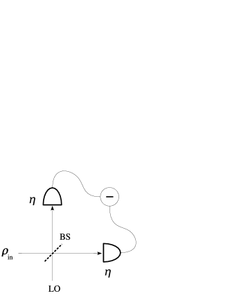
Figure 2: Scheme of the homodyne receiver. The signal to be processed is mixed at a balanced beam splitter with a highly excited coherent reference state, usually referred to as the local oscillator (LO). Then, the difference photocurrent is measured at the output. In the ideal case $\rho_{\rm in}=\rho_{\mu}=|\mu\rangle\langle\mu|$, $\mu=0,\alpha$, and the the detection efficiency is $\eta=1$. In presence of noise, $\rho_{\rm in}$ is given by equation (18) and $\eta<1$.

An alternative receiver for single mode communication is provided by homodyne detection, which offers the advantage of amplification from a local oscillator, avoiding the need of single-photon avalanche photodetectors [20]. A schematic diagram of the balanced homodyne detection is shown in figure 2: here the signal interferes with a local oscillator (LO), i.e. a highly excited coherent state, in a balanced BS [this corresponds to put $\phi=\pi/4$ in equation (4)]. After the BS the two modes are detected and the difference photocurrent is electronically formed. For unit quantum efficiency of photodiodes, the POVM of the detector is $\Pi_{x}=|x\rangle\langle x|$, with

$$|x\rangle=\left(\frac{2}{\pi}\right)^{1/4}{\rm e}^{-x^{2}}\sum_{n=0}^{\infty}\frac{H_{n}(\sqrt{2}x)}{\sqrt{n!\,2^{n}}}\,|n\rangle$$ (30)

being an eigenstate of the quadrature operator $x=\frac{1}{2}(a+a^{\dagger})$ of the measured mode. In equation (30) $H_{n}(x)$ denotes the $n$-th Hermite polynomials. The probability density $p(x|\mu)$ of obtaining the outcome $x$ from homodyne detection with input state $|\mu\rangle$, $\mu=0,\alpha$, is

$$p(x|\mu)={\rm Tr}\{|\mu\rangle\langle\mu|\,\Pi_{x}\}=\sqrt{\frac{2}{\pi}}\,\exp\{-2(x-\mu)^{2}\}\>.$$ (31)

In equation (31) $\alpha$ is assumed as real. Equivalently, if $\alpha\in\mathbb{C}$, the same result may be obtained by measuring a suitable quadrature $x_{\varphi}=\frac{1}{2}(a^{{\dagger}}e^{\varphi}+ae^{-\varphi})$, with $\varphi={\rm arg}(\alpha)$. The minimum error probability for the homodyne receiver is given by

$$H_{{\rm e}} = \frac{1}{2}\left\{H(0|\alpha)+H(\alpha|0)\right\}$$ (32)

$$= \frac{1}{2}\left\{\int_{-\infty}^{\alpha/2}{\rm d}x\,p(x|\alpha)+\int_{\alpha/2}^{+\infty}{\rm d}x\,p(x|0)\right\}$$

$$= \frac{1}{2}\left\{1-{\rm Erf}\left[\sqrt{N}\right]\right\},$$

where $H(0|\alpha)$ and $H(\alpha|0)$ are the probabilities of inferring the signal $|0\rangle$ when it is actually $|\alpha\rangle$ and vice versa. ${\rm Erf}[a]=\frac{2}{\sqrt{\pi}}\int_{0}^{a}{\rm d}\zeta\,{\rm e}^{-\zeta^{2}}$ denotes the error function. Notice that, in general, the error probability depends on the choice of a threshold parameter $\Lambda$, i.e.

$$H_{{\rm e}}(\Lambda) = \frac{1}{2}\left\{\int_{-\infty}^{\Lambda}{\rm d}x\,p(x|\alpha)+\int_{\Lambda}^{+\infty}{\rm d}x\,p(x|0)\right\}$$ (33)

$$= \frac{1}{2}\left\{1-\frac{1}{2}\left({\rm Erf}[\sqrt{2}\Lambda]+{\rm Erf}[\sqrt{2}(\alpha-\Lambda)]\right)\right\}\>.$$

In our case this probability is minimized when $\Lambda=\alpha/2$, thus leading to the result in equation (32). In the limit $N\gg 1$, equation (32) reduces to

$$H_{{\rm e}}\approx\frac{{\rm e}^{-N}}{2\sqrt{\pi N}}\,.$$ (34)

Homodyne detection provides a better discrimination of the signals than direct detection, i.e. $H_{\rm e}<K_{\rm e}$ if the energy of the channel is below a threshold that monotonically increases as the transmissivity of the BS in the receiver decreases. In the limit of $\tau\rightarrow 1$ in direct detection, we have $H_{\rm e}<K_{\rm e}$ for $N\lesssim 0.77$ while, as an example, for $\tau=0.9$ we have $H_{\rm e}<K_{\rm e}$ for $N\lesssim 1.10$.

2.4 Homodyne detection - Noise in propagation and detection

As already shown in section 2.2, if noise affects the propagation of the signal, the state arriving at the homodyne receiver is no longer a pure state, and is given in equation (18). Moreover, when also homodyne detection is not ideal, the POVM of the receiver is a Gaussian convolution of the ideal POVM

$$\Pi_{x}(\eta)=\frac{1}{\sqrt{2\pi\sigma_{\eta}^{2}}}\int{\rm d}y\,\exp\left\{-\frac{(y-x)^{2}}{2\sigma_{\eta}^{2}}\right\}\,\Pi_{y}\,,$$ (35)

where $\sigma_{\eta}^{2}=(1-\eta)/(4\eta)$, and $\eta$ is the quantum efficiency of both photodiodes involved in homodyning (we assume that they have the same quantum efficiency). The Wigner function of $\Pi_{x}(\eta)$ is given by

$$W[\Pi_{x}(\eta)](\zeta) \equiv W[\Pi_{x}(\eta)](\hbox{Re}[\zeta])$$ (36)

$$= \frac{1}{\sqrt{2\pi\sigma_{\eta}^{2}}}\,\exp\left\{-\frac{(\hbox{Re}[\zeta]-x)^{2}}{2\sigma_{\eta}^{2}}\right\}\,.$$

Taking into account all the sources of noise, the probability density of equation (31) becomes

$$p_{\eta,\Gamma,M}(x|\mu) = {\rm Tr}\{D(\mu^{\prime})\,\nu_{M^{\prime}}\,D^{{\dagger}}(\mu^{\prime})\,\Pi_{x}(\eta)\}\,,$$ (37)

with $\mu^{\prime}=\mu\>{\rm e}^{-\frac{1}{2}\Gamma t}$, $\mu=0,\alpha$, and $\nu_{M^{\prime}}$ given by equation (19). In this way, using the Wigner functions and thanks to equation (21), the error probability reads as follows

$$H_{{\rm e}}(N,\eta,\Gamma,M)=\frac{1}{2}\left\{1-{\rm Erf}\left[\frac{\sqrt{\eta N}\,{\rm e}^{-\frac{1}{2}\Gamma t}}{\sqrt{1+2\eta M(1-{\rm e}^{-\Gamma t})}}\right]\right\}\,,$$ (38)

which, in the limit $\eta N\>{\rm e}^{-\Gamma t}\gg 1+2\eta M(1-{\rm e}^{-\Gamma t})$, reduces to

$$H_{{\rm e}}(N,\eta,\Gamma,M)\approx\frac{\sqrt{1+2\eta M(1-{\rm e}^{-\Gamma t})}\,\exp\left\{-\frac{\eta N\>{\rm e}^{-\Gamma t}}{1+2\eta M(1-{\rm e}^{-\Gamma t})}\right\}}{2\sqrt{\pi\eta N}\>{\rm e}^{-\frac{1}{2}\Gamma t}}\,.$$ (39)

In the next section we compare $H_{\rm e}$ with the corresponding error probability in direct detection.

2.5 Direct vs homodyne detection

In order to individuate the working regimes where homodyne detection provides better performances, i.e. lower error probability than direct detection, we define the following quantity

$$A_{{\rm e}}(N,\eta_{{\rm ken}},\eta_{{\rm hom}},\Gamma,M)=1-\frac{H_{{\rm e}}(N,\eta_{{\rm hom}},\Gamma,M)}{K_{{\rm e}}(N,\eta_{{\rm ken}},\Gamma,M)}\,,$$ (40)

where $\eta_{{\rm ken}}$ and $\eta_{{\rm hom}}$ are the on/off and homodyne detection efficiencies, respectively. When $A_{{\rm e}}>0$ homodyne receiver’s error probability is the lowest. In figure 3 we plot $A_{{\rm e}}$ as a function of the energy of the channel $N$ for different values of the other parameters. For given values of $\eta_{{\rm ken}}$, $\eta_{{\rm hom}}$, $\Gamma$ and $M$ we have two different thresholds for the energy channel, namely $N^{\rm(hom)}_{{\rm th},j}(\eta_{{\rm ken}},\eta_{{\rm hom}},\Gamma,M)$, $j=1,2$, such that $A_{{\rm e}}=0$. For $N\leq N^{\rm(hom)}_{{\rm th},1}$ we have a small interval where homodyne detection should be preferred to direct one; as $N$ increases, we find a window ($N^{\rm(hom)}_{{\rm th},1}<N\leq N^{\rm(hom)}_{{\rm th},2}$), where $H_{{\rme}}>K_{{\rm e}}$ and, finally, a last region for $N>N^{\rm(hom)}_{{\rm th},2}$ where homodyne detection returns to be definitely better (see table 2). This result is due to the presence of thermal noise (i.e. $T\neq 0$). In fact, as one can easily see from equations (29) and (39) one has, independently on $M$

$$\lim_{N\rightarrow\infty}K_{{\rm e}}(N,\eta_{{\rm ken}},\Gamma,M) = \frac{\eta_{{\rm ken}}M(1-{\rm e}^{-\Gamma t})\cos^{2}\phi}{2[1+\eta_{{\rm ken}}M(1-{\rm e}^{-\Gamma t})\cos^{2}\phi]}\,,$$ (41)

$$\lim_{N\rightarrow\infty}H_{{\rm e}}(N,\eta_{{\rm hom}},\Gamma,M) = 0\,.$$ (42)

In summary, homodyne detection provides better results for either small or large values of the channel energy $N$, whereas for intermediate values of $N$ the optimal choice is represented by direct detection. The width of this intermediate region decreases as the noise increases, i.e. as the value of both $\Gamma$ and $M$ increases. We therefore conclude that homodyne detection is a more robust receiver in presence of noise. As concern quantum efficiency, we have, as one may expect, that the performances of each detector improves increasing the corresponding $\eta$.

3 Binary communication in entangled channels

Entanglement is a key feature of quantum mechanics. The quantum nonlocality due to entanglement has been, in the last decade, harnessed for practical use in the quantum information technology [21, 22]. Entanglement has become an essential resource for quantum computing [22], quantum teleportation [23], dense coding [15], and secure cryptographic protocols [22] as well as for improving optical resolution [24], spectroscopy [25], and general quantum measurements [26]. Here we show how entanglement, and in particular entangled states that can be realized by current optical technology, can be used to improve binary communications, i.e. to reduce the error probability at fixed energy of the channel.

3.1 Heterodyne detection - Ideal case

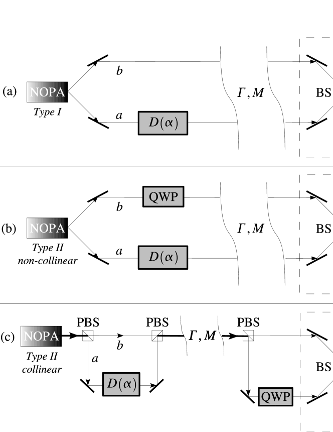
Figure 4: Schematic diagrams of possible implementations of entanglement based binary optical communication with TWB and multiport homodyne detection. In (a): TWB are produced by spontaneous downconversion in a type I nondegenerate optical parametric amplifier (NOPA). In this case the two modes have the same polarization. A displacement $D(\alpha)$ is applied to mode $a$ and then the signal is transmitted toward a multiport homodyne receiver. In (b): TWB are produced by spontaneous downconversion in a noncollinear type II NOPA. In this case the two TWB modes have different wave-vector and orthogonal polarizations. A displacement $D(\alpha)$ is applied to mode $a$, while a quarter wave plate (QWP) rotates the polarization of the mode $b$ so that they become same polarized. After the propagation, the two modes are detected as before. In (c): TWB are produced by spontaneous downconversion in a collinear type II NOPA. In this case the two TWB modes have the same wave-vector and orthogonal polarizations. A first polarizer beam splitter (PBS) reflects the mode $a$, which is displaced by $D(\alpha)$, and transmits mode $b$; the two modes are then recombined in a second PBS and transmitted. Before detection another PBS reflects mode $a$ toward a QWP that changes its polarization to the same of mode $b$. During propagation modes are subjected to losses (at rate $\Gamma$) and thermal noise (parameter $M$). The detector efficiency is $\eta$.

Binary optical communication assisted by entanglement may be implemented using twin-beam (TWB) state of two modes of radiation [14]. Schematic diagrams of some possible implementations are given in figure 4. In the Fock basis the TWB writes as follows

$$|\lambda\rangle\rangle=\sqrt{1-\lambda^{2}}\,\sum_{n}\,\lambda^{n}\,|n\rangle|n\rangle\>,$$ (43)

where $|\lambda|<1$ and, without loss of generality, it may be taken as real ($\lambda$ is sometimes referred to as the TWB parameter). TWB is the maximally entangled state (for a given, finite, value of energy) of two modes of radiation. It can be produced either by mixing two single-mode squeezed vacuum (with orthogonal squeezing phases) in a balanced beam splitter [23] or, from the vacuum, by spontaneous downconversion in a nondegenerate optical parametric amplifier (NOPA) made either by type I or type II second order nonlinear crystal [27]. Referring to the amplification case, the evolution operator reads as $U_{r}=\exp{\left\{r\left(a^{\dagger}b^{\dagger}-ab\right)\right\}}$ where the “gain” $r$ is proportional to the interaction-time, the nonlinear susceptibility, and the pump intensity. We have $\lambda=\tanh r$, whereas the number of photons of TWB is given by $N_{\lambda}=2\sinh^{2}r=2\lambda^{2}/(1-\lambda^{2})$.

The two signals to be discriminated in a AMK encoding are given by $|\psi_{0}\rangle\rangle=|\lambda\rangle\rangle$ and $|\psi_{\alpha}\rangle\rangle=[D_{a}(\alpha)\otimes\mathbb{I}]|\lambda\rangle\rangle$, where the displacement operator $D_{a}(\alpha)$ is acting on one of the modes, say $a$, of the TWB. The energy of the TWB channel, i.e. the average photon number per use, is given by $N=\frac{1}{2}{\rm Tr}\{(a^{{\dagger}}a\otimes\mathbb{I}+\mathbb{I}\otimes b^{{\dagger}}b)(\rho_{0}+\rho_{\alpha})\}=N_{\lambda}+\frac{1}{2}|\alpha|^{2}$, with $\rho_{0}=|\psi_{0}\rangle\rangle\langle\langle\psi_{0}|$ and $\rho_{\alpha}=|\psi_{\alpha}\rangle\rangle\langle\langle\psi_{\alpha}|$.

The error probability for the ideal discrimination between the two states $|\psi_{0}\rangle\rangle$ and $|\psi_{\alpha}\rangle\rangle$ reads as follows

$$Q_{{\rm e}} = \frac{1-\sqrt{1-|\langle\langle\psi_{0}|\psi_{\alpha}\rangle\rangle|^{2}}}{2}$$ (44)

$$= \frac{1-\sqrt{1-\exp\{-2N(1-\beta)(1+\beta N)\}}}{2},$$

where $\beta\equiv N_{\lambda}/N$ is the fraction of the channel energy that is used to establish the entanglement between the two modes. Probability (44) is minimum for $\beta=(N-1)/2N$, when $N\geq 1$, and for $\beta=0$ when $0<N<1$. In summary one has

$$Q_{{\rm e}}=P_{{\rm e}} (N<1)$$ (45)

$$Q_{{\rm e}}=\frac{1-\sqrt{1-\exp\{-\frac{1}{2}(1+N)^{2}\}}}{2}\qquad (N\geq 1)\>,$$ (46)

where $P_{\rm e}$, given in equation (2), is the minimum error probability for single-mode AMK signals. Equations (45) and (46) say that $Q_{{\rm e}}\leq P_{{\rm e}}$ $\forall N$, i.e. that the use of entanglement, at least in the ideal situation considered so far, never increases the error probability, and it is convenient if the photon number of the channel is larger than one.

In order to see whether this result holds also in practice, it is necessary to find out a realistic receiver able to discriminate $|\psi_{0}\rangle\rangle$ and $|\psi_{\alpha}\rangle\rangle$, and to discuss its performances in presence of noise. As concern detectors, we may use either multiport homodyne detection, if the two modes have the same frequencies [28], or heterodyne detection otherwise [29]. Both these detection schemes allow the measurement of the real and the imaginary part of the complex operator $Z=a-b^{{\dagger}}$. In figure 4 we have referred to to eight-port homodyne detection; however all the results also hold for other multiport homodyne schemes and for heterodyne detection. Each outcome from the measurement of $Z$ is a complex number $z$ and the POVM of receiver is given by $\Pi_{z}=\frac{1}{\pi}|z\rangle\rangle\langle\langle z|$, where

$$|z\rangle\rangle=[D_{a}(z)\otimes\mathbb{I}]\sum_{n}|n\rangle|n\rangle=[\mathbb{I}\otimes D_{b}(-z^{*})]\sum_{n}|n\rangle|n\rangle\>.$$

As already discussed for homodyne detection, we may take the amplitude $\alpha$ as real. In this case a suitable inference rule to infer the input state from $Z$-data involves the real part of the outcome as follows

$${\rm Re}[z]>\Lambda\Longrightarrow|\psi_{\alpha}\rangle\rangle\>,$$

where $\Lambda$ is a threshold value, which should be chosen such to minimize the probability of error

$$R_{{\rm e}}=\frac{1}{2}\left\{R(0|\alpha)+R(\alpha|0)\right\}\>,$$ (47)

where $R(0|\alpha)$ and $R(\alpha|0)$ are the probabilities to detect $|\psi_{0}\rangle\rangle$ when $|\psi_{\alpha}\rangle\rangle$ was sent and vice versa. The heterodyne distribution conditioned to a displacement $D(\alpha)=D_{a}(\alpha)\otimes\mathbb{I}$ is given by the probability density

$$r(z|\mu)=|\langle\langle z|D(\mu)|\lambda\rangle\rangle|^{2}=\frac{1}{\pi\Delta_{\lambda}^{2}}\exp\left\{-\frac{|\mu-z|^{2}}{\Delta_{\lambda}^{2}}\right\}$$ (48)

with $\mu=0,\alpha$, and $\Delta_{\lambda}^{2}=(1-\lambda)/(1+\lambda)=(\sqrt{N_{\lambda}+2}-\sqrt{N_{\lambda}})/(\sqrt{N_{\lambda}+2}+\sqrt{N_{\lambda}})$. Therefore we have

$$R(0|\alpha) = \int_{-\infty}^{\Lambda}{\rm d}x\int_{-\infty}^{\infty}{\rm d}y\,r(z|\alpha)$$ (49)

$$R(\alpha|0) = \int_{\Lambda}^{\infty}{\rm d}x\int_{-\infty}^{\infty}{\rm d}y\,r(z|0),$$ (50)

where $z=x+iy$, and the error probability (47) becomes

$$R_{{\rm e}}=\frac{1}{2}\left\{1-\frac{1}{2}\left({\rm Erf}\left[\frac{\Lambda}{\Delta_{\lambda}}\right]+{\rm Erf}\left[\frac{\alpha-\Lambda}{\Delta_{\lambda}}\right]\right)\right\}.$$ (51)

$R_{\rm e}$ in equation (51) is minimized by choosing $\Lambda=\alpha/2$, thus leading to

$$R_{{\rm e}}=\frac{1}{2}\left\{1-{\rm Erf}\left[\frac{1}{2}\frac{\alpha}{\Delta_{\lambda}}\right]\right\}\>.$$

At this point, the error probability $R_{{\rm e}}$ can be further minimized by tuning the entanglement fraction $\beta$. By substituting the expression for the amplitude $\alpha=\sqrt{2N(1-\beta)}$ and the variance $\Delta_{\lambda}^{2}=(\sqrt{\beta N+2}-\sqrt{\beta N})/(\sqrt{\beta N+2}+\sqrt{\beta N})$, we obtain

$$R_{{\rm e}}=\frac{1}{2}\left\{1-{\rm Erf}\left[\frac{1}{2}\sqrt{\frac{2N(1-\beta)(\sqrt{\beta N+2}+\sqrt{\beta N})}{\sqrt{\beta N+2}-\sqrt{\beta N}}}\right]\right\}.$$ (52)

The optimal entanglement fraction, which minimizes $R_{{\rm e}}$, is given by

$$\beta_{{\rm opt}}(N)=\frac{N}{2(1+N)}\,.$$ (53)

In figure 5 we report the resulting expression for the error probability, compared with the corresponding single-mode error probabilities $K_{\rm e}$ and $H_{\rm e}$. As the channel energy increases, the heterodyne error probability decreases more rapidly than the single-mode ones. For a channel energy $N\lesssim 0.79$ homodyne detection gives the best performances, whereas as the channel energy increases the best results are obtained by direct detection ($0.79\lesssim N\lesssim 4.46$) and heterodyne detection ($N\gtrsim 4.46$). These results are summarized in table 1. Notice that for $N\gtrsim 5.2$ we have $R_{\rm e}<P_{\rm e}$, i.e. TWB heterodyne channel provides better performance even than ideal single-mode channel.

3.2 Heterodyne detection - Noise in propagation and detection

At first we consider the noise occurring during the propagation of the TWB or its displaced version. This is described as the coupling of each mode of the TWB with a thermal bath of oscillators at temperature $T$. The dynamics is then described by the two-mode Master equation

$$\frac{{\rm d}\rho_{t}}{{\rm d}t}=\left\{\Gamma(1+M)L[a]+\Gamma(1+M)L[b]+\Gamma ML[a^{{\dagger}}]+\Gamma ML[b^{{\dagger}}]\right\}\rho_{t}\,,$$ (54)

where $\rho_{t}$ is the density matrix of the bipartite system and the other parameters are as in equation (12). The terms proportional to $L[a]$ and $L[b]$ describe the losses, whereas the terms proportional to $L[a^{{\dagger}}]$ and $L[b^{{\dagger}}]$ describe a linear phase-insensitive amplification process. Of course, the dissipative dynamics of the two modes are independent on each other.

The Master equation (54) can be reduced to a Fokker-Planck equation for the two-mode Wigner function $W_{\mu}(\xi,\zeta)\equiv W[\rho_{\mu}](\xi,\zeta)$ of the system,

$$W_{\mu}(\xi,\zeta)\equiv\frac{1}{\pi^{4}}\int\!{\rm d}^{2}\chi\int\!{\rm d}^{2}\lambda\,{\rm e}^{\xi\chi^{*}-\xi^{*}\chi}\,{\rm e}^{\zeta\lambda^{*}-\zeta^{*}\lambda}\,{\rm Tr}\left\{\rho_{\mu}\,D_{a}(\chi)\otimes D_{b}(\lambda)\right\}\,,$$ (55)

where $\xi,\zeta\in\mathbb{C}$, $\rho_{\mu}=|\psi_{\mu}\rangle\rangle\langle\langle\psi_{\mu}|$, $\mu=0,\alpha$, and $D_{j}$, $j=a,b$, is the displacement operator acting on mode $j$. Using the differential representation of the superoperator in equation (54), the corresponding Fokker-Planck equation reads as follows

$$\partial_{t}W_{\mu,t}(\xi,\zeta)=\frac{\Gamma}{2}\left\{\sum_{j=1}^{2}\left(\partial_{x_{j}}x_{j}+\partial_{y_{j}}y_{j}\right)+\left(2M+1\right)\sum_{j=1}^{2}\left(\partial_{x_{j}x_{j}}^{2}+\partial_{y_{j}y_{j}}^{2}\right)\right\}W_{\mu,t}(\xi,\zeta)\,,$$ (56)

where $\xi=x_{1}+iy_{1}$, $\zeta=x_{2}+iy_{2}$. The solution of equation (56) can be written as

$$W_{\mu,t}(\xi,\zeta)=\int\!\!\!\int\!{\rm d}x^{\prime}_{1}{\rm d}y^{\prime}_{1}\int\!\!\!\int\!{\rm d}x^{\prime}_{2}{\rm d}y^{\prime}_{2}\,W_{\mu,0}(x^{\prime}_{1},y^{\prime}_{1};x^{\prime}_{2},y^{\prime}_{2})\times\prod_{j=1}^{2}G_{t}(x_{j}|x^{\prime}_{j})G_{\tau}(y_{j}|y^{\prime}_{j})\,,$$ (57)

where $W_{\mu,0}(x^{\prime}_{1},y^{\prime}_{1};x^{\prime}_{2},y^{\prime}_{2})$ is the Wigner function at $t=0$ and the Green’s functions $G_{t}(x_{j}|x^{\prime}_{j})$ are given in equation (16). The Wigner function $W_{\mu,0}(x_{1},y_{1};x_{2},y_{2})$ before the propagation is given by (remind that $\mu=0,\alpha$, and $\alpha$ is taken as real)

$$W_{\mu,0}=\frac{\exp\left\{-\frac{(x_{1}+x_{2}-\mu)^{2}}{4\sigma_{+}^{2}}-\frac{(y_{1}+y_{2})^{2}}{4\sigma_{-}^{2}}-\frac{(x_{1}-x_{2}-\mu)^{2}}{4\sigma_{-}^{2}}-\frac{(y_{1}-y_{2})^{2}}{4\sigma_{+}^{2}}\right\}}{(2\pi\sigma_{+}^{2})(2\pi\sigma_{-}^{2})}\>$$ (58)

with

$$\sigma_{\pm}^{2}=\frac{1}{4}(\Delta_{\lambda}^{2})^{\mp 1}\>.$$ (59)

$\Delta_{\lambda}^{2}$ being as in equation (48). Since $W_{\alpha,0}$ is Gaussian, the Wigner function $W_{\alpha,t}$ can be easily evaluated. One has

$$W_{\mu,t}=\frac{\exp\left\{-\frac{(x_{1}+x_{2}-\mu\>{\rm e}^{-\frac{1}{2}\Gamma t})^{2}}{4\Sigma_{+}^{2}}-\frac{(y_{1}+y_{2})^{2}}{4\Sigma_{-}^{2}}-\frac{(x_{1}-x_{2}-\mu\>{\rm e}^{-\frac{1}{2}\Gamma t})^{2}}{4\Sigma_{-}^{2}}-\frac{(y_{1}-y_{2})^{2}}{4\Sigma_{+}^{2}}\right\}}{(2\pi\Sigma_{+}^{2})(2\pi\Sigma_{-}^{2})}\,$$ (60)

where

$$\Sigma_{\pm}^{2}=D^{2}+\sigma_{\pm}^{2}{\rm e}^{-\Gamma t}\,.$$ (61)

The signals described by the Wigner functions of equation (60) correspond to entangled states if $\Sigma_{-}^{2}\leq\frac{1}{4}$ [30, 31, 32], i.e. if

$${\rm e}^{-2r}\equiv 1+N_{\lambda}-\sqrt{N_{\lambda}(N_{\lambda}+2)}\leq{\rm e}^{\Gamma t}-(2M+1)({\rm e}^{\Gamma t}-1)\,.$$

If no thermal noise occurs ($M=0$), entanglement is present at any time, whereas for $M\neq 0$ the survival time is given by

$$t_{\rm s}=\frac{1}{\Gamma}\log\left(1+\frac{\sqrt{N_{\lambda}(N_{\lambda}+2)}-N_{\lambda}}{2M}\right)\;,$$ (62)

and the corresponding survival entanglement fraction $\beta_{\rm s}(N,\Gamma,M,t)$ reads as follows

$$\beta_{\rm s}(N,\Gamma,M,t)=\frac{2M^{2}({\rm e}^{\Gamma t}-1)^{2}}{N[1-2N({\rm e}^{\Gamma t}-1)]}\;.$$ (63)

The meaning of equation (63) is that if the initial entanglement fraction is above threshold, i.e. $\beta>\beta_{\rm s}$, the state remains not separable after propagation. Besides propagation noise, one should take into account detection efficiency at the heterodyne receiver. In this case the POVM of the detector is a Gaussian convolution of the ideal POVM

$$\Pi_{z}(\eta)=\frac{1}{\pi\sigma_{\eta}^{2}}\int\!{\rm d}^{2}\beta\,\exp\left\{-\frac{|z-\beta|^{2}}{\sigma_{\eta}^{2}}\right\}\,\Pi_{\beta}\,,$$ (64)

with $\sigma_{\eta}^{2}=(1-\eta)/\eta$. The Wigner function associated to the POVM (64) is given by

$$W[\Pi_{z}(\eta)](x_{1},y_{1};x_{2},y_{2})=\frac{\exp\left\{-\frac{(x_{1}-x_{2}-\hbox{Re}[z])^{2}}{\sigma_{\eta}^{2}}-\frac{(y_{1}+y_{2}-\hbox{Im}[z])^{2}}{\sigma_{\eta}^{2}}\right\}}{\pi\sigma_{\eta}^{2}}$$ (65)

and the corresponding heterodyne distribution $r_{\eta,\Gamma,M}(z|\alpha)$ by

$$r_{\eta,\Gamma,M}(z|\alpha)=\frac{1}{\pi\Delta_{\eta,\Gamma,M}^{2}}\exp\left\{-\frac{|z-\alpha\>{\rm e}^{-\frac{1}{2}\Gamma t}|^{2}}{\Delta_{\eta,\Gamma,M}^{2}}\right\}\,,$$ (66)

with

$$\Delta_{\eta,\Gamma,M}^{2}=4\Sigma_{-}^{2}+\sigma_{\eta}^{2}=(1+2M)(1-{\rm e}^{-\Gamma t})+\Delta_{\lambda}^{2}\,{\rm e}^{-\Gamma t}+\frac{1-\eta}{\eta}\,.$$ (67)

The error probability, as defined in the previous Sections, already taking into account that the optimal threshold is given by $\Lambda=\frac{1}{2}\alpha\>{\rm e}^{-\frac{1}{2}\Gamma t}$, reads as follows

$$R_{{\rm e}}(N,\eta,\Gamma,M)=\frac{1}{2}\left\{1-{\rm Erf}\left[\frac{1}{2}\frac{\alpha\>{\rm e}^{-\frac{1}{2}\Gamma t}}{\Delta_{\eta,\Gamma,M}}\right]\right\}\,,$$ (68)

and the optimal entanglement fraction $\beta_{{\rm opt}}(N,\eta,\Gamma,M,t)\equiv\beta_{{\rm opt}}$, which minimizes the error probability, is obtained after some algebra. One has

$$\beta_{{\rm opt}}=\frac{\eta^{2}N{\rm e}^{-2\Gamma t}}{1+A(N,\eta,\Gamma,M,t)+B(N,\eta,\Gamma,M)\sqrt{1+C(N,\eta,\Gamma,M,t)}}\,,$$ (69)

where

$$A(N,\eta,\Gamma,M) = \eta N{\rm e}^{-\Gamma t}(2-\eta\>{\rm e}^{-\Gamma t})+4f(N,\eta,\Gamma,M)\,,$$ (70)

$$B(N,\eta,\Gamma,M) = 1+\eta N{\rm e}^{-\Gamma t}+2\eta M(1-{\rm e}^{-\Gamma t})\,,$$ (71)

$$C(N,\eta,\Gamma,M) = 2\eta N{\rm e}^{-\Gamma t}(1-\eta\>{\rm e}^{-\Gamma t})+2f(N,\eta,\Gamma,M)\,,$$ (72)

with

$$f(N,\eta,\Gamma,M)=\eta M(1-{\rm e}^{-\Gamma t})[1+\eta N{\rm e}^{-\Gamma t}+\eta M(1-{\rm e}^{-\Gamma t})]\,.$$ (73)

As a matter of fact, the optimal entanglement fraction depends on the noise parameters of the channel. In particular, it can be seen that $\beta_{{\rm opt}}$ decreases as $\Gamma$ and $M$ increase and $\eta$ decreases. In other words, as the channel becomes more noisy, the entanglement becomes less useful. In figure 6 we report $\beta_{{\rm opt}}$ for fixed detection efficiency and $\beta_{s}$ as functions of the channel number of photons for different values of the other parameters.

3.3 Direct vs heterodyne detection

Heterodyne detection provides better performance than direct detection when the quantity

$$B_{{\rm e}}(N,\eta_{{\rm ken}},\eta_{{\rm het}},\Gamma,M)=1-\frac{R_{{\rm e}}(N,\eta_{{\rm het}},\Gamma,M)}{K_{{\rm e}}(N,\eta_{{\rm ken}},\Gamma,M)}\,,$$ (74)

is positive, i.e. $R_{\rm e}<K_{\rm e}$. In equation (74) $\eta_{\rm ken}$ and $\eta_{\rm het}$ are the on/off and heterodyne detection efficiencies, respectively. In figure 7 we plot $B_{\rm e}$ as a function of channel energy $N$ for different values of the other parameters. Three regions of interest can be identified, since, as in the case of homodyne detection, for given values of $\eta_{{\rm ken}}$, $\eta_{{\rm het}}$, $\Gamma$ and $M$ we have two different thresholds for the energy channel, namely $N^{\rm(het)}_{{\rm th},j}(\eta_{{\rm ken}},\eta_{{\rm het}},\Gamma,M)$, $j=1,2$, such that $B_{{\rm e}}=0$. Heterodyne error probability is the smallest in a small region for $N\leq N^{\rm(het)}_{{\rm th},1}$ and for large values of the channel energy ($N>N^{\rm(het)}_{{\rm th},2}$), whereas in an intermediate interval of energy values ($N^{\rm(het)}_{{\rm th},1}<N\leq N^{\rm(het)}_{{\rm th},2}$) the best results are obtained by direct detection (see table 3).

As for the homodyne detection, heterodyne receiver provides better results for either small or large values of the channel energy $N$, whereas for the intermediate region, whose width depends on $\Gamma$, $M$ and $\eta$ as in the case of $A_{\rm e}$, direct detection should be preferred.

3.4 Heterodyne vs homodyne detection

Since the channel energy intervals where heterodyne and homodyne detection should be preferred to direct one are quite similar, it is useful to introduce the function

$$C_{{\rm e}}(N,\eta,\eta,\Gamma,M)=1-\frac{R_{{\rm e}}(N,\eta,\Gamma,M)}{H_{{\rm e}}(N,\eta,\Gamma,M)}\,,$$ (75)

which is positive when $R_{\rm e}<H_{\rm e}$. As one can see in figure 8, there exists a threshold $N_{{\rm th}}(\eta,\Gamma,M)$ on the channel energy $N$ such that if $N>N_{{\rm th}}$ then $R_{\rm e}<H_{\rm e}$ (see table 4). Notice that the homodyne and heterodyne detection efficiencies have the same value. In figure 9 we plot $N_{{\rm th}}$ for different physical situation. The threshold increases with increasing noise either in the propagation or in the detection stage. For a channel energy above the threshold the use of entanglement improves the communication performances.

4 Conclusions

In this paper we have analyzed binary communication in single-mode and entangled quantum noisy channels. We took into account different kind of noise that may occur, i.e. losses and thermal noise during propagation, non unit quantum efficiency of detectors during the measurement stage.

As concern single mode communication, we found that, in presence of noise, homodyne detection is a more robust receiver when compared to direct detection. In particular, homodyne detection achieves a smaller error probability for either small or large values of the energy of the channel, whereas for intermediate values direct detection should be preferred.

We then considered an entanglement based quantum channel build by amplitude modulated twin-beam and multiport homodyne detection. As for the homodyning, heterodyne detection should be preferred to direct detection for either small or large values of the energy of the channels. On the other hand the comparison between the performances of heterodyne and homodyne detection shows that there exists a threshold on the channel energy, above which the error probability using entangled channels and heterodyning is the smallest. The threshold depends on the amount of noise, and increases as imperfections in propagation and detection become more relevant. We summarized our results in tables 1, 2, 3, and 4.

We conclude that entanglement is a useful resource to improve binary communication in presence of noise, especially in the large energy regime.

References

Channel energy	Best detector (channel)
$N\lesssim 0.79$	Homodyne (single mode)
$0.79\lesssim N\lesssim 4.46$	Direct (single mode)
$N\gtrsim 4.46$	Heterodyne (entangled)

Table 1: Comparison among direct, homodyne and heterodyne detection as a function of the channel energy when transmission and detection are ideal (see also figure 5).

Channel energy	Best detector (channel)
$N\leq N^{\rm(hom)}_{{\rm th},1}$	Homodyne (single mode)
$N^{\rm(hom)}_{{\rm th},1}<N\leq N^{\rm(hom)}_{{\rm th},2}$	Direct (single mode)
$N>N^{\rm(hom)}_{{\rm th},2}$	Homodyne (single mode)

Table 2: Comparison between direct and homodyne detection as a function of the channel energy in presence of noise during the transmission and detection stages. The thresholds $N^{\rm(hom)}_{{\rm th},j}(\eta_{\rm ken},\eta_{\rm hom},\Gamma,M)$, $j=1,2$, define three different regimes (see also figure 3).

Channel energy	Best detector (channel)
$N\leq N^{\rm(het)}_{{\rm th},1}$	Heterodyne (entangled)
$N^{\rm(het)}_{{\rm th},1}<N\leq N^{\rm(het)}_{{\rm th},2}$	Direct (single mode)
$N>N^{\rm(het)}_{{\rm th},2}$	Heterodyne (entangled)

Table 3: Comparison between direct and heterodyne detection as a function of the channel energy in presence of noise during the transmission and detection stages. The thresholds $N^{\rm(het)}_{{\rm th},j}(\eta_{\rm ken},\eta_{\rm het},\Gamma,M)$, $j=1,2$, define three different regimes (see also figure 7).

Channel energy	Best detector (channel)
$N\leq N_{{\rm th}}$	Homodyne (single mode)
$N>N_{{\rm th}}$	Heterodyne (entangled)

Table 4: Comparison between heterodyne and homodyne detection as a function of the channel energy in presence of noise during the transmission and detection stages. The threshold $N_{{\rm th}}(\eta,\Gamma,M)$ defines two different regimes (see also figure 8).

Figure 3: Plots of $A_{{\rm e}}(N,\eta_{{\rm ken}},\eta_{{\rm hom}},\Gamma,M)$, defined in equation (40), as a function of $N$ for different values of $\Gamma t$ and $M$. The on/off and homodyne detection efficiencies are chosen to be the realistic values $\eta_{{\rm ken}}=0.95$ and $\eta_{{\rm hom}}=0.85$, respectively, and $\cos^{2}\phi=0.99$. The dashed line is $A_{{\rm e}}$ with $\Gamma,M=0$. In all the plots the solid lines correspond to (from bottom to top) $M=5\,10^{-3},5\,10^{-2},0.1$ and $0.2$, respectively, while $\Gamma t$ is: (a) $\Gamma t=10^{-2}$, (b) $\Gamma t=5\,10^{-2}$, (c) $\Gamma t=0.1$, (d) $\Gamma t=0.2$. The insets refer to the region $0<N<1$. When $A_{{\rm e}}>0$ one has $H_{{\rm e}}<K_{{\rm e}}$.

Figure 5: Linear-log plot of the error probabilities of direct ($K_{\rm e}$, dotted line), homodyne ($H_{\rm e}$, dot-dashed line) and heterodyne ($R_{\rm e}$, solid line) detection in the ideal case (absence of noise in propagation and detection) as functions of the channel energy $N$. We chose $\cos\phi^{2}=0.99$ for direct detection. As the channel energy increases, the heterodyne error probability decreases more rapidly than the single-mode ones. In the smaller pictures: magnification of the plot in the regions (a): $0<N<1$ and (b): $0<N<5$. For a channel energy $N\lesssim 0.79$ homodyne detection gives the best performances, whereas as the channel energy increases the best results are obtained by the direct ($0.79\lesssim N\lesssim 4.46$) and heterodyne detection ($N\gtrsim 4.46$).

Figure 6: Plots of the optimal entanglement fraction $\beta_{\rm opt}$ (solid lines) given in equation (69) and of the survival entanglement fraction $\beta_{\rm s}$ (dashed lines) given in equation (63) as a function of the channel energy $N$ for different values of $\Gamma$, $M$ and $\eta$. The plots (a2) and (b2) are magnifications of the regions $0<N<0.2$ of plots (a1) and (b1), respectively. In all the plots we put (from top to bottom for solid lines, from bottom to top for dashed lines) $M=5\,10^{-3},5\,10^{-2},0.1$ and $0.2$, respectively, whereas: (a1) $\eta=0.9$, $\Gamma t=10^{-1}$; (b1) $\eta=0.9$, $\Gamma t=2\,10^{-1}$. As the channel becomes more noisy, entanglement becomes less useful. Notice that for this choice of the parameters, when $N\gtrsim 0.056$ (a2) and $N\gtrsim 0.142$ (b2) the state arriving at the receiver is always non separable.

Figure 7: Plots of $B_{{\rm e}}(N,\eta_{{\rm ken}},\eta_{{\rm het}},\Gamma,M)$, defined in equation (74), as a function of $N$ for different values of $\Gamma t$ and $M$. The on/off and heterodyne detection efficiencies are chosen as $\eta_{{\rm ken}}=0.95$ and $\eta_{{\rm het}}=0.85$, respectively, and $\cos^{2}\phi=0.99$. The dashed line is $B_{{\rm e}}$ with $\Gamma,M=0$. In all the plots the solid lines correspond to (from bottom to top) $M=5\,10^{-3},5\,10^{-2},0.1$ and $0.2$, respectively, whereas $\Gamma t$ is: (a) $\Gamma t=10^{-2}$, (b) $\Gamma t=5\,10^{-2}$, (c) $\Gamma t=0.1$, (d) $\Gamma t=0.2$. The insets refer to the region $0<N<0.5$. When $B_{{\rm e}}>0$ one has $R_{{\rm e}}<K_{{\rm e}}$.

Figure 8: Plots of $C_{{\rm e}}(N,\eta,\Gamma,M)$, defined in equation (75), as a function of $N$ for different values of $\Gamma t$ and $M$. The heterodyne and homodyne detection efficiencies are chosen as $\eta_{=}0.85$. The dashed line is $C_{{\rm e}}$ with $\Gamma,M=0$. In all the plots the solid lines correspond to (from top to bottom) $M=5\,10^{-3},5\,10^{-2},0.1$ and $0.2$, respectively, whereas $\Gamma t$ is: (a) $\Gamma t=10^{-2}$, (b) $\Gamma t=5\,10^{-2}$, (c) $\Gamma t=0.1$, (d) $\Gamma t=0.2$. When $C_{{\rm e}}>0$ one has $R_{{\rm e}}<H_{{\rm e}}$.

Figure 9: $N_{{\rm th}}$ as a function of $\Gamma t$ for different values of the detection efficiency $\eta$ and the average number of thermal photons $M$. When $N>N_{{\rm th}}$ the error probability using entangled channels and heterodyne detection is less than the one obtained with a single-mode homodyne detection ($R_{{\rm e}}<H_{{\rm e}}$). The dashed line is $N_{{\rm th}}$ for $\eta=1$ and $M=0$, while the solid lines represent the threshold for (from right to left) $M=0,5\,10^{-2},0.1$ and $0.2$, respectively, whereas: (a) $\eta=1$, (b) $\eta=0.9$, (c) $\eta=0.8$ and (d) $\eta=0.7$.

References

• [1] C. W. Helstrom, J. W. S. Liu and J. P. Gordon, Proceedings of the IEEE 58, 1578 (1970).
• [2] C. W. Helstrom, Quantum Detection and Estimation Theory, Academic Press, New York, (1976).
• [3] M. G. A. Paris, Phys. Lett. A 217, 78 (1996).
• [4] This is a consequence of the fact that the set of displacement operators $\{D(\lambda)\}$, $\lambda\in\mathbb{C}$ represents a unitary irreducible representation the Weyl-Heisenberg group.
• [5] R. S. Kennedy, MIT Res. Lab. Electron. Quart. Prog. Rep. No. 108, 219 (1973).
• [6] S. J. Dolinar, MIT Res. Lab. Electron. Quart. Prog. Rep. No. 111, 115 (1973).
• [7] M. Sasaki, M. Ban and O. Hirota, Phys. Rev. A 54, 1691 (1996); M. Sasaki and O. Hirota, Phys. Rev. A 54, 2728 (1996); M. Sasaki and O. Hirota, Phys. Lett. A 224, 213 (1997).
• [8] Y. C. Eldar and G. D. Formey, IEEE Trans. Inform. Theory 47, 858 (2001).
• [9] M. Sasaki, A. Carlini and A. Chefles, J. Phys. A: Math. Gen. 34, 7017 (2001).
• [10] S. J. van Enk, Phys. Rev. A 66, 042308 (2002).
• [11] M. Sasaki, T. S. Usuda, O. Hirota and A. S. Holevo, Phys. Rev. A 53, 1273 (1995).
• [12] J. Mizuno, et al., Phys. Rev. A 65, 012315 (2001).
• [13] M. Sasaki, R. Momose and O. Hirota, Phys. Rev. A 55, 3222 (1997).
• [14] M. G. A. Paris in Quantum Communication Computing and Measurement V
ed. J. Shapiro and O. Hirota, Rinton Press (2003), p. 337; quant-ph/0210014.
• [15] M. Ban, J. Opt. B: Quantum and Semiclass. Opt. 2, 786 (2000).
• [16] P. Marian and T. A. Marian, Phys. Rev. A 47, 4474 (1993).
• [17] K. Cahill and R. Glauber, Phys. Rev. 177, 1857 (1969).
• [18] G. M. D’Ariano, C. Macchiavello, and M. G. A. Paris, in Quantum Communication and Measurement, ed. V. P. Belavkin et al., Plenum Press, New York and London (1995), p. 339.
• [19] D. Walls and G. Milburn, Quantum optics (Springer Verlag, Berlin, 1994).
• [20] H. P. Yuen and V. W. S. Chan, Opt. Lett. 8, 177 (1983); G. L. Abbas, V. W. S. Chan, S. T. Yee, Opt. Lett. 8, 419 (1983); IEEE J. Light. Tech. LT-3, 1110 (1985).
• [21] Introduction to Quantum Computation and Information, Ed. by H.-K. Lo, S. Popescu, T. Spiller, World Scientific (Singapore 1998).
• [22] I. L. Chuang and M. A. Nielsen, Quantum Information and Quantum Computation, Cambridge University Press (Cambridge UK 2000).
• [23] A. Furusawa et al., Science 282, 706 (1998).
• [24] M. I. Kolobov and C. Fabre, Phys. Rev. Lett. 85 3789 (2000).
• [25] B. E. A. Saleh, B. M. Jost, H.-B. Fei and M. C. Teich, Phys. Rev. Lett 80 3483 (1998).
• [26] G. M. D’Ariano, P. Lo Presti and M. G. A. Paris, Phys. Rev. Lett. 87, 270404 (2001).
• [27] O. Aytur and P. Kumar, Phys. Rev. Lett. 65, 1551 (1990).
• [28] N. G. Walker, J. Mod. Opt. 34, 15 (1987).
• [29] H. Yuen and J. Shapiro, IEEE Trans. Inform. Theory IT-26, 78 (1980).
• [30] M. G. A. Paris, Entangled light and applications in Progress in Quantum Physics Research, V. Krasnoholovets Ed., Nova Publisher, in press.
• [31] Lu-Ming Duan, G. Giedke, J. I. Cirac, and P. Zoller, Phys. Rev. Lett. 84 2722 (2000)
• [32] R. Simon, Phys. Rev. Lett. 84 2726 (2000)