Berry phase in a composite system

Abstract

The Berry phase in a composite system with only one subsystem being driven has been studied in this Letter. We choose two spin-$\frac{1}{2}$ systems with spin-spin couplings as the composite system, one of the subsystems is driven by a time-dependent magnetic field. We show how the Berry phases depend on the coupling between the two subsystems, and what is the relation between these Berry phases of the whole system and those of the subsystems.

Geometric phases in quantum theory attracted great interest since Berry berry shown that the state of a quantum system acquires a purely geometric feature in addition to the usual dynamical phase when it is varied slowly and eventually brought back to its initial form. The Berry phase has been extensively studied shapere ; thouless ; sun and generalized in various directions aharonov ; sjoqvist1 ; ericsson ; carollo ; fuentes , for example, geometric phases for mixed states sjoqvist1 , for open systemscarollo , and with a quantized field driving fuentes . In a recent paper sjoqvist2 , Sjöqvist calculated the geometric phase for a pair of entangled spins in a time-independent uniform magnetic field. This is an interesting development in holonomic quantum computer and in addition it shown how the prior entanglement in an initial state modify the Berry phase. This study was generalized tong1 to the case of spin pairs in a rotating magnetic field, the result shown that the geometric phase of the whole entangled bipartite system can be decomposed into a sum of geometric phases of the two subsystems, provided the evolution is cyclic.

Roughly speaking, entanglement may be created only via interactions or jointed measurements, thus how subsystem-subsystem interaction change the Berry phases of a composite system and those of the subsystems is of interest, from both sides of experimental and theoretical viewpoint. On the other hand, the Berry phase has very interesting applications, such as the implementation of quantum computation by geometric meansjones1 ; ekert ; falci ; wang . All systems for this purpose are composite, i.e., it at least consists of two subsystems with a direct coupling or being coupled through a third party. This again gives rise to questions of how the couplings among the subsystems changes the Berry phase of the composite system and what is the relation between these Berry phases of the composite system and those of the two subsystems.

In this Letter, we investigate the behavior of the Berry phase of two spin-$\frac{1}{2}$ systems with spin-spin couplings, one of the spin-$\frac{1}{2}$ is driven by a time-dependent magnetic field precessing around the z-axis. We calculate and analyze the effect of spin-spin coupling on the Berry phase of the composite system and those of the subsystems. As you will see, the Berry phase of the composite system is just a sum over those of the subsystems. This result is completely general, although we use spin half as an example to demonstrate the feature of the Berry phase. The Hamiltonian describing a system consisting of two interacting spin-$\frac{1}{2}$ particles in the presence of an external magnetic field takes the form,

$$H=\frac{1}{2}\alpha\vec{\sigma}_{1}\cdot\vec{B}(t)+J(\sigma_{1}^{+}\sigma_{2}^{+}+h.c.),$$ (1)

where $\vec{\sigma}_{j}=(\sigma^{x}_{j},\sigma^{y}_{j},\sigma^{z}_{j})$, $\sigma^{i}_{j}$ are the pauli operators for subsystem $j(j=1,2)$ and $\sigma_{j}^{+}=(1/2)(\sigma_{j}^{x}+i\sigma_{j}^{y}).$ We will choose $\vec{B}(t)=B_{0}\hat{n}(t)$ with the unit vector $\hat{n}=(\sin\theta\cos\phi,\sin\theta\sin\phi,\cos\theta)$ and have assumed that only the subsystem 1 is driven by external fields. The classical field $\vec{B}(t)$ acts as an external control parameter, as its direction and magnitude can be experimentally changed. $J$ stands for the constant of coupling between the two spin-$\frac{1}{2}$. This coupling is not a typical spin-spin coupling, but rather a toy model describing a double spin flip; nevertheless, the presentation in this Letter can be generalized to the system of nuclear magnetic resonance(NMR) in which quantum computation is implemented by geometric means jones1 , furthermore the observation of geometric phase for such a system is feasible by the current technologydu .

In a space spanned by $\{|eg\rangle,|ee\rangle,|gg\rangle,|ge\rangle\}$ and in units of $\frac{1}{2}\alpha B_{0}$, the Hamiltonian Eq.(1) can be written as

$$H=\left(\matrix{\cos\theta&0&\sin\theta e^{-i\phi}&0\cr 0&\cos\theta&g&\sin\theta e^{-i\phi}\cr\sin\theta e^{i\phi}&g&-\cos\theta&0\cr 0&\sin\theta e^{i\phi}&0&-\cos\theta\cr}\right),$$ (2)

with $g=\frac{2J}{\alpha B_{0}}$ a rescaled coupling constant. Keeping $\theta$ constant and changing $\phi$ slowly from $0$ to $\phi(T)=2\pi$ the Berry phase generated after the system undergoing an adiabatic and cyclic evolution starting with an initial state $|\Psi_{j}(t=0)\rangle$ may be calculated as follows:

$$\gamma_{j}=i\int_{0}^{T}dt\langle\Psi_{j}|\dot{\Psi_{j}}\rangle,$$ (3)

where $|\Psi_{j}\rangle$ $(j=1,2,3,4)$ are the instantaneous eigenstates of the Hamiltonian Eq.(1) and have the following form

$$|\Psi_{j}\rangle = \frac{1}{\sqrt{M_{j}}}[a_{j}(\phi,\theta,g)|eg\rangle+b_{j}(\phi,\theta,g)|ee\rangle$$ (4)

$$+ c_{j}(\phi,\theta,g)|gg\rangle+d_{j}(\phi,\theta,g)|ge\rangle],$$

with

$$a_{j}(\phi,\theta,g) = \sin\theta e^{-i\phi},c_{j}(\phi,\theta,g)=E_{j}-\cos\theta,$$

$$d_{j}(\phi,\theta,g) = \frac{g(\cos\theta-E_{j})}{\sin\theta-(\cos\theta-E_{j})\frac{\cos\theta+E_{j}}{\sin\theta}}e^{i\phi},$$

$$b_{j}(\phi,\theta,g) = -\frac{\cos\theta+E_{j}}{\sin\theta}e^{-i\phi}d_{j}(\phi,\theta,g),$$

$$M_{j} = |a_{j}|^{2}+|b_{j}|^{2}+|c_{j}|^{2}+|d_{j}|^{2},$$ (5)

and $E_{j}$ that denote the instantaneous eigenvalues of the Hamiltonian Eq.(1) can be calculated by solving

$$(\cos^{2}\theta-E_{j}^{2})^{2}+(2\sin^{2}\theta+g^{2})(\cos^{2}\theta-E_{j}^{2})+\sin^{4}\theta=0.$$

In the simplest case, where the coupling constant $g=0$, the eigenvalues $E_{\pm}=\pm 1$, the corresponding eigenstates follow from Eq.(5) that $a_{+}=\sin\theta e^{-i\phi},$ $c_{+}=1-\cos\theta,$ $b_{+}=d_{+}=0$ and $a_{-}=\sin\theta e^{-i\phi},$ $c_{-}=-1-\cos\theta,$ $b_{-}=d_{-}=0.$ These give rise to the well known Berry phase $\gamma_{+}=\pi(1+\cos\theta)$ and $\gamma_{-}=\pi(1-\cos\theta)$. This result is easy to understand, the subsystem 2 that evolves freely has no effects on any behaviors of the subsystem 1 as long as the whole system is initially prepared in a separable state. Hence, the Berry phase of the composite system is exactly that of the subsystem 1, while the subsystem 2 acquires no geometric phase. For a noncyclic and non-adiabatical process, the author sjoqvist2 ; tong2 draw out the same results for geometric phases. We will now turn to study the effect of the coupling between subsystems 1 and 2 on the Berry phase of the whole system, first of all we write down the four eigenvalues of the Hamiltonian as

$$E_{1} = \sqrt{1+\frac{g^{2}}{2}+\frac{g}{2}\sqrt{g^{2}+4\sin^{2}\theta}}=-E_{2},$$

$$E_{3} = \sqrt{1+\frac{g^{2}}{2}-\frac{g}{2}\sqrt{g^{2}+4\sin^{2}\theta}}=-E_{4}.$$ (6)

Substituting these eigenvalues into Eqs (5) and (3), we can get respective Berry phases. The dependance of the Berry phase on the coupling constant as well as on the azimuthal angle $\theta$ was illustrated in Figures from 1 to 5. Figures from 1 to 4 are for the Berry phases with varying coupling constant $g$ and azimuthal angle $\theta$, whereas figure 5 shows the dependance of the Berry phase on the coupling constant with a specific azimuthal angle $\theta=\frac{\pi}{4}$. The common feature of these figures is that with the rescaled coupling constant $g\rightarrow\infty$, all Berry phases $\gamma_{i}\rightarrow 0$ ( All phases are defined modulo $2\pi$ throughout this paper). This limit corresponds to the case when the first term in Hamiltonian Eq.(1) can be ignored. Physically, the spin-spin coupling may modify the azimuthal angle to an effective one with which the system precessing around the z-axis. The spin-spin couplings describe a jointed spin flip of the subsystems, the coupling constant then characterizes the flip frequency, consequently, the effective azimuthal angle should be an average over all possible azimuthal angles which would take positive and negative values with equal probabilities in the limit $g\rightarrow\infty$.

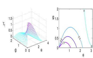
Figure 1: (Color online) Berry phase corresponding to the instantaneous eigenstate $|\Psi_{1}\rangle$ versus the rescaled coupling constant $g$ and the azimuthal angle $\theta$[Arc]. The plot was presented in units of $\pi$ for the Berry phase. The right panel is a contour plot for the left one.

From Fig.1 we see that the Berry phase is a monotonic function of the rescaled coupling constant, while it is maximized for intermediate values of the azimuthal angle $\theta$. The berry phase for the eigenstate 2 has a similar appearance as Fig.2 shows.

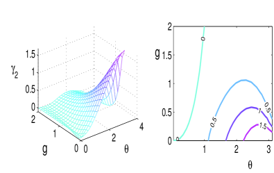
Figure 2: (Color online) The same as Figure 1, but for instantaneous eigenstate $|\Psi_{2}\rangle$

It is worth noting that $\gamma_{1}(\theta)=\gamma_{2}(\pi-\theta)$, this can be easily found by comparing the contour plots presented in Fig. 1 and 2. This symmetry originate from the Hamiltonian and it is clear that the eigenstate $|\Psi_{1}\rangle(|\Psi_{3}\rangle)$ is alternated with $|\Psi_{2}\rangle(|\Psi_{4}\rangle)$ when $\theta\ \leftrightarrow(\pi-\theta)$, this leads to the symmetry in the Berry phase. The contour plots presented in Fig.3 and 4 show the same symmetry indeed.

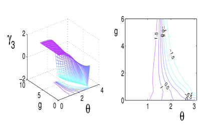
Figure 3: (Color online) Berry phase (in units of $\pi$) corresponding to the instantaneous eigenstate $|\Psi_{3}\rangle$ versus the rescaled coupling constant $g$ and the azimuthal angle $\theta$[Arc]. The right panel is a contour plot for the left one.

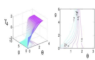
Figure 4: (Color online) The same as Figure 3, but for the instantaneous eigenstate $|\Psi_{4}\rangle$

Figure 5 shows the results of Berry phases corresponding to the four eigenstates Eq.(4) with a specific azimuthal angle $\theta=\theta_{0}=\frac{\pi}{4}$. With $g\rightarrow 0$ the Berry phases approach two values( in units of $\pi$) of $\gamma_{\pm}=(1\pm\cos\theta_{0})\simeq 1\pm 0.707$ as expected, whereas they approach zero with $g\rightarrow\infty$.

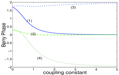
Figure 5: (Color online) The Berry phase vs. the rescaled coupling constant $g$ with a specific azimuthal angle $\theta=\frac{\pi}{4}$. The indices on the line indicate the eigenstate by which we got the Berry phase.

Now we are in a position to study the Berry phase of the subsystem, and to show what is the relation between these phases. Generally speaking a state of subsystem is no longer a pure one, so we have to adopt the definition of geometric phase for a mixed state sjoqvist1 , that is $\phi_{g}=\arg\mbox{Tr}(\rho_{0}U(t))$ with $\rho_{0}$ denoting the initial density matrix and $U(t)$ the transport operator which should fulfill the parallel transport evolution condition. This definition is available when the system from which we want to get geometric phases undergoes an unitary evolution. For the subsystems with non-zero couplings, however, the evolution of each subsystem is not unitary in general. So, here we borrow the idea presented in ericsson to define the Berry phase for a mixed state. A non-unitary evolution of a quantal state may be conveniently modelled by attaching an ancilla to the system, in our case the ancilla can always be taken to be the other spin-$\frac{1}{2}$ system. The geometric phase corresponding to this non-unitary evolution is then defined as the geometric phase of the whole system (system+ ancilla) that evolves unitarily. For an adiabatic cyclic evolution, this gives rise to a definition of Berry phase for a mixed state $\rho(t)=\sum_{j}p_{j}|E_{j}(t)\rangle\langle E_{j}(t)|,$

$$\gamma=\sum_{j}p_{j}\gamma_{j},$$ (7)

where $\gamma_{j}=i\int_{0}^{T}dt\langle E_{j}(t)|\dot{E}_{j}(t)\rangle$. The Berry phase Eq.(7) for a mixed state is just an average of the individual Berry phases, weighted by their eigenvalues $p_{j}$. To be sure, what we have is consistent with known results, we check that this expression reduces to the standard Berry phase $\gamma=i\int_{0}^{T}dt\langle\psi(t)|\dot{\psi}(t)\rangle$ for a pure state $\rho(t)=|\psi(t)\rangle\langle\psi(t)|$. In our case, we have four density matrices of mixed state for each subsystem, they correspond to the four instantaneous eigenstates of the Hamiltonian, respectively. For example, $\rho_{1}^{j}(t)=\mbox{Tr}_{2}|\Psi_{j}(t)\rangle\langle\Psi_{j}(t)|$ represents the $j$-th density matrix for subsystem 1 among the four density matrices, where $\mbox{Tr}_{2}$ denotes a trace over subsystem 2. The Berry phase corresponding to this state $\rho_{1}^{j}(t)$ is then given by Eq.(7). Actually, the definition Eq.(7) can be derived by the idea of the so-called purifications as follows. We may construct a pure state

$$|\Phi(t)\rangle=\sum_{j}\sqrt{p_{j}}|E_{j}(t)\rangle_{1}\otimes|j\rangle_{a}$$

for subsystem 1 + ancilla (for subsystem 2+ ancilla, in the same manner) such that

$$\mbox{Tr}_{a}|\Psi(t)\rangle\langle\Psi(t)|=\sum_{j}p_{j}|E_{j}(t)\rangle\langle E_{j}(t)|=\rho_{1}(t),$$

where $\mbox{Tr}_{a}$ denotes a trace over the ancilla and $|E_{j}(t)\rangle$ represent instantaneous eigenstates of $\rho_{1}(t)$. Since the states of the ancilla remain unchanged during the evolution, the Berry phase of the subsystem 1 is then the Berry phase of the compound (subsystem+ancilla), this yields the definition Eq.(7).

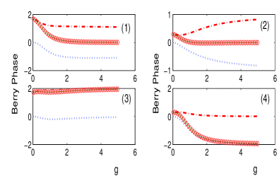
Figure 6: (Color online) The Berry phase for the composite system(diamond) and for subsystem 1(dash-dot) and subsystem 2 (dotted). A sum of the subsystem’s Berry phase is also presented in the figure(solid line, overlapped by the diamond line). The azimuthal angle $\theta=\frac{\pi}{4}$ was chosen for this plot.

The Berry Phase of the composite system and those of the two subsystems are illustrated in Fig.6, a sum of the subsystem’s Berry phase is also shown. There is an evidence that the Berry phase of the composite system can be decomposed into a sum of the subsystem’s Berry phases, it reveals the relation between geometric phases of entangled bipartite systems and those of their subsystems. We can prove this point indeed by expanding the instantaneous eigenstate of the composite system via Schmidt decomposition

$$|\Psi\rangle=\sum_{i}\sqrt{p_{i}}|e_{i}(t)\rangle_{1}\otimes|E_{i}(t)\rangle_{2},$$ (8)

where $|\Psi\rangle$ denotes one of the instantaneous eigenstates Eq. (4). This expansion yields the reduced density operator $\rho_{1}(t)=\sum_{i}p_{i}|e_{i}(t)\rangle\langle e_{i}(t)|$ and $\rho_{2}(t)=\sum_{i}p_{i}|E_{i}(t)\rangle\langle E_{i}(t)|$ for subsystems $1$ and $2$, respectively. By the definition Eq.  (3), the Berry phase corresponding to $|\Psi\rangle$ follows,

$$\gamma=i\int_{0}^{T}\sum_{j}p_{j}\langle e_{j}(t)|\dot{e}_{j}(t)\rangle dt+i\int_{0}^{T}\sum_{j}p_{j}\langle E_{j}(t)|\dot{E}_{j}(t)\rangle dt,$$ (9)

i.e., the Berry phase of the composite system adds up to be that of the composite system. This additivity holds mathematically when the Schmidt decomposition is available with time-independent coefficients $p_{i}$. Physically, time-independent coefficients $p_{i}$ indicate no population transfer among the eigenstates of the reduced density matrix of subsystem (this is what we called adiabaticity for the subsystem in this paper). Here the result that the Berry phase of the subsystem adds up to be that for the composite system remains unchanged for all two-subsystem compound when both the compound and the subsystems undergo a cyclic adiabatic evolution.

The observation of this prediction with NMR experiment is within the touch of current technology du . For instance, we can use Carbon-13 labelled chloroform in $d_{6}$ acetone as the sample, in which the single ${}^{13}C$ nucleus and the ${}^{1}H$ nucleus play the role of the two spin-$\frac{1}{2}$. The constant of spin-spin coupling $J\sigma_{1}^{z}\sigma_{2}^{z}$ in this case is $J\simeq(2\pi)214.5\mbox{Hz}$, and we may control the rescaled coupling constant $g$ by changing the magnitude of the external magnetic field. We would like to address that the interaction between the two spin-$\frac{1}{2}$ in our model is not a typical spin-spin coupling as that in NMR, but rather a toy model describing a double spin flip. So, we have to make a mapping when we employ the presentation in NMR system and when all subsystem are driven by the classical field. Finally, we want to discuss the problem of adiabaticity. Our study is based on an adiabatic cyclic evolution of the composite system. For any subsystem, however, the conditions of adiabaticity are not fulfilled in general, in this sense this is not a Berry phase but a geometric phase for a subsystem when the composite system itself is subject to an adiabatic evolution. But this is not the case in the Letter, it is easily to check that the eigenvalues of the reduced density matrix $\rho_{1}^{j}(t)=\mbox{Tr}_{2}(|\Psi_{j}(t)\rangle\langle\Psi_{j}(t)|$ (for any j) are independent of time, this indicate the population on the eigenstate of $\rho_{1}^{j}(t)$ remain unchanged note1 while the composite system follows an adiabatic evolution.

To sum up, we have theoretically investigated the Berry phase of a composite system and that of their subsystems. The Berry phase for a mixed state to our best knowledge is a concept new project. The relation between those phases is also presented and discussed, these results provide us a new way to control the Berry phase, we thus might find some applications in quantum computation. We are investigating possible applications of this effects and its connections to other quantum effects in different systems.

XXY acknowledges enlightening discussions with Dr Erik Sjöqvist and Dr Jiangfeng Du. This work is supported by EYTP of M.O.E, and NSF of China Project No. 10305002.

References

- (1) M. V. Berry, Proc. R. Soc. London A 392, 45(1984).
- (2) Geometric phase in physics, Edited by A. Shapere and F. Wilczek ( World Scientific, Singapore, 1989).
- (3) D. Thouless et al., Phys. Rev. Lett. 49, 405(1983); F. S. Ham, Phys. Rev. Lett. 58, 725 (1987); H. Mathur, Phys. Rev. Lett. 67,3325(1991);H. Svensmark and P. Dimon, Phys. Rev. Lett. 73, 3387(1994); M. Kitano and T. Yabuzaki, Phys. Lett. A 142, 321(1989).
- (4) C. P. Sun, Phys. Rev. D 41, 1318(1990).
- (5) Y. Aharonov and J. Anandan, Phys. Rev. Lett. 58,1593(1987); J. Samuel and R. Bhandari, Phys. Rev. Lett. 60, 2339(1988); N. Mukunda and R. Simon, Ann. Phys. (N.Y.) 205(1993); 269 (1993); A. K. Pati, Phys. Rev. A 52,2576(1995).
- (6) E. Sjöqvist et al., Phys. Rev. Lett. 85, 2845(2000);R. Bhandari, Phys. Rev. Lett. 89, 268901(2002); J. Anandan et al., Phys. Rev. Lett. 89, 268902(2002).
- (7) M. Ericsson et al., Phys. Rev. A 67,020101(R)(2003).
- (8) A. Carollo et al., Phys. Rev. Lett. 90,160402(2003); R. S. Whituey et al., Phys. Rev. Lett. 90, 190402(2003).
- (9) I. Fuentes-Guridi et al., Phys. Rev. Lett. 89, 220404 (2002).
- (10) E. Sjöqvist, Phys. Rev. A 62,022109(2000).
- (11) D. M. Tong, L. C. Kwek, and C. H. Oh, J. Phys. A 36, 1149(2003).
- (12) J. A. Jones, V. Vedral, A. Ekert, and G. Castagnoli, Nature(London) 403, 869(1999).
- (13) A. Ekert, M. Ericsson, P. Hayden, H. Inamori, J. A. Jones, K. K. L. Oi, and V. Vedral, J. Mod. Opt. 47, 2051(2000).
- (14) G. Falci, R. Fazio, G. M. Palma, J. Siewert, and V. Vedral, Nature(London)407, 355(2000).
- (15) X. B. Wang et al., Phys. Rev. Lett. 87, 097901 (2001).
- (16) J. Du et al., Phys. Rev. Lett. 91, 100403 (2003).
- (17) D. M. Tong, et al., Phys. Rev. A 68, 022106(2003).
- (18) The eigenstates of change with time, just as those of the composite system do.