Qubit Assisted Probing of Coherence Between States of a Macroscopic Apparatus

Abstract

I present a general scheme through which the evidence of a superposition involving distinct classical-like states of a macroscopic system can be probed. The scheme relies on a qubit being coupled to a macroscopic harmonic oscillator in such a way that it can be used to both prepare and probe a macroscopic superposition. Two potentially realizable implementations, one with a flux qubit coupled to a LC circuit, and the other with an ion-trap qubit coupled to the collective motion of several ions, are proposed.

Superpositions between distinct states of microscopic systems have been observed in several experiments. Macroscopic systems, on the other hand, are almost always found to be in states which are close approximations to classical points in phase space pointer1 . Due to environmental effects zurekpt ; caldeira , it is very hard to observe evidences of superpositions between such classical states of a macroscopic system (a system with a large value of mass or equivalent). Despite this, there has been a steady progress in schemes for observing quantum superpositions between classical states of macroscopic systems leggett ; zeilinger ; josexpt ; bose ; blencowe ; mancini ; simon . Some of these are actual experiments zeilinger ; josexpt or strongly aimed towards actual experiments blencowe ; simon . In this letter, I will present a generic scheme in which any qubit (assumed to remain coherent during the duration of the scheme), when coupled appropriately to a macroscopic (material or non-material) harmonic oscillator, can be used to both create and probe superpositions of states of the qubit-oscillator system which involve distinct classical states of the oscillator. This presents a mathematically unified setting for some earlier proposals (bose ; blencowe ). Furthermore, it helps to suggest a variety of schemes using specific qubit-harmonic oscillator combinations. I will illustrate this diversity of the scheme by presenting two potential implementations distinct from those proposed before bose ; blencowe .

There are models of decoherence of a superposition of states of macroscopic oscillator zurekpt ; caldeira ; venugopalan , which give decoherence rates in terms of macroscopic variables such as the mass $m$, dissipation constant $\gamma$ and frequency $\omega$ of the oscillator and temperature $\theta$ of the oscillator and its environment. The domain of validity of such simplistic (thermodynamically flavored) models, remain to be fully tested. For a superposition of two coherent states of the oscillator separated by a distance $\Delta x$ these models give the following heuristic formula for the decoherence time-scale

$$\tau_{D}=\hbar^{2}/\{D(\Delta x)^{2}\}$$ (1)

with $D=2m\gamma\hbar\omega(\bar{n}+\frac{1}{2})$ in which $\bar{n}=[\exp{(\hbar\omega/k_{B}\theta)}-1]^{-1}$ is the expected number of quanta in a harmonic oscillator. For $\theta=0$ we can rewrite $\tau_{D}=1/(2\gamma|\Delta\alpha|^{2})$ (where $\Delta\alpha$ is the amplitude difference of the superposed coherent states). This has been experimentally verified to hold exactly for a single trapped ion wineland . Our scheme, as I will show, can be used to test the same models for higher $\theta$ and larger $m$. This will extend the work of earlier decoherence experiments wineland ; haroche which have only tested the dependence of $\tau_{D}$ on $\Delta\alpha$ and $\gamma$, while leaving out the dependence on $m$ and $\theta$.

I will adopt the formula for the decoherence rate from a rigorous treatment of the measurement of a qubit by a harmonic oscillator venugopalan . In this sense, the current paper has a secondary objective of improving on earlier heuristic treatments of decoherence in the same setting bose . Moreover, the scheme presents a simple application of a single qubit. As large scale quantum computation is still somewhat distant, any use for a single qubit is currently of interest. The macroscopic harmonic oscillator can even be a system which usually acts as an apparatus for the qubit. Simply setting it to work in a regime different from that used in a typical measurement suffices to create the conditions of our experiment. In the rest of the paper, I will often refer to the harmonic oscillator as the apparatus.

Interference experiments are generally done by splitting the wave-function of a system, applying a relative phase between the two split components and subsequently interfering these components. For a macroscopic system, however, (1) coherent wave-function splitters are not readily available (notable exception being macro-molecules zeilinger ), (2) decoherence can be unacceptably large, and (3) the initial state is mixed (thermal). We describe below how to circumvent each problem. A natural way to avoid the absence of a wave-function splitter for a macroscopic system is to involve an auxiliary microscopic system (such as a qubit) and use it to both create and probe superpositions between distinct states of the combined microscopic and macroscopic system. I describe the general procedure in two steps. For convenient description, I will first assume that no environment interacts with either the qubit or the apparatus (I will incorporate such interactions in the next paragraph). In the first step, a coherent superposition $|\psi(0)\rangle_{Q}=(1/\sqrt{2})(|0\rangle_{Q}+|1\rangle_{Q})$ of the states of a qubit is prepared and a macroscopic system (which we call an apparatus) initially in a state $|\alpha\rangle_{A}$ (a close approximation to a classical point in phase space) is allowed to interact with it. The qubit-apparatus coupling is assumed to be such that in a time $t$ the following evolution takes place

$$|\psi(0)\rangle_{Q}|\alpha\rangle_{A}\rightarrow(1/\sqrt{2})(|0\rangle_{Q}|\alpha_{0}\rangle_{A}+|1\rangle_{Q}|\alpha_{1}\rangle_{A}).$$ (2)

We assume that states $|\alpha_{0}\rangle_{A}$ and $|\alpha_{1}\rangle_{A}$ are each close approximations to points in classical phase space with coordinates being uniquely determined by $\alpha_{0}$ and $\alpha_{1}$ respectively ($\alpha_{0}\neq\alpha_{1}$). Now an external field is applied to the apparatus to evolve the state in the right hand side of Eq.(2) to $\frac{1}{\sqrt{2}}(|0\rangle_{Q}|\alpha_{0}\rangle_{A}+e^{i\phi_{01}}|1\rangle_{Q}|\alpha_{1}\rangle_{A})$. It is ensured that the appearance of the relative phase $\phi_{01}$ is correlated to the presence of different apparatus states $|\alpha_{0}\rangle_{A}$ and $|\alpha_{1}\rangle_{A}$ in each component of the above superposition. Detection of $\phi_{01}$ is then the evidence of coherence between the states $|0\rangle_{Q}|\alpha_{0}\rangle_{A}$ and $|1\rangle_{Q}|\alpha_{1}\rangle_{A}$ after the first step. To detect this phase, we take the second step in which the qubit and apparatus are allowed to interact for another time interval $t$ such that

$$\frac{|0\rangle_{Q}|\alpha_{0}\rangle_{A}+e^{i\phi_{01}}|1\rangle_{Q}|\alpha_{1}\rangle_{A}}{\sqrt{2}}\rightarrow\frac{|0\rangle_{Q}+e^{i\phi_{01}}|1\rangle_{Q}}{\sqrt{2}}|\alpha\rangle_{A}.$$ (3)

In the above evolution, the apparatus is brought back to its original state and the relative phase between the superposed components of the joint system has become a relative phase between the states $|0\rangle_{Q}$ and $|1\rangle_{Q}$ of the qubit. The experiment is now concluded by determining the relative phase $\phi_{01}$ through a measurement of the state of the qubit only. (the same technique has been used for a trapped ion in Ref.wineland ).

For a macroscopic apparatus, there will also be decoherence during the evolution of $|\alpha\rangle_{A}$ to $|\alpha_{0}\rangle_{A}$ and $|\alpha_{1}\rangle_{A}$ and back. We will assume that only the states of the macroscopic apparatus decohere, but the states of the qubit do not (at least over the time-scale of our experiment). If the apparatus is under-damped (i.e., it loses hardly any energy during the experiment), the evolution in step one is modified to

$$|\psi(0)\rangle\langle\psi(0)|_{Q}|\alpha\rangle\langle\alpha|_{A}\rightarrow(1/2)(|0\rangle\langle 0|_{Q}|\alpha_{0}\rangle\langle\alpha_{0}|_{A}$$ (4)

$$+ |1\rangle\langle 1|_{Q}|\alpha_{1}\rangle\langle\alpha_{1}|_{A})+(e^{-{\cal D}_{01}}/2)(|0\rangle\langle 1|_{Q}|\alpha_{0}\rangle\langle\alpha_{1}|_{A}$$

$$+ |1\rangle\langle 0|_{Q}|\alpha_{1}\rangle\langle\alpha_{0}|_{A}),$$

where $e^{-{\cal D}_{01}}$ is the decoherence term (${\cal D}_{01}>0$). Note that in Eq.(4), the appearance of the decoherence term is in one to one correspondence with the appearance of terms $|0\rangle\langle 1|_{Q}|\alpha_{0}\rangle\langle\alpha_{1}|_{A}$ and $|1\rangle\langle 0|_{Q}|\alpha_{1}\rangle\langle\alpha_{0}|_{A}$. Thus a measurement of this term suffices to demonstrate the partial coherence (as quantified by $e^{-{\cal D}_{01}}$) between $|0\rangle_{Q}|\alpha_{0}\rangle_{A}$ and $|1\rangle_{Q}|\alpha_{1}\rangle_{A}$ after step one. We can thus dispense with the application of the relative phase $\phi_{01}$ ($e^{-{\cal D}_{01}}$ can itself be thought as arising from random relative phases) and directly proceed to step two, in which the modified evolution is

$$(1/2)(|0\rangle\langle 0|_{Q}|\alpha_{0}\rangle\langle\alpha_{0}|+|1\rangle\langle 1|_{Q}|\alpha_{1}\rangle\langle\alpha_{1}|_{A})$$ (5)

$$+ (e^{-{\cal D}_{01}}/2)(|0\rangle\langle 1|_{Q}|\alpha_{0}\rangle\langle\alpha_{1}|_{A}$$

$$+ |1\rangle\langle 0|_{Q}|\alpha_{1}\rangle\langle\alpha_{0}|_{A})\rightarrow(1/2)(|0\rangle\langle 0|_{Q}+|1\rangle\langle 1|_{Q})$$

$$+ (e^{-{\cal D}_{01}}/2)(|0\rangle\langle 1|_{Q}+|1\rangle\langle 0|_{Q})|\alpha\rangle\langle\alpha|_{A}.$$

In the above, equal decoherence factors have been assumed in both the steps. After the second step, the state of the qubit is measured to determine ${\cal D}_{01}$ and thereby the degree of coherence between $|0\rangle_{Q}|\alpha_{0}\rangle_{A}$ and $|1\rangle_{Q}|\alpha_{1}\rangle_{A}$ after step one. One of the problems with a macroscopic apparatus is that ${\cal D}_{01}$ can be so large that the measured degree of coherence is too small. However, in most reasonable models of decoherence, ${\cal D}_{01}$ also depends on the absolute value of the difference $\alpha_{0}-\alpha_{1}$ and can thereby be reduced by making this difference small. So no matter how macroscopic the apparatus is, we can always bring ${\cal D}_{01}\sim 1$, so that some coherence between $|0\rangle_{Q}|\alpha_{0}\rangle_{A}$ and $|1\rangle_{Q}|\alpha_{1}\rangle_{A}$ persists. Measuring ${\cal D}_{01}$ not only provides evidence of the partially coherent superposition between $|0\rangle_{Q}|\alpha_{0}\rangle_{A}$ and $|1\rangle_{Q}|\alpha_{1}\rangle_{A}$, but also allows us to systematically test the models of decoherence of the macroscopic apparatus.

A third problem associated with an interference experiment with a macroscopic system is its initial thermal state. For this, it is necessary to assume that irrespective of the initial state $|\alpha\rangle_{A}$, the same $\alpha_{1}-\alpha_{0}$ (i.e., the same ${\cal D}_{01}$) results. Moreover, we need to assume that the macroscopic system is a harmonic oscillator with $|\alpha\rangle_{A}$ being coherent states. Then any thermal state can be written as $\int p(\alpha)|\alpha\rangle\langle\alpha|_{A}d^{2}\alpha$, where $p(\alpha)$ are probabilities, which is a mixture of coherent states $|\alpha\rangle_{A}$. For each component $|\alpha\rangle\langle\alpha|_{A}$ of the mixture, the dynamics described in Eqs.(4) and (5) would hold, and if we measure the state of the qubit after the third step, we would measure the same decoherence factor $e^{-2{\cal D}_{01}}$ and thereby the degree of coherence between $|0\rangle_{Q}|\alpha_{0}\rangle_{A}$ and $|1\rangle_{Q}|\alpha_{1}\rangle_{A}$ at the end of the first step.

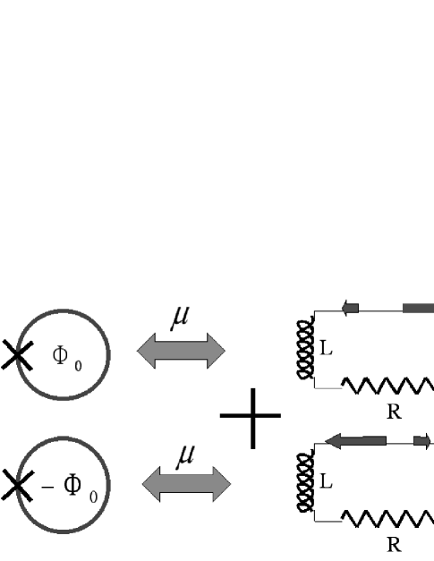
Figure 1: The figure shows the probing of macroscopic coherence by coupling a flux qubit to a macroscopic LC tank circuit. Being initially prepared in the state $(1/\sqrt{2})(|0\rangle_{Q}+|1\rangle_{Q})$, the flux qubit induces different flux values (current directions) in the circuit corresponding to its different flux states; the resulting macroscopic superposition is shown in the figure.

We will now propose a scheme using an explicit Hamiltonian for the qubit-apparatus-environment system, in which the apparatus is modeled as a harmonic oscillator. The first and the second steps will now be two successive parts of the same time evolution. We will use a model studied by Venugopalan venugopalan in the context of a quantum measurement (although, we will use it in a parameter regime different from that of a measurement). The Hamiltonian for the model can be written as

$$H=H_{Q}+H_{A}+H_{QA}+H_{AE},$$ (6)

where $H_{Q}$ is the qubit Hamiltonian, $H_{QA}$ is the qubit-apparatus interaction, $H_{A}$ is the apparatus Hamiltonian and $H_{AE}$ is the apparatus-environment interaction. These terms are explicitly given by

$$H_{A}=\frac{p^{2}}{2m}+\frac{1}{2}m\omega^{2}x^{2},~{}H_{Q}=\lambda\sigma_{Z},~{}H_{QA}=\epsilon x\sigma_{Z}$$ (7)

$$H_{AE}=\sum_{j}\frac{P_{j}^{2}}{2M_{j}}+\frac{M_{j}\Omega_{j}^{2}}{2}\bigl{(}X_{j}-\frac{C_{j}x}{M_{j}\Omega_{j}^{2}}\bigr{)}^{2}.$$ (8)

Here $x$ and $p$ denote the position and momentum of the harmonic oscillator (apparatus), $\lambda\sigma_{Z}$ is the the Hamiltonian of the qubit (for simplicity, we will set $\lambda=0$ for the rest of the paper; this does not affect our conclusions), and $\epsilon$ is the strength of the qubit-apparatus coupling. The last term represents the Hamiltonian for the environment (a bath of oscillators) and the apparatus-environment interaction. $X_{j}$ and $P_{j}$ are the position and momentum coordinates of the jth harmonic oscillator of the bath, $C_{j}$’s are the coupling strengths and $\Omega_{j}$s are the frequencies of the oscillators comprising the bath venugopalan .

Venugopalan venugopalan has found the complete solutions to the model for all parameter domains of the Hamiltonian given by Eqs.(6) and (8) in the Markovian limit ($k_{B}\theta<<\hbar\Omega_{\mbox{cut}}$ where $k_{B}=$ Boltzmann constant, $\hbar=$ Plank constant and $\Omega_{\mbox{cut}}=$ cutoff frequency of the environmental oscillators). Subsequently, Venugopalan has used the solutions only in the case of an overdamped oscillator ($\omega<<\gamma$ where where $\gamma$ is the relaxation rate of the oscillator) in the long time ($t\rightarrow\infty$) limit to analyze a measurement of the qubit’s state by the oscillator. Our aim here is to investigate coherence between distinct states of the oscillator and not to complete a measurement (in course of which, all coherence will be lost). Hence we concentrate on the under-damped regime of parameters of the oscillator ($\gamma<<\omega$) for times $t\leq T=2\pi/\omega$ (i.e., $T$ is one oscillation period of the oscillator). In this parameter domain, if the oscillator starts in an initial coherent state ($\rho_{A}(0)=|\alpha\rangle\langle\alpha|_{A}$) and the qubit in the state $(1/\sqrt{2})(|0\rangle_{Q}+|1\rangle_{Q})$ then the evolution of the system from $t=0$ to $t=T/2$ is taken to be step one of our protocol. At the end of this step the state is given by

$$\rho_{QA}(T/2)=\frac{1}{2}(|0\rangle\langle 0|_{Q}|\alpha_{0}\rangle\langle\alpha_{0}|_{A}+|1\rangle\langle 1|_{Q}|\alpha_{1}\rangle\langle\alpha_{1}|_{A})$$

$$+ \frac{e^{-{\cal D}_{01}}}{2}(e^{-i\phi_{01}}|0\rangle\langle 1|_{Q}|\alpha_{0}^{{}^{\prime}}\rangle\langle\alpha_{1}^{{}^{\prime}}|_{A}+e^{i\phi_{01}}|1\rangle\langle 0|_{Q}|\alpha_{1}^{{}^{\prime}}\rangle\langle\alpha_{0}^{{}^{\prime}}|_{A})$$

where $|\alpha_{j}\rangle_{A}$ and $|\alpha_{j}^{{}^{\prime}}\rangle_{A}$ (with $j=0,1$) are coherent states of the apparatus with

$$\alpha_{j}=-\alpha+(-1)^{j}\Delta x/2\delta_{x},~{}\alpha_{j}^{{}^{\prime}}=\alpha_{j}+i\Delta p/2\delta_{p}.$$ (10)

where $\delta_{x}=\sqrt{\hbar/2m\omega}$ and $\delta_{p}=\sqrt{m\hbar\omega/2}$ are the coherent state position and momentum spreads, $\Delta x=2\epsilon/m\omega^{2}$ is the separation between the coherent states $|\alpha_{0}\rangle_{A}$ and $|\alpha_{1}\rangle_{A}$,$\Delta p=D\Delta x/2\omega\hbar^{2}$ is an unwanted momentum shift, ${\cal D}_{01}=\frac{D(\Delta x)^{2}}{\hbar^{2}}\frac{T}{2}$ is the decoherence exponent and $\phi_{01}=-4\pi{\cal D}_{01}$. If we define a scaled dimensionless qubit-apparatus coupling strength $\chi$ as $\epsilon\delta_{x}/\hbar\omega$ and the quality factor $Q$ of the oscillator as $Q=\omega/\gamma$, then (in the high temperature $\bar{n}\approx k\theta/\hbar\omega>>1$ limit) we can rewrite the orders of magnitudes of the earlier quantities as

$$\frac{\Delta x}{2\delta_{x}}\sim\chi,~{}\frac{\Delta p}{2\delta_{p}}\sim\frac{\chi\bar{n}}{Q},~{}{\cal D}_{01}\sim\frac{\chi^{2}\bar{n}}{Q}.$$ (11)

We want Eq.(LABEL:statepi) to correspond to the state in the right hand side of Eq.(4) (apart from the unimportant phase factor $\phi_{01}$) and thus require $\alpha_{j}\approx\alpha_{j}^{{}^{\prime}}$, which in turn implies $\exp{[-\{\frac{\Delta p}{2\delta_{p}}\}^{2}]}=\exp{[-\{\frac{\chi\bar{n}}{Q}\}^{2}]}\approx 1$. This is clearly satisfied if we choose our parameters such that

$$Q^{2}>>(\chi\bar{n})^{2}.$$ (12)

We would also want (ideally) $\Delta x$ to be larger than or comparable to a coherent state width. This implies

$$\chi\geq 1.$$ (13)

Moreover, we want some coherence to be present between $|0\rangle_{Q}|\alpha_{0}\rangle_{A}$ and $|1\rangle_{Q}|\alpha_{1}\rangle_{A}$ in $\rho_{QA}(T/2)$. We thus want ${\cal D}_{01}\sim 1$ which implies

$$Q\sim\chi^{2}\bar{n}.$$ (14)

When the qubit-apparatus system is allowed to evolve further from $t=T/2$ to $t=T$ (this is the step two of our protocol), the final state is given by

$$\rho_{QA}(T) = (1/2)\{|0\rangle\langle 0|_{Q}+|1\rangle\langle 1|_{Q}$$ (15)

$$+ e^{-2{\cal D}_{01}}(|0\rangle\langle 1|_{Q}+|1\rangle\langle 0|_{Q})\}\otimes|\alpha\rangle\langle\alpha|_{A}.$$

Detecting the decoherence factor $e^{-2{\cal D}_{01}}$ by measuring the state of the qubit now corresponds to measuring a signature of the partial coherence between $|0\rangle_{Q}|\alpha_{0}\rangle_{A}$ and $|1\rangle_{Q}|\alpha_{1}\rangle_{A}$ at $t=T/2$.

A further aim of our scheme is to test the dependence of ${\cal D}_{01}$ on $\theta$ and $m$. From the expression of ${\cal D}_{01}$ in Eq.(11), and $\bar{n}\propto\theta$, it follows that ${\cal D}_{01}$ will vary in direct proportion with $\theta$. The dependence on $m$ is trickier to test. One has to create the same $\Delta x$ for different $m$ to make a fair study of the dependence of ${\cal D}_{01}$ with $m$. As Eq.(11) suggests, ${\cal D}_{01}\propto\chi^{2}\sim(\Delta x)^{2}/4\delta_{x}^{2}\propto m(\Delta x)^{2}$. Thus if one creates the same $\Delta x$ for different $m$, then ${\cal D}_{01}$ should be found to be directly proportion to $m$.

We now proceed to suggest some potentially realizable experiments in which the above scheme can be tested. In the first realization, we take the qubit to be a flux qubit Makhlin coupled by a flux-flux coupling to a LC tank circuit prance , which is the macroscopic harmonic oscillator (apparatus) as shown in Fig.1. The $|0\rangle_{Q}$ and $|1\rangle_{Q}$ states of the qubit correspond to flux values $\pm\Phi_{0}$ with $\Phi_{0}=\hbar/2e$ (where $e$ is electronic charge). The flux variable of the qubit can thus be written as the operator $\Phi_{0}\sigma_{z}$. For the qubit-circuit coupled system everitt

$$H_{A}=(C/2)\dot{\Phi}^{2}+(1/2L)\Phi^{2},~{}H_{QA}=\mu\Phi(\Phi_{0}\sigma_{z})/\Lambda$$ (16)

where $C$ and $L$ are the capacitance and the inductance of the circuit, $\Phi$ is the flux through the circuit, $\Lambda$ is the inductance of the qubit, $\mu$ is a dimensionless coupling (flux linkage) between the qubit and the circuit. From Eqs.(16) it is evident that $\Phi$ and $C$ are the electrical counterparts of $x$ and $m$ respectively. For this system, $\epsilon=\mu\Phi_{0}/\Lambda,~{}\gamma=R/2L,~{}\omega=1/\sqrt{LC}$.

We now make an explicit choice of parameters of the qubit and the circuit to show that the three conditions for our experiment can be satisfied. We choose $\Lambda\sim 100$pH Makhlin for the flux qubit. For the circuit, we choose $L=\sim 100$$\mu$H, $C\sim 100$pF (a macroscopic value in comparison to the available $fF$ capacitances Makhlin ), $R\sim 1\Omega$. This gives $Q\sim 10^{3}$ at $\omega\sim 10$MHz ($Q\sim 10^{6}$ for $\omega\sim 10$KHz grav to $Q\sim 10^{2}$ for $\omega\sim 1$GHz cmos are achievable). We assume the temperature of the circuit and its environment to be $\theta\sim 10$mK (same as that of the flux qubit Makhlin ). With this choice, $\bar{n}\sim 100$ and

$$Q^{2}/\bar{n}^{2}\sim 10^{2},$$ (17)

thereby satisfying Eq.(12). We choose $\mu\sim 10^{-6}$ to have

$$\chi\sim\sqrt{10},~{}\chi^{2}\bar{n}\sim 10^{3}\sim Q$$ (18)

which implies that Eqs.(13) and (14) are satisfied.

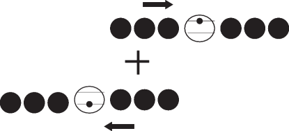
Figure 2: The figure shows the probing of macroscopic coherence by coupling the internal levels of a single ion to the collective motional state of several ions in a trap. Being initially prepared in the state $(1/\sqrt{2})(|0\rangle_{Q}+|1\rangle_{Q})$, the internal level qubit displaces the collective motional state differently corresponding to its two states; the resulting macroscopic superposition is shown in the figure.

Next we propose a different physical realization using a linear ion trap wineland . In this case, we use the internal levels of a single trapped ion as the qubit and the collective motion of $N$ ions (with large $N$) as the macroscopic oscillator as shown in Fig.2. The qubit-apparatus coupling term of the Hamiltonian for the system is wineland3

$$H_{QA}=(\hbar g\eta_{0}/\sqrt{N}\delta_{x})x\sigma_{z},$$ (19)

where $g$ is the vacuum Rabi frequency and $\eta_{0}$ is the Lamb-Dicke parameter for a single ion. We assume $N\sim 100$, $\omega\sim 1$MHz (an order less than in blatt ), $g\sim 100\sqrt{10}$MHz (300 times higher than in wineland4 ) and $\eta_{0}\sim 0.1\sqrt{10}$ (nearly same as in wineland4 ). With these choices

$$\chi\sim g\eta_{0}/\sqrt{N}\omega\sim 10,$$ (20)

which satisfies Eq.(13). We now choose $\theta\sim 0.1$mK, so that $\bar{n}\sim 10$. We also note that for the natural (ambient) reservior $\gamma\sim 1$KHz wineland4 , which implies a quality factor $Q\sim 10^{3}$. This implies

$$(Q/\chi\bar{n})^{2}\sim 10^{2},~{}\bar{n}\chi^{2}/Q\sim 1,$$ (21)

which satisfies Eq.(12) and Eq.(14).

In this paper, I have presented a general scheme for probing evidences of superpositions which involve distinct classical-like states of a macroscopic object. Though realizations with two specific qubit-harmonic oscillator combinations are proposed, the paper opens up the scope for applying to any other combination. It also provides a unified mathematical setting for some earlier proposals bose ; blencowe and can be used to probe the dependence of decoherence rate on the mass and temperature. In comparison to the schemes used in decoherence experiments so far haroche ; wineland , this is more easily extendable to macroscopic oscillators where it might be difficult to switch qubit-oscillator interactions on and off (such as the radiation pressure interaction bose ; mancini ) and where the superposition itself forms over such a length of time that decoherence during the formation is important.

This work is supported by the NSF under Grant Number EIA-00860368. I thank P. Delsing for valuable comments.

References

- (1) W. H. Zurek, S. Habib and J. P. Paz, Phys. Rev. Lett. 70, 1187 (1993).
- (2) W. H. Zurek, Physics Today 44 (10), 36 (1991).
- (3) A. O. Caldeira and A. J. Leggett, Physica A 121, 587 (1983).
- (4) A. J. Leggett and A. Garg, Phys. Rev. Lett. 54, 857 (1985).
- (5) M. Arndt et. al., Nature 401, 680 (1999).
- (6) J. Friedman et. al. Nature 406 43 (2000); C. H. van der Wall et. al Science 290 773 (2000).
- (7) S. Bose, K. Jacobs and P. L. Knight, Phys. Rev. A 59, 3204 (1999).
- (8) A. D. Armour, M. P. Blencowe and K. C. Schwab, Phys. Rev. lett 88, 148301 (2002).
- (9) S. Mancini, V. Giovannetti, D. Vitali, and P. Tombesi, Phys. Rev. Lett. 88, 120401 (2002).
- (10) W. Marshall, C. Simon, R. Penrose and D. Bouwmeester, quant-ph/0210001 (2002).
- (11) A. Venugopalan, Phys. Rev. A 61, 012102 (1999).
- (12) C. J. Myatt et. al., Nature 403, 269 (2000).
- (13) M. Brune et. al., Phys. Rev. Lett. 77 4887 (1996).
- (14) Y. Makhlin, G. Schön and A. Shnirman, Rev. Mod. Phys. 73, 357 (2001).
- (15) R. J. Prance et. al., Phys. Rev. Lett. 82, 5401 (1999).
- (16) M. J. Everitt et. al., Phys. Rev. B 63, 144530 (2001).
- (17) M. Bonaldi et. al., Rev. of Sci. Inst. 70, 1851 (1999).
- (18) P. Kinget and R. Frye, Proc. of the ESSCIRC, pp. 364-367 (1998).
- (19) D. J. Wineland et. al., J. Res. Natl. Inst. Stand. Technol. 103, 259 (1998).
- (20) F. Schmidt-Kaler et. al.,Nature 422 (2003).
- (21) C. Monroe et. al., Science 272, 1131 (1996).