Quantum-state extraction from high-$\bm{Q}$ cavities

Abstract

The problem of extraction of a single-mode quantum state from a high-$Q$ cavity is studied for the case in which the time of preparation of the quantum state of the cavity mode is short compared with its decay time. The temporal evolution of the quantum state of the field escaping from the cavity is calculated in terms of phase-space functions. A general condition is derived under which the quantum state of the pulse built up outside the cavity is a nearly perfect copy of the quantum state the cavity field was initially prepared in. The results show that unwanted losses prevent the realization of a nearly perfect extraction of nonclassical quantum states from high-$Q$ optical microcavities with presently available technology.

I Introduction

High-$Q$ cavity QED has offered a number of novel possibilities of quantum-state engineering (see, e.g, Refs. Raimond01 ; Pinkse00 ; Hood00 ; Doherty00 and references therein). In particular, it provides promising tools to generate nonclassical quantum states of atoms and light for further use. Accordingly various applications have been proposed, with special emphasis on quantum communication and computation Knill01 ; Enk98 ; Tregenna02 . In contrast to atomic states, the usage of quantum states of light as carriers of quantum information is especially appropriate, due to the reliability of light to propagate over long distances Pan03 ; Bennett00 .

Various schemes for generating nonclassical light in cavities have been considered. They are typically based on effective two-level atoms. A generator of single photon Fock states in an active microcavity with pump self-regularization has been presented Martini96 . It has also been shown experimentally that an entangled state of two nondegenerate cavity modes can be produced with means of a sequence of differently tuned interactions of a pair of single atoms with the two cavity modes Rauschenbeutel01 , and a scheme for entangling two modes of spatially separated cavities by consecutively passing through them atoms has been purposed Browne03 . A scheme has been proposed Domokos98 and experimentally realized Brattke01 for the generation of photon number states on demand, by subjecting single two-level atoms passing through a cavity to $\pi$ pulse interaction. Similarly, a proposal has been made for entangling two cavity modes via interaction with a bunch of two-level atoms assisted by a strong classical driving field Solano03 . Schemes that exploit multilevel atoms have also been studied both theoretically Parkins95 ; Lange00 and experimentally Hennrich00 , with special emphasis on effective three-level atoms of $\Lambda$ type.

The main obstacles to generate nonclassical states are the various decoherence effects associated with, e.g., the motion and spontaneous emission of the atoms as well as scattering, absorption, and transmission of the photon field. Several proposals have been made to reduce the effect of decoherence due to the atomic motion Duan03 . In order to reduce unwanted spontaneous emission in schemes that exploit multi-level atoms, adiabatic transfer techniques have been promising Parkins95 ; Hennrich00 ; Lange00 . Moreover, the adiabatic passage is the main idea of the proposal of quantum networks of trapped atoms, where cavity modes provide communication channels, by leaking out of the cavities and propagating via optical interconnectors Cirac97 . Scattering and absorption losses, which are unavoidably connected with any material system, may be reduced by well designed cavities and the use of materials showing extremely weak absorption, and almost perfectly reflecting mirrors reduce the transmission losses. In particular, in Ref. Zippilli03 a method is presented for the protection of a generic quantum state of a cavity mode against the decohering effects of photon losses by feedback atoms crossing the cavity mode.

On the other hand, transmission losses are necessarily required to be taken into account in order to implement high-$Q$ cavities that can serve as sources that emit nonclassical radiation for further use outside the cavities Hennrich00 ; Kuhn02 ; Rempe92 ; Hood01 ; Pelton02 . The natural question arises whether or not nonclassical states of light, once generated inside a high-$Q$ cavity, can be extracted from the cavity and what the ultimate limits are. In the schemes considered, it is often made the ad hoc assumption of nearly perfect extraction (see, e.g., Refs. Martini96 ; Lange00 ; Saavedra00 ; Cirac97 ). The fact however is that even very small material absorption may be expected to lead to drastic quantum state degradation Scheel01 .

Recently, homodyne detection of the quantum state of the field leaving a high-$Q$ cavity has been studied theoretically Santos01 . From the results it might be expected that the quantum state, in which an excited cavity mode is prepared at some initial time, can be perfectly extracted from the cavity, so that after sufficiently long time, i.e., when the cavity is effectively empty, the pulse which has left the cavity is in the same quantum state as the cavity mode initially was. However, in the analysis the effects of unwanted losses (such as absorption and scattering losses) on the extracted quantum state have not been considered. Moreover, instead of calculating the quantum state of the outgoing field directly, the authors base the derivation on an operational definition of the Wigner function in terms of collective mode operators introduced within the frame of the homodyne detection scheme considered. The reason is that they claim that due to the mode continuum outside the cavity the Wigner function would be ill defined.

In this paper, we directly calculate as a function of time the quantum state of the pulse which leaves a high-$Q$ cavity and may be used for further processing. The calculations are performed for arbitrary $s$-parametrized phase space functions, including the Wigner function. Taking into account both transmission and unwanted losses of the cavity mode, we show that the crucial parameter for the efficiency of quantum state extraction is the ratio of absorption losses to transmission losses of the cavity mode. As we will see, a quantum state can be almost perfectly extracted after sufficiently long time, only if the value of this ratio is sufficiently small, thereby the truly required smallness sensitively depending on the nonclassical features of the state.

The outline of the paper is as follows. In Sec. II the model is explained and the basic equations, including the operator input-output relations, are given. The quantum state of the outgoing field is calculated in Sec. III, and Sec. IV presents two examples. Finally, a summary and some concluding remarks are given in Sec. V.

II Basic equations

II.1 Quantum Langevin equation

Let us consider a one-dimensional high-$Q$ cavity bounded with a perfectly reflecting mirror at $x$ $\!=$ $\!0$ and an almost perfectly reflecting mirror at $x$ $\!=$ $\!l$. For a high-$Q$ cavity, the widths $\gamma_{k}$ of the cavity modes at frequencies $\omega_{k}$ $\!=$ $\!k\pi c/l$ are very small compared with their separation $\Delta\omega$ $\!=$ $\!\omega_{k+1}$ $\!-$ $\!\omega_{k}$ $\!=$ $\!\pi c/l$, where $c$ is the velocity of light. Being interested in resolving times that are large compared with the time of propagation of light through the cavity, we may expand the intracavity field in terms of standing waves at frequencies $\omega_{k}$, where the associated photon creation and annihilation operators $\hat{a}_{k}^{\dagger}$ and $\hat{a}_{k}$, respectively, obey quantum Langevin equations Gardiner85 ; Knoell91 . For sufficiently large $Q$ values, we may further assume that the time of excitation and preparation of a cavity wave in a (desired) quantum state is short compared with its decay time (but still long compared with the propagation time through the cavity). In this case, the process of preparation of the cavity quantum state is well separated from the process of its transmission to the outside space.

Let $\hat{\varrho}_{\mathrm{cav}}$ be the quantum state an excited cavity wave is prepared in at some initial time $t_{0}$. For times $t$ $\!\geq$ $\!t_{0}$, the corresponding Langevin equation for the photon annihilation operator associated with the excited mode then reads

$$\dot{\hat{a}}=-i\left[\omega_{\mathrm{cav}}-{\textstyle\frac{i}{2}}\left(\gamma_{\mathrm{rad}}+\gamma_{\mathrm{abs}}\right)\right]\hat{a}$$ (1)

$$\hskip 8.61108pt+\left(\frac{c}{2l}\right)^{1/2}T\hat{b}_{\mathrm{in}}(t)+\left(\frac{c}{2l}\right)^{1/2}A\hat{c}(t).$$

In the first term,

$$\gamma_{\mathrm{rad}}=\frac{c}{2l}|T|^{2}$$ (2)

is the decay rate of the cavity mode which results from the transmission losses due to the radiative input-output coupling, and

$$\gamma_{\mathrm{abs}}=\frac{c}{2l}|A|^{2}$$ (3)

is the decay rate which results from the unwanted losses, briefly referred to as absorption losses in the rest of the paper, such as the unavoidably existing material absorption and scattering. For a high-$Q$ cavity, both the transmission coefficient $T$ and the absorption coefficient $A$ are very small compared with unity ($|T|$ $\!\ll$ $\!1$, $|A|$ $\!\ll$ $\!1$). Note that $T$ and $A$ are taken at the cavity-mode frequency $\omega_{\mathrm{cav}}$. The second term in Eq. (1) is the Langevin noise force arising from the input radiation field, where

$$\hat{b}_{\mathrm{in}}(t)=\frac{1}{\sqrt{2\pi}}\int_{\Delta\omega}\mbox{\rm d}\omega\,\hat{b}_{\mathrm{in}}(\omega,t)$$ (4)

$$=\frac{1}{\sqrt{2\pi}}\int_{\Delta\omega}\mbox{\rm d}\omega\,\hat{b}(\omega,t_{0})\,e^{-i\omega(t-t_{0})},$$

and the third term is the Langevin noise force associated with absorption, where

$$\hat{c}(t)=\frac{1}{\sqrt{2\pi}}\int_{\Delta\omega}\mbox{\rm d}\omega\,\hat{c}(\omega,t)$$ (5)

$$=\frac{1}{\sqrt{2\pi}}\int_{\Delta\omega}\mbox{\rm d}\omega\,\hat{c}(\omega,t_{0})\,e^{-i\omega(t-t_{0})}.$$

Here and in the following, the notation $\int_{\Delta\omega}\mbox{\rm d}\omega\ldots$ is used to indicate that the integration runs over frequencies in the interval $[\omega_{\mathrm{cav}}$ $\!-$ $\!\Delta\omega/2,\,\omega_{\mathrm{cav}}$ $\!+$ $\!\Delta\omega/2]$. The operators $\hat{a}(t)$, $\hat{b}(\omega,t)$, and $\hat{c}(\omega,t)$ satisfy the familiar bosonic equal-time commutation relations

$$\left[\hat{a}(t),\hat{a}^{\dagger}(t)\right]=1,$$ (6)

$$\bigl{[}\hat{b}_{\mathrm{in}}(\omega,t),\hat{b}_{\mathrm{in}}^{\dagger}(\omega^{\prime},t)\bigr{]}=\delta(\omega-\omega^{\prime}),$$ (7)

$$\left[\hat{c}(\omega,t),\hat{c}^{\dagger}(\omega^{\prime},t)\right]=\delta(\omega-\omega^{\prime}).$$ (8)

It is not difficult to see that the solution of Eq. (1) can be given in the form of

$$\hat{a}(t)\,=\,\hat{a}(t_{0})e^{-i\left[\omega_{\mathrm{cav}}-\frac{i}{2}({\gamma_{\mathrm{rad}}+\gamma_{\mathrm{abs}}})\right](t-t_{0})}$$ (9)

$$+\left(\frac{c}{2l}\right)^{1/2}\!T\!\int_{t_{0}}^{t}\mbox{\rm d}t^{\prime}\,e^{-i\left[\omega_{\mathrm{cav}}-\frac{i}{2}({\gamma_{\mathrm{rad}}+\gamma_{\mathrm{abs}}})\right](t-t^{\prime})}\hat{b}_{in}(t^{\prime})$$

$$+\left(\frac{c}{2l}\right)^{1/2}\!A\!\int_{t_{0}}^{t}\mbox{\rm d}t^{\prime}\,e^{-i\left[\omega_{\mathrm{cav}}-\frac{i}{2}(\gamma_{\mathrm{rad}}+\gamma_{\mathrm{abs}})\right](t-t^{\prime})}\hat{c}(t^{\prime}).\quad$$

II.2 Input-output relation

In close analogy to Eq. (4), output operators

$$\hat{b}_{\mathrm{out}}(t)=\frac{1}{\sqrt{2\pi}}\int_{\Delta\omega}\mbox{\rm d}\omega\,\hat{b}_{\mathrm{out}}(\omega,t)$$ (10)

$$=\frac{1}{\sqrt{2\pi}}\int_{\Delta\omega}\mbox{\rm d}\omega\,\hat{b}(\omega,t_{1})\,e^{-i\omega(t-t_{1})}\quad(t<t_{1})\quad$$

can be introduced, where, similar to Eq. (7), the bosonic commutation relation

$$\bigl{[}\hat{b}_{\mathrm{out}}(\omega,t),\hat{b}_{\mathrm{out}}^{\dagger}(\omega^{\prime},t)\bigr{]}=\delta(\omega-\omega^{\prime})$$ (11)

is valid. Taking into account that, on the time scale under consideration, the lower and upper integration limits of the frequency integrals can be extended, with little error, to $-\infty$ and $+\infty$, respectively, from Eqs. (4) and (10) together with the commutation relations (7) and (11) it then follows that the commutation relations

$$\bigl{[}\hat{b}_{\mathrm{in}}(t),\hat{b}_{\mathrm{in}}^{\dagger}(t^{\prime})\bigr{]}=\delta(t-t^{\prime})$$ (12)

and

$$\bigl{[}\hat{b}_{\mathrm{out}}(t),\hat{b}_{\mathrm{out}}^{\dagger}(t^{\prime})\bigr{]}=\delta(t-t^{\prime})$$ (13)

may be regarded as being valid. In a similar way, from Eqs. (5) and (8) we derive

$$\left[\hat{c}(t),\hat{c}^{\dagger}(t^{\prime})\right]=\delta(t-t^{\prime}).$$ (14)

Other important commutation rules are

$$\bigl{[}\hat{a}(t),\hat{b}_{\mathrm{in}}(t^{\prime})\bigr{]}=\bigl{[}\hat{a}^{\dagger}(t),\hat{b}_{\mathrm{in}}(t^{\prime})\bigr{]}=0\quad\mathrm{if}\quad t<t^{\prime}.$$ (15)

The output operator $\hat{b}_{\mathrm{out}}(t)$ can be related to the cavity operator $\hat{a}(t)$ and the input operator $\hat{b}_{\mathrm{in}}(t)$ according to the input-output relation

$$\hat{b}_{\mathrm{out}}(t)=\left(\frac{c}{2l}\right)^{1/2}T\hat{a}(t)+R\hat{b}_{\mathrm{in}}(t),$$ (16)

where

$$R=-\frac{T}{T^{*}}\,.$$ (17)

We renounce to repeat its derivation here, but refer the reader to the literature Gardiner85 ; Knoell91 . In Ref. Gardiner85 the derivation of Eq. (16) (with real $T$) is based on quantum noise theories whereas in Ref. Knoell91 a more rigorous QED derivation is given (also see Ref. Vogel94 ). Equation (16) corresponds to the following equation for the continuous-mode output operators $\hat{b}_{\mathrm{out}}(\omega,t)$:

$$\hat{b}_{\mathrm{out}}(\omega,t)$$ (18)

$$\,=\,\left(\frac{c}{2l}\right)^{1/2}T\lim_{t_{1}\rightarrow t_{+}}\,\frac{1}{\sqrt{2\pi}}\int_{t_{0}}^{t_{1}}\mbox{\rm d}t^{\prime}\,e^{-i\omega(t-t^{\prime})}\hat{a}(t^{\prime})$$

$$\hskip 8.61108pt+\,R\hat{b}(\omega,t_{0})\,e^{-i\omega(t-t_{0})}.\qquad$$

The proof of this equation is straightforward. Substituting Eq. (18) into Eq. (10), performing the frequency integral as before (i.e., extending the integration limits to $\mp\infty$), and recalling Eq. (4), we exactly arrive at Eq. (16). Note that $\hat{b}_{\mathrm{out}}(\omega,t)$ and $\hat{b}_{\mathrm{out}}^{\dagger}(\omega,t)$, as given by Eq. (18), fulfill the commutation rule (11).

We now substitute Eq. (9) together with Eqs. (4) and (5) into Eq. (18) to obtain

$$\hat{b}_{\mathrm{out}}(\omega,t)=F^{*}(\omega,t)\hat{a}(t_{0})+\hat{B}(\omega,t),$$ (19)

where the function $F(\omega,t)$ is defined by

$$F(\omega,t)=\frac{i}{\sqrt{2\pi}}\left(\frac{c}{2l}\right)^{1/2}T^{*}\,e^{i\omega(t-t_{0})}$$

$$\times\frac{\exp\left\{-i\left[\omega\!-\!\omega_{\mathrm{cav}}\!-\!\frac{i}{2}(\gamma_{\mathrm{rad}}\!+\!\gamma_{\mathrm{abs}})\right](t\!-\!t_{0})\right\}\!-\!1}{\omega-\omega_{\mathrm{cav}}-\frac{i}{2}(\gamma_{\mathrm{rad}}+\gamma_{\mathrm{abs}})}\,,$$

and the operator $\hat{B}(\omega,t)$ is a linear functional of the operators $\hat{b}(\omega,t_{0})$ and $\hat{c}(\omega,t_{0})$ according to

$$\hat{B}(\omega,t)=\int_{\Delta\omega}\mbox{\rm d}\omega^{\prime}G^{*}(\omega,\omega^{\prime},t)\hat{b}(\omega^{\prime},t_{0})$$ (21)

$$\hskip 30.1388pt+\int_{\Delta\omega}\mbox{\rm d}\omega^{\prime}H^{*}(\omega,\omega^{\prime},t)\hat{c}(\omega^{\prime},t_{0}).$$

Here, the functions $G(\omega,\omega^{\prime},t)$ and $H(\omega,\omega^{\prime},t)$, respectively, are defined by

$$G(\omega,\omega^{\prime},t)=T^{*}\xi(\omega,\omega^{\prime},t)+R^{*}e^{i\omega^{\prime}(t-t_{0})}\delta(\omega-\omega^{\prime})$$ (22)

and

$$H(\omega,\omega^{\prime},t)=A^{*}\xi(\omega,\omega^{\prime},t),$$ (23)

where $\xi(\omega,\omega^{\prime},t)$ reads

$$\xi(\omega,\omega^{\prime},t)=\frac{1}{2\pi}\frac{c}{2l}\,T^{*}\frac{1}{\omega-\omega_{\mathrm{cav}}-\frac{i}{2}(\gamma_{\mathrm{rad}}+\gamma_{\mathrm{abs}})}$$ (24)

$$\times\,\left\{\frac{e^{i\omega^{\prime}(t-t_{0})}-e^{i\left[\omega_{\mathrm{cav}}+\frac{i}{2}(\gamma_{\mathrm{rad}}+\gamma_{\mathrm{abs}})\right](t-t_{0})}}{\omega^{\prime}-\omega_{\mathrm{cav}}-\frac{i}{2}(\gamma_{\mathrm{rad}}+\gamma_{\mathrm{abs}})}\right.$$

$$\left.\qquad-\,\frac{e^{i\omega(t-t_{0})}-e^{i\omega^{\prime}(t-t_{0})}}{\omega-\omega^{\prime}}\right\}.\qquad\qquad$$

It is not difficult to see that from Eq. (19) together with the commutation rules (6) and (11) it follows that

$$\left[\hat{B}(\omega,t),\hat{B}^{\dagger}(\omega^{\prime},t)\right]=\delta(\omega-\omega^{\prime})-F^{*}(\omega,t)F(\omega^{\prime},t).$$ (25)

Note that

$$\bigl{[}\hat{a}(t_{0}),\hat{B}(\omega,t)\bigr{]}=\bigl{[}\hat{a}(t_{0}),\hat{B}^{\dagger}(\omega,t)\bigr{]}=0.$$ (26)

III Quantum state of the output field

III.1 Characteristic functional

To calculate the quantum state of the output field in the frequency interval $[\omega_{\mathrm{cav}}$ $\!-$ $\!\Delta\omega/2,\,\omega_{\mathrm{cav}}$ $\!+$ $\!\Delta\omega/2]$, we start from its characteristic functional

$$C_{\mathrm{out}}[\beta(\omega),t]$$ (27)

$$=\mathrm{Tr}\left\{\hat{\varrho}\,\exp\left[\int_{\Delta\omega}\!\mbox{\rm d}\omega\,\beta(\omega)\hat{b}^{\dagger}_{out}(\omega,t)-\mathrm{H.c.}\right]\right\},\quad$$

where $\hat{\varrho}$ is the density operator of the initial quantum state of the overall system, i.e., its quantum state at $t$ $\!=$ $\!t_{0}$. To further handle the functional, it is convenient to regard the integral as the limit of a sum, perform the calculations for the sum, and take the limit at the end of the calculations. That is to say, we write

$$C_{\mathrm{out}}[\beta(\omega),t]=\lim_{N\to\infty}C_{\mathrm{out}}(\bm{\beta},t)$$ (28)

[$\bm{\beta}$ $\!\equiv$ $\!(\beta_{1},\beta_{2},\ldots,\beta_{N})$], where

$$C_{\mathrm{out}}(\bm{\beta},t)=\mathrm{Tr}\left\{\hat{\varrho}\,\exp\!\left[\sum_{n=1}^{N}\beta_{n}\hat{b}^{\dagger}_{n}(t)-\mathrm{H.c.}\right]\right\}.$$ (29)

Here, $\beta_{n}$ and $\hat{b}_{n}(t)$, respectively, are defined by

$$\beta_{n}=\frac{1}{\sqrt{\delta\omega}}\int\limits_{\omega_{n}-\delta\omega/2}^{\omega_{n}+\delta\omega/2}\mbox{\rm d}\omega\,\beta(\omega)=\sqrt{\delta\omega}\,\beta(\omega_{n})$$ (30)

and

$$\hat{b}_{n}(t)=\frac{1}{\sqrt{\delta\omega}}\int\limits_{\omega_{n}-\delta\omega/2}^{\omega_{n}+\delta\omega/2}\mbox{\rm d}\omega\,\hat{b}_{\mathrm{out}}(\omega,t)$$ (31)

($\delta\omega$ $\!=$ $\!\Delta\omega/N$). Note that

$$\bigl{[}\hat{b}_{n}(t),\hat{b}_{n^{\prime}}^{\dagger}(t)\bigr{]}=\delta_{nn^{\prime}}\,.$$ (32)

The discrete version of Eq. (19) then reads

$$\hat{b}_{n}(t)=F^{*}_{n}(t)\hat{a}(t_{0})+\hat{B}_{n}(t)\,,$$ (33)

where $F_{n}(t)$ and $\hat{B}_{n}(t)$ being defined according to Eqs. (30) and (31), respectively, with $F(\omega,t)$ and $\hat{B}(\omega,t)$ instead of $\beta(\omega)$ and $\hat{b}_{\mathrm{out}}(\omega,t)$, respectively, and Eq. (25) changes to

$$\bigl{[}\hat{B}_{n}(t),\hat{B}_{n^{\prime}}^{\dagger}(t)\bigr{]}=\delta_{nn^{\prime}}-F_{n}^{*}(t)F_{n^{\prime}}(t).$$ (34)

Let us assume that the (initial) density operator $\hat{\varrho}$ is factorable as

$$\hat{\varrho}=\hat{\varrho}_{\mathrm{cav}}\otimes\hat{\varrho}_{\mathrm{in}}\otimes\hat{\varrho}_{\mathrm{abs}}$$ (35)

($\hat{\varrho}_{\mathrm{cav}}$, density operator of the cavity mode; $\hat{\varrho}_{\mathrm{in}}$, density operator of the input field; $\hat{\varrho}_{\mathrm{abs}}$, density operator of the dissipative system responsible for absorption). Substituting Eq. (33) into Eq. (29), we may write, on recalling Eq. (26),

$$C_{\mathrm{out}}(\bm{\beta},t)=\mathrm{Tr}\left\{\hat{\varrho}_{\mathrm{cav}}\exp\!\left[\sum_{n=1}^{N}\beta_{n}F_{n}(t)\hat{a}^{\dagger}(t_{0})-\mathrm{H.c.}\right]\right\}$$ (36)

$$\hskip 8.61108pt\times\,\mathrm{Tr}\left\{\hat{\varrho}_{\mathrm{in}}\otimes\hat{\varrho}_{\mathrm{abs}}\exp\!\left[\sum_{n=1}^{N}\beta_{n}\hat{B}^{\dagger}_{n}(t)-\mathrm{H.c.}\right]\right\}.\qquad$$

In what follows we consider the case in which both the input field and the dissipative system are initially in the vacuum state. In this case, the second trace in Eq. (36) simply reduces

$$\mathrm{Tr}\left\{\hat{\varrho}_{\mathrm{in}}\otimes\hat{\varrho}_{\mathrm{abs}}\exp\!\left[\sum_{n=1}^{N}\beta_{n}\hat{B}^{\dagger}_{n}(t)-\mathrm{H.c.}\right]\right\}$$

$$=\exp\!\left\{-{\textstyle\frac{1}{2}}\left[\sum_{n=1}^{N}|\beta_{n}|^{2}\!-\!\!\!\sum_{n,n^{\prime}=1}^{N}\beta_{n}F_{n}(t)\beta^{*}_{n^{\prime}}F^{*}_{n^{\prime}}(t)\right]\right\},$$

which can be easily proved to be correct by recalling the commutation rule (34) and applying the Baker-Campbell-Hausdorff formula to write the exponential operator in normal order. Combining Eqs. (36) and (III.1), we may rewrite $C_{\mathrm{out}}(\bm{\beta},t)$ as

$$C_{\mathrm{out}}(\bm{\beta},t)$$ (38)

$$=\exp\!\left[-{\textstyle\frac{1}{2}}\sum_{n=1}^{N}|\beta_{n}|^{2}\right]e^{{\textstyle\frac{1}{2}}|\lambda(\bm{\beta},t)|^{2}}C_{\mathrm{cav}}[\lambda(\bm{\beta},t)].\quad$$

Here,

$$C_{\mathrm{cav}}(\beta)=\mathrm{Tr}\left[\hat{\varrho}_{\mathrm{cav}}e^{\beta\hat{a}^{\dagger}(t_{0})-\beta^{\ast}\hat{a}(t_{0})}\right]$$ (39)

is the characteristic function of the quantum state of the cavity mode, and the function $\lambda(\bm{\beta},t)$ is defined by

$$\lambda(\bm{\beta},t)=\sum_{n=1}^{N}F_{n}(t)\beta_{n}.$$ (40)

Equation (38) relates the multidimensional characteristic function of the quantum state of the multimode output field (at time $t$ $\!\geq$ $\!t_{0}$) to the characteristic function of the cavity-mode quantum state (at time $t_{0}$). Let $C_{\mathrm{out}}(\bm{\beta},t;s)$ and $C_{\mathrm{cav}}(\beta;s_{0})$ be the respective characteristic functions in arbitrary $s$- and $s_{0}$-order, respectively. The extension of Eq. (38) valid for $s$ $\!=$ $s_{0}$ $\!=$ $\!0$ to arbitrary values of $s$ and $s_{0}$ is straightforward:

$$C_{\mathrm{out}}(\bm{\beta},t;s)=\exp\!\left[{\textstyle\frac{1}{2}}\sum_{n=1}^{N}|\beta_{n}|^{2}(s-1)\right]$$ (41)

$$\hskip 43.05542pt\times\,e^{{\textstyle\frac{1}{2}}|\lambda(\bm{\beta},t)|^{2}(1-s_{0})}C_{\mathrm{cav}}[\lambda(\bm{\beta},t);s_{0}].\qquad$$

III.2 Phase-space functions

Let us now turn from the relation between the characteristic functions $C_{\mathrm{out}}(\bm{\beta},t;s)$ and $C_{\mathrm{cav}}(\beta;s_{0})$ to the relation between the corresponding phase-space functions

$$P_{\mathrm{out}}(\bm{\alpha},t;s)=\frac{1}{\pi^{2N}}\int\mbox{\rm d}^{2N}\beta\,C_{\mathrm{out}}(\bm{\beta},t;s)$$ (42)

$$\hskip 60.27759pt\times\,\exp\!\left[\sum_{n=1}^{N}(\alpha_{n}\beta_{n}^{\ast}-\alpha_{n}^{\ast}\beta_{n})\right],\qquad$$

and

$$P_{\mathrm{cav}}(\alpha;s_{0})=\frac{1}{\pi^{2}}\int\mbox{\rm d}^{2}\beta\,C_{\mathrm{cav}}(\beta;s_{0})e^{\alpha\beta^{\ast}-\alpha^{\ast}\beta},$$ (43)

respectively. Taking $C_{\mathrm{out}}(\bm{\beta},t;s)$ from Eq. (41), we derive

$$P_{\mathrm{out}}(\bm{\alpha},t;s)=\frac{1}{\pi^{2N}}\int\mbox{\rm d}^{2N}\beta\int\mbox{\rm d}^{2}\alpha\,P_{\mathrm{cav}}(\alpha;s_{0})$$

$$\times\,\exp\!\left[\sum_{n=1}^{N}(\alpha_{n}\beta_{n}^{\ast}-\alpha_{n}^{\ast}\beta_{n})\right]\exp\!\left[{\textstyle\frac{1}{2}}\sum_{n=1}^{N}|\beta_{n}|^{2}(s-1)\right]$$

$$\times\,\exp\!\left[\lambda(\bm{\beta},t)\alpha^{*}\!-\!\lambda^{*}(\bm{\beta},t)\alpha\right]\exp\!\left[{\textstyle\frac{1}{2}}|\lambda(\bm{\beta},t)|^{2}(1\!-\!s_{0})\right]\!.\quad$$

To perform the $2N$-fold integral over the $\beta_{n}$, we change the variables by means of a unitary transformation

$$\beta^{\prime}_{m}=\sum_{n=1}^{N}U_{mn}\beta_{n}\,,$$ (45)

$$\bigl{(}U^{-1}\bigr{)}_{mn}=U^{\ast}_{nm}\,,$$ (46)

thus

$$\beta_{n}=\sum_{m=1}^{N}U^{\ast}_{mn}\beta_{m}^{\prime}\,.$$ (47)

In fact, this transformation corresponds to the introduction of non-monochromatic modes, the phase-space variables of which are given by

$$\alpha^{\prime}_{m}=\sum_{n=1}^{N}U_{mn}\alpha_{n}\,.$$ (48)

In order to diagonalize the quadratic form in the last exponental in Eq. (III.2), we set

$$U_{1n}=\frac{F_{n}(t)}{\sqrt{\eta(t)}}\,,$$ (49)

where

$$\eta(t)=\sum_{n=1}^{N}|F_{n}(t)|^{2},$$ (50)

so that, according to Eq. (45), $\beta_{1}^{\prime}$ is expressed in terms of the $\beta_{n}$ as

$$\beta_{1}^{\prime}=\,\frac{1}{\sqrt{\eta(t)}}\sum_{n=1}^{N}F_{n}(t)\beta_{n}\,.$$ (51)

In this case, the multimode phase-space function in the new variables, simply reduces to the product of single-mode phase-space functions [$P_{\mathrm{out}}(\bm{\alpha},t;s)$ $\!\to$ $\!P_{\mathrm{out}}(\bm{\alpha}^{\prime},t;s)$],

$$P_{\mathrm{out}}(\bm{\alpha}^{\prime},t;s)\!=\!P_{\mathrm{out}}(\alpha^{\prime}_{1},t;s)P_{\mathrm{out}}(\alpha^{\prime}_{2},t;s)\cdots$$ (52)

$$\hskip 43.05542pt\cdots P_{\mathrm{out}}(\alpha^{\prime}_{N-1},t;s)P_{\mathrm{out}}(\alpha^{\prime}_{N},t;s),\quad$$

as it is easily seen from Eq. (III.2). Obviously, only the first of these output modes is related to the cavity mode, whereas all other modes are in the vacuum state. From Eq. (III.2) it then follows that the phase-space function of the relevant output mode is given by ($\alpha^{\prime}$ $\!\equiv$ $\!\alpha_{1}^{\prime}$, $\beta^{\prime}$ $\!\equiv$ $\!\beta_{1}^{\prime}$)

$$P_{\mathrm{out}}(\alpha^{\prime},t;s)=\frac{1}{\pi^{2}}\int\mbox{\rm d}^{2}\beta^{\prime}\int\mbox{\rm d}^{2}\alpha\,P_{\mathrm{cav}}(\alpha;s_{0})$$ (53)

$$\times\,\exp\Bigl{\{}\left[\sqrt{\eta(t)}\,\alpha^{*}-\alpha^{\prime}{{}^{*}}\right]\beta^{\prime}-\left[\sqrt{\eta(t)}\,\alpha-\alpha^{\prime}\right]\beta^{\prime}{{}^{\ast}}\Bigr{.}$$

$$\hskip 43.05542pt\Bigl{.}-\,{\textstyle\frac{1}{2}}\left[1-s-\eta(t)\,(1-s_{0})\right]|\beta^{\prime}|^{2}\Bigr{\}},$$

which after integration over $\beta^{\prime}$ yields

$$P_{\mathrm{out}}(\alpha^{\prime},t;s)=\frac{2}{\pi}\frac{1}{1-s-\eta(t)(1-s_{0})}$$ (54)

$$\times\int\mbox{\rm d}^{2}\alpha\,P_{\mathrm{cav}}(\alpha;s_{0})\exp\!\left[-\frac{2|\sqrt{\eta(t)}\,\alpha\!-\!\alpha^{\prime}|^{2}}{1\!-\!s\!-\!\eta(t)(1\!-\!s_{0})}\right]\!,\qquad$$

provided that

$$1-s-\eta(t)(1-s_{0})\geq 0.$$ (55)

Note that the case of equality sign should be understood as limiting process. We compare Eq. (54) with the well-known relation

$$P(\alpha;s)=\frac{2}{\pi(s^{\prime}-s)}\int\mbox{\rm d}^{2}\beta\,P(\beta;s^{\prime})\exp\!\left[-\frac{2|\beta-\alpha|^{2}}{s^{\prime}-s}\right],$$ (56)

which is valid for

$$s^{\prime}-s\geq 0,$$ (57)

and see that the quantum state of the relevant output mode can be expressed in terms of the quantum state of the cavity mode in the compact form of

$$P_{\mathrm{out}}(\alpha,t;s)=\,\frac{1}{\eta(t)}\,P_{\mathrm{cav}}\!\left[\frac{\alpha}{\sqrt{\eta(t)}};s^{\prime}\right],$$ (58)

where, for chosen value of $s$, the value of $s^{\prime}$ is given by

$$s^{\prime}=1-\frac{1-s}{\eta(t)}.$$ (59)

To calculate $\eta(t)$, we recall that in the limit $N$ $\!\to$ $\!\infty$

$$\eta(t)=\lim_{N\to\infty}\sum_{n=1}^{N}|F_{n}(t)|^{2}=\int_{\Delta\omega}\mbox{\rm d}\omega\,|F(\omega,t)|^{2},$$ (60)

with $F(\omega,t)$ from Eq. (II.2). Straightforward calculation yields

$$\eta(t)=\frac{\gamma_{\mathrm{rad}}}{\gamma_{\mathrm{rad}}+\gamma_{\mathrm{abs}}}\left[1-e^{-(\gamma_{\mathrm{rad}}+\gamma_{\mathrm{abs}})(t-t_{0})}\right].$$ (61)

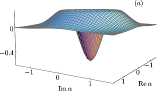
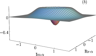
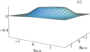
Figure 1: Wigner function of the quantum state of the pulse that leaves the cavity, the mode of which is (initially) prepared in a single-photon state. (a) $\eta(t)$ $\!=$ $\!0.99$; (b) $\eta(t)$ $\!=$ $\!0.71$; (c) $\eta(t)$ $\!=$ $\!0.5$.

Setting in Eq. (54) $s$ $\!=$ $\!s_{0}$ $\!=$ $\!0$, we see that the Wigner function of the relevant output mode is the following convolution of the Wigner function of the cavity mode with a Gaussian:

$$W_{\mathrm{out}}(\alpha,t)=\frac{2}{\pi}\frac{1}{1-\eta(t)}$$ (62)

$$\;\times\,\int\mbox{\rm d}^{2}\beta\,W_{\mathrm{cav}}(\beta)\,\exp\!\left[-\frac{2|\sqrt{\eta(t)}\beta-\alpha|^{2}}{1-\eta(t)}\right]\!.\quad$$

This equation reveals that for perfectly extracting a quantum state from a high-$Q$ cavity, the condition

$$\frac{\eta(t)}{1-\eta(t)}\gg 1$$ (63)

should be satisfied, i.e., the value of the extraction efficiency $\eta(t)$ must be sufficiently close to unity. How close to unity – it really depends on the characteristic quantum features of the state to be extracted. On the other hand, from Eq. (61) it follows that

$$\eta(t)\leq\frac{\gamma_{\mathrm{rad}}}{\gamma_{\mathrm{rad}}+\gamma_{\mathrm{abs}}}\,.$$ (64)

Note that $\eta(t)$ $\!\simeq$ $\!\gamma_{\mathrm{rad}}/(\gamma_{\mathrm{rad}}$ $\!+$ $\!\gamma_{\mathrm{abs}})$ for sufficiently long times $t$ $\!-$ $\!t_{0}$ $\!\gtrapprox$ $\!(\gamma_{\mathrm{rad}}$ $\!+$ $\!\gamma_{\mathrm{abs}})^{-1}$.

IV Examples

The really required efficiency for nearly perfect quantum state extraction sensitively depends on the quantum state that is desired to be extracted. To illustrate this, let us consider two examples of highly nonclassical states, namely Fock states and Schrödinger catlike states.

IV.1 Fock states

A typical nonclassical state is an $n$-photon Fock state, whose Wigner function reads

$$W_{\mathrm{cav}}^{(n)}(\alpha)=\frac{2}{\pi}(-1)^{n}e^{-2|\alpha|^{2}}\mathrm{L}_{n}\!\left(4|\alpha|^{2}\right),$$ (65)

where $\mathrm{L}_{n}(x)$ is the Laguerre polynomial of order $n$. Substituting Eq. (65) into Eq. (62) and employing the integral representation of the Laguerre polynomials Arfken ,

$$\mathrm{L}_{n}\!\left(x\right)=\frac{1}{2\pi i}\oint_{\gamma}\mbox{\rm d}z\,\frac{e^{-xz/(1-z)}}{z^{n+1}(1-z)}\,,$$ (66)

where the contour $\gamma$ encloses the origin but not the point $z=1$, after straightforward calculations we obtain the Wigner function of the output pulse as

$$W_{\mathrm{out}}^{(n)}(\alpha,t)=\frac{2}{\pi}(-1)^{n}\,e^{-2|\alpha|^{2}}\left[2\eta(t)-1\right]^{n}$$ (67)

$$\hskip 43.05542pt\times\,\mathrm{L}_{n}\!\left[\frac{4\eta(t)}{2\eta(t)-1}|\alpha|^{2}\right].$$

From Eq. (67) it is not difficult to see that the condition

$$\eta(t)>1-\frac{1}{2n}$$ (68)

must be satisfied to guarantee that the $n$-photon Fock state prevails in the mixed output quantum state. In the simplest case of a one-photon Fock state, $n$ $\!=$ $\!1$, the condition reduces to $\eta(t)$ $\!>$ $\!0.5$. That is to say, the weight of the one-photon Fock state exceeds the weight of the vacuum state in the mixed state of the outgoing field,

$$W_{\mathrm{out}}^{(1)}(\alpha,t)=[1-\eta(t)]W^{(0)}(\alpha)+\eta(t)W^{(1)}(\alpha),$$ (69)

only if the extraction efficiency exceeds $50\%$. The condition (68) clearly shows that with increasing value of $n$ the required extraction efficiency rapidly approaches $100\%$.

The dependence on the extraction efficiency of the quantum state of the outgoing field is illustrated in Fig. 1 for the case in which a single-photon Fock state is desired to be extracted. Figure 1(a) reveals that nearly perfect extraction requires an extraction efficiency that should be not smaller than $\eta(t)$ $\!=$ $\!0.99$, which for $t$ $\!\to$ $\!\infty$ corresponds to the requirement that $\gamma_{\mathrm{abs}}/\gamma_{\mathrm{rad}}$ $\!\lesssim$ $\!0.01$. As long as $\eta(t)$ $\!>$ $\!0.5$, the single-photon Fock state is the dominant state in the mixed output state, as can be seen from Fig. 1(b) [$\eta(t)$ $\!=$ $\!0.71$, i.e., $\gamma_{\mathrm{abs}}/\gamma_{\mathrm{rad}}$ $\!=$ $\!0.429$ ($t$ $\!\to$ $\!\infty$)]. For $\eta(t)$ $\!\leq$ $\!0.5$, i.e., $\gamma_{\mathrm{abs}}/\gamma_{\mathrm{rad}}$ $\!\geq$ $\!1$ ($t$ $\!\to$ $\!\infty$)], the features typical of a single-photon Fock state are lost, Fig. 1(c).

IV.2 Schrödinger catlike states

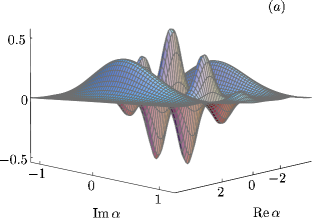
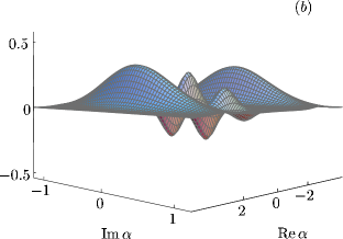
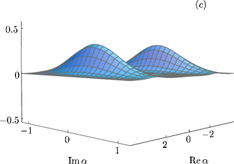
Figure 2: Wigner function of the quantum state of the pulse that leaves the cavity, the mode of which is (initially) prepared in a Schrödinger catlike state given by Eq. (70) with $\alpha_{0}$ $\!=$ $\!3$. (a) $\eta(t)$ $\!=$ $\!0.998$; (b) $\eta(t)$ $\!=$ $\!0.952$; (c) $\eta(t)$ $\!=$ $\!0.84$.

Another example of typically nonclassical states are Schrödinger catlike states, e.g.,

$$\left|\psi\right\rangle_{\mathrm{cav}}=\mathcal{N}\left(\left|\alpha_{0}\right\rangle+\left|-\alpha_{0}\right\rangle\right),$$ (70)

with $\alpha_{0}$ real, and

$$\mathcal{N}=\left[2\left(1+\,e^{-4\alpha_{0}^{2}}\right)\right]^{-1/2}\,.$$ (71)

The Wigner function of such a state is given by

$$W_{\mathrm{cav}}(\alpha)=\frac{2\mathcal{N}^{2}}{\pi}\left[e^{-2|\alpha-\alpha_{0}|^{2}}\right.$$ (72)

$$\left.+\,e^{-2|\alpha+\alpha_{0}|^{2}}+2\,e^{-2|\alpha|^{2}}\cos\!\left(4\alpha_{0}\mathrm{Im}\,\alpha\right)\right].$$

Substitution of Eq. (72) into Eq. (62) yields the following expression for the Wigner function of the output fields:

$$W_{\mathrm{out}}(\alpha,t)=\frac{2\mathcal{N}^{2}}{\pi}$$ (73)

$$\times\,\left\{e^{-2|\alpha-\sqrt{\eta(t)}\alpha_{0}|^{2}}+e^{-2|\alpha+\sqrt{\eta(t)}\alpha_{0}|^{2}}\right.$$

$$\left.+\,2e^{-2|\alpha|^{2}}\cos\left[4\sqrt{\eta(t)}\alpha_{0}\mathrm{Im}\,\alpha\right]e^{-2\alpha_{0}^{2}[1-\eta(t)]}\right\}.\quad$$

From Eq. (73) it follows that nearly perfect extraction of the state requires the condition

$$1-\eta(t)\ll\frac{1}{2|\alpha_{0}|^{2}}$$ (74)

to be satisfied.

Figure 2 illustrates the dependence on the extraction efficiency of the quantum state of the outgoing field for a Schrödinger catlike cavity state with $\alpha_{0}$ $\!=$ $\!3$. Comparing Fig. 2 with Fig. 1, we see that, as expected, the efficiency for extracting such a Schrödinger catlike state is required to be substantially higher than that for extracting a single-photon Fock state. For a nearly perfect extraction of the chosen Schrödinger catlike state, the efficiency should be not smaller than $\eta(t)$ $\!=$ $\!0.998$, i.e., $\gamma_{\mathrm{abs}}/\gamma_{\mathrm{rad}}$ $\!\lesssim$ $\!0.002$ for $t$ $\!\to$ $\!\infty$ [Fig 2(a)]. The nonclassical interference fringes typical of a Schrödinger catlike state can be observed, at least rudimentarily, as long as $\eta(t)$ $\!>$ $\!0.84$, i.e., $\gamma_{\mathrm{abs}}/\gamma_{\mathrm{rad}}$ $\!<$ $\!0.19$ ($t$ $\!\to$ $\!\infty$) [Fig 2(b); $\eta(t)$ $\!=$ $\!0.952$, i.e.,$\gamma_{\mathrm{abs}}/\gamma_{\mathrm{rad}}$ $\!=$ $\!0.05$ ($t$ $\!\to$ $\!\infty$)]. For smaller values of the extraction efficiency, the quantum interferences are effectively destroyed [Fig. 2(c)].

V Summary and Conclusions

We have derived an input-output relation that relates the quantum state of the pulse leaving a high-$Q$ cavity to the quantum state in which an excited cavity mode was prepared at some initial time. Performing the calculations in the phase space, we have represented the respective quantum states in terms of $s$-parametrized phase-space functions and derived a formula that relates the phase-space functions of the outgoing field and the cavity mode to each other. Taking into account unwanted losses of the cavity mode, we have studied the conditions under which a nearly perfect extraction of non-classical quantum states from high-$Q$ cavities should be possible.

To calculate the quantum state of the outgoing field, we started from its time-dependent continuous multimode characteristic functional. By appropriate diagonalization, it can be rewritten in terms of non-monochromatic modes, one of which is related to the cavity mode, while all other modes remain unaffected by the cavity mode. In this way, the $s$-parametrized phase-space functions of the quantum state of the relevant non-monochromatic output mode can be expressed in terms of $s$-parametrized phase-space functions of the quantum state in which the cavity mode was prepared. In particular, the output Wigner function can be given as a convolution of the cavity Wigner function with a Gaussian reflecting the unwanted losses.

The crucial parameter for nearly perfect extraction of a quantum state from a high-$Q$ cavity is the extraction efficiency, which in the long-time limit is determined by the ratio between the cavity-mode decay rate due to unwanted losses and the cavity-mode decay rate due to wanted (i.e., transmission) losses. This ratio must be sufficiently small in order to realize a nearly $100\%$ extraction efficiency, where the really required smallness sensitively depends on the quantum state to be exctracted. In particular, extracting highly nonclassical states can require extremely small values of this ratio.

It should be pointed out that even for the best optical high-$Q$ microcavities available the required efficiencies for nearly perfect extraction of nonclassical quantum states have not been reached, because the unwanted losses are of the same order of magnitude as the transmission losses Rempe92 ; Hood01 ; Pelton02 . So, in the simplest case of extracting from a cavity a one-photon Fock state, the weight of the one-photon Fock state exceeds the weight of the vacuum state in the mixed output quantum state only if the extraction efficiency is bigger than $50\%$. However, the biggest value that has been realized so far in the production of triggered single photons by coupling a single semiconductor quantum dot to an optical mode in a micropost microcavity is about $38\%$ Pelton02 . On the contrary, in case of high-$Q$ microwave cavities the absorption losses may be small compared with the transmission losses Walther03 .

We have concentrated on the calculation of the quantum state of the field that leaves a single cavity that is initially excited in some single-mode quantum state. The theory can also be extended to multimode excitation in a single cavity as well as multi-cavity systems. We have further assumed that the input field is in the vacuum quantum state. Clearly, the underlying formalism can also be applied to the case, in which the input field is prepared in another than the vacuum state. Needless to say that when the input field is in a thermal state, then additional noise is fed into the cavity, and the quantum state of the output field also carries additional noise. As can be seen from Eq. (16), the operator input-output relation used in this paper does not take into account that the input field could be absorbed in the entrance port of the cavity, which would also give rise to additional noise. To include this effect in the theory, the input-output relation (16) should be generalized, e.g., by following the line in Ref. Khanbekyan03 .

Finally, we have assumed that the process of preparation of the quantum state of the cavity mode is sufficiently short compared with the decay time of the cavity mode, so that the time scales of quantum state preparation and extraction are well separated from each other and the preparation process can be ignored in the calculations. At this point it should be mentioned that one possible way to reduce the effect of unwanted losses may be the use of cavities of deliberately enlarged transmission, so that the unwanted losses become small compared with transmission losses. When, for example, the radius of a microsphere cavity is diminished, then the transmission losses increase, thereby the absorption losses remaining nearly constant Ho01 ; Buck03 . Since, on the other hand, the quality factor is reduced, the preparation time may be comparable with the cavity decay time, which is now determined by the transmission time. So, in the single-photon emitter experiments in Ref. Kuhn02 , in which a cavity of a $Q$ value of $6\!\times\!10^{4}$ is used, the measured transmission time of several microseconds is of the same order of magnitude as the cavity decay time. In order to answer the question of which quantum state is really obtained outside the cavity in such a case, the preparation process must necessarily be included in the calculations.

- (1) J. M. Raimond, M. Brune, and S. Haroche, Rev. Mod. Phys. 73, 565 (2001).
- (2) P. W. H. Pinkse, T. Fischer, P. Maunz, and G. Rempe, Nature 404, 365 (2000).
- (3) C. J. Hood, T. W. Lynn, A. C. Doherty, A. S. Parkins, and H. J. Kimble, Science 287, 1447 (2000).
- (4) A. C. Doherty, T. W. Lynn, C. J. Hood, and H. J. Kimble, Phys. Rev. A 63, 013401 (2000).
- (5) E. Knill, R. Laflamme, and G. J. Milburn, Nature 409, 46 (2001).
- (6) S. J. Enk, J. I. Cirac, and P. Zoller, Science 279, 205 (1998).
- (7) B. Tregenna, A. Beige, and P. L. Knight, Phys. Rev. A 65, 032305 (2002).
- (8) J.-W. Pan, S. Gasparoni, R. Ursin, G. Weihs, and A. Zeilinger, Nature 423, 417 (2003).
- (9) C. H. Bennett and D. P. DiVincenzo, Nature 404, 247 (2000).
- (10) F. De Martini, G. Di Giuseppe, and M. Marrocco, Phys. Rev. Lett. 76, 900 (1996).
- (11) A. Rauschenbeutel, P. Bertet, S. Osnaghi, G. Nogues, M. Brune, J. M. Raimond, and S. Haroche, Phys. Rev. A 64, 050301(R) (2001).
- (12) D. E. Browne and M. B. Plenio, Phys. Rev. A 67, 012325 (2003).
- (13) P. Domokos, M. Brune, J. M. Raimond, and S. Haroche, Eur. Phys. J. D 1, 1 (1998).
- (14) S. Brattke, B. T. H. Varcoe, and H. Walther, Phys. Rev. Lett. 86, 3534 (2001).
- (15) E. Solano, G. S. Agarwal, and H. Walther, Phys. Rev. Lett. 90, 027903 (2003).
- (16) A. S. Parkins, P. Marte, P. Zoller, O. Carnal, and H. J. Kimble, Phys. Rev. A 51, 1578 (1995).
- (17) M. Hennrich, T. Legero, A. Kuhn, and G. Rempe Phys. Rev. Lett. 85, 4872 (2000).
- (18) W. Lange and H. J. Kimble, Phys. Rev. A 61, 063817 (2000).
- (19) L.-M. Duan, A. Kuzmich, and H. J. Kimble, Phys. Rev. A 67, 032305 (2003).
- (20) J. I. Cirac, P. Zoller, H. J. Kimble, and H. Mabuchi, Phys. Rev. Lett. 78, 3221 (1997).
- (21) S. Zippilli, D. Vitali, P. Tombesi, and J.-M. Raimond, Phys. Rev. A 67, 052101 (2003).
- (22) A. Kuhn, M. Hennrich, and G. Rempe, Phys. Rev. Lett. 89, 067901 (2002).
- (23) G. Rempe, R. J. Thompson, and H. Kimble, Opt. Lett. 17, 363 (1992); G. Rempe, private communication (2003).
- (24) C. J. Hood, H. J. Kimble, and Jun Ye, Phys. Rev. A 64, 033804 (2001).
- (25) M. Pelton, C. Santori, J. Vučković, B. Zhang, G. S. Solomon, J. Plant, and Yoshihisa Yamamoto, Phys. Rev. Lett. 89, 233602 (2002).
- (26) C. Saavedra, K. M. Gheri, P. Törmä, J. I. Cirac, and P. Zoller, Phys. Rev. A 61, 062311 (2000).
- (27) S. Scheel and D.-G. Welsch, Phys. Rev. A 64, 063811 (2001).
- (28) M. França Santos, L. G. Lutterbach, S. M. Dutra, N. Zagury, and L. Davidovich, Phys. Rev. A 63, 033813 (2001).
- (29) C. W. Gardiner and M. J. Collett, Phys. Rev. A 31, 3761 (1985).
- (30) L. Knöll, W. Vogel, and D.-G. Welsch, Phys. Rev. A 43, 543 (1991).
- (31) W. Vogel and D.-G. Welsch, Lectures on Quantum Optics, Akademie Verlag GmbH, Berlin / VCH Publishers, Inc., New York, (1994).
- (32) H. Walther, private communication (2003).
- (33) M. Khanbekyan, L. Knöll, and D.-G. Welsch, Phys. Rev. A 67, 063812 (2003).
- (34) G. Arfken, Mathematical Methods for Physicists, Academic Press, Orlando, (1985).
- (35) Ho Trung Dung, L. Knöll, and D.-G. Welsch, Phys. Rev. A 64, 013804 (2001).
- (36) J. R. Buck and H. J. Kimble, Phys. Rev. A 67, 033806 (2003).