Quantum dot single photon sources: Prospects for applications in linear optics quantum information processing

Abstract

An optical source that produces single photon pulses on demand has potential applications in linear optics quantum computation, provided that stringent requirements on indistinguishability and collection efficiency of the generated photons are met. We show that these are conflicting requirements for anharmonic emitters that are incoherently pumped via reservoirs. As a model for a coherently pumped single photon source, we consider cavity-assisted spin-flip Raman transitions in a single charged quantum dot embedded in a microcavity. We demonstrate that using such a source, arbitrarily high collection efficiency and indistinguishability of the generated photons can be obtained simultaneously with increased cavity coupling. We analyze the role of errors that arise from distinguishability of the single photon pulses in linear optics quantum gates by relating the gate fidelity to the strength of the two-photon interference dip in photon cross-correlation measurements. We find that performing controlled phase operations with error $<1\%$ requires nano-cavities with Purcell factors $F_{P}\geq 40$ in the absence of dephasing, without necessitating the strong coupling limit.

I Introduction

A significant fraction of key experiments in the emerging field of quantum information science Nielsen and Chuang (2000), such as Bell’s inequality violations Aspect (1999), quantum key distribution Bennett et al. (1992); Ekert et al. (1992) and quantum teleportation Bouwmeester et al. (1997) have been carried out using single photon pulses and linear optical elements such as polarizers and beam splitters. However, it was generally assumed that in the absence of photon-photon interactions, the role of optics could not be extended beyond these rather limited applications. Recently, Knill, Laflamme, and Milburn have shown theoretically that efficient linear optics quantum computation (LOQC) can be implemented using on-demand indistinguishable single-photon pulses and high-efficiency photon-counters Knill et al. (2001). This unexpected result has initiated a number of experimental efforts aimed at realizing suitable single-photon sources. Impressive results demonstrating a relatively high degree of indistinguishability and collection efficiency have been obtained using a single quantum dot embedded in a microcavity Santori et al. (2002). Two-photon interference has also been observed using a single cold atom trapped in a high-Q Fabry-Perot cavity Rempe (2003). A necessary but not sufficient condition for obtaining indistinguishable single photons on demand is that the cavity-emitter coherent coupling strength ($g$) exceeds the square root of the product of the cavity ($\kappa_{cav}$) and emitter ($\gamma$) coherence decay rates. When the emitter is spontaneous emission broadened and the cavity decay dominates over other rates, this requirement corresponds to the Purcell regime ($g^{2}/\kappa_{cav}\gamma>1$).

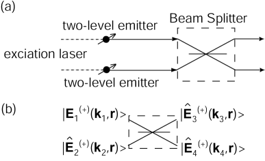
Figure 1: (a) Configuration assumed in the analysis of two-photon interference: Two independent identical single photon sources excited by the same laser field. (b) Input and output fields of the beam splitter.

In this paper, we identify the necessary and sufficient conditions for generation of single photon pulses with an arbitrarily high collection efficiency and indistinguishability. While our results apply to all single-photon sources based on two-level emitters, our focus will be on quantum dot based devices. First, we show that single photon sources that rely on incoherent excitation of a single quantum dot (through a reservoir) cannot provide high collection efficiency and indistinguishability, simultaneously. To achieve this goal, the only reservoir that the emitter couples to has to be the radiation field reservoir that induces the cavity decay. We show that a source based on cavity-assisted spin-flip Raman transition satisfies this requirement and can be used to generate the requisite single-photon pulses in the Purcell regime. This analysis is done in section II where we calculate the degree of interference (indistinguishability) of two photons and the theoretical maximum collection efficiency, as a function of the cavity coupling strength, laser pulsewidth, and emitter dephasing rate for different single photon sources.

Interference of two single-photon pulses on a beam-splitter plays a central role in all protocols for implementing indeterministic two-qubit gates, which are in turn key elements of linear optics quantum computation schemes Knill et al. (2001). Observability of two-photon interference effects naturally requires that the two single-photons arriving at the two input ports of the beam-splitter be indistinguishable in terms of their pulsewidth, bandwidth, polarization, carrier frequency, and arrival time at the beam-splitter. The first two conditions are met for an ensemble of single-photon pulses that are Fourier-transform limited: this is the case if the source (single atom or quantum dot) transition is broadened solely by spontaneous emission process that generates the photons. While the radiative lifetime (i.e. the single-photon pulsewidth) of the emitter does not affect the observability of interference, any other mechanism that allows one to distinguish the two photons will. A simple example that is relevant for quantum dot single photon sources is the uncertainty in photon arrival (i.e. emission) time arising from the random excitation of the excited state of the emitter transition: if for example this excited state is populated by spontaneous phonon emission occuring with a waiting time of $\tau_{relax}$, then the starting time of the photon generation process will have a corresponding time uncertainty of $\sim\tau_{relax}$. We refer to this uncertainty as time-jitter. Since the information about the photon arrival time is now carried by the phonon reservoir, the interference will be degraded.

Even though the role of single-photon loss on linear optics quantum computation has been analyzed Knill et al. (2001), there has been to date no analysis of gate errors arising from distinguishability of single photons. To this end, we first note that while various sources of distinguishability can be eliminated, the inherent jitter in photon emission time remains as an unavoidable source of distinguishability. Hence, in section III, we analyze the performance of a linear-optics-controlled phase gate in the presence of time-jitter and relate the gate fidelity to the degree of indistinguishability of the generated photons, as measured by a Hong-Ou-Mandel Hong et al. (1987) type two-photon interference experiment.

II Maximum collection efficiency and indistinguishability of photons generated by single photon sources

In this section we first develop the general formalism for calculating a normalized measure of two-photon interference based on the projection operators of a two-level emitter. We then compare and contrast the case where the emitter is pumped via spontaneous emission of a photon or a phonon from an excited state, i.e. an incoherently pumped single photon source, to the case where single photon pulses are generated by cavity-assisted spin-flip Raman scattering, i.e. coherently pumped single photon source.

Previous analysis of two-photon interference among photons emitted from single emitters were carried out for two-level systems driven by a cw laser field Fearn and Loudon (1989); Bylander et al. (2003). In contrast, we treat the pulsed excitation, and analyze currently available single photon sources based on two and three-level emitters. We note that extensive analysis of two-photon interference phenomenon was carried out for twin photons generated by parametric down conversion Ghosh et al. (1986); Hong et al. (1987); Shih and Alley (1988); Steinberg et al. (1992), and single photon wave-packets Legero et al. (2003), without considering the microscopic properties of the emitter.

II.1 Calculation of the degree of two-photon interference

We consider the experimental configuration depicted in Figure 1(a). Two general independent identical two-level emitters are assumed to be excited by the same laser. We assert no further assumptions on two-level emitters; they are considered to be light sources that exhibit perfect photon antibunching. Single photons emitted from the two-level emitters are coupled to different inputs of a beam splitter which is equidistant from both sources. In the ideal scenario where the input channels are mode-matched and the incoming photons have identical spectral and spatial distributions, two-photon interference reveals itself in lack of coincidence counts among the two output channels. This bunching behavior is a signature of the bosonic nature of photons.

Recent demonstration of two-photon interference using a single quantum dot single photon source relied on a similar scheme based on a Michelson interferometer Santori et al. (2002). In this experiment, the interferometer had a large path length difference between its two branches. Such a difference, in excess of single photon coherence length, provided the interference among photons subsequently emitted from the same source. Two-photon interference in this experiment is quantitatively similar to interference obtained among photons emitted by two different identical sources.

Input-output relationships for single mode photon annihilation operators in the beam splitter (Fig. 1(b)) are defined by the unitary operation

$$\left[\begin{array}[]{c}\hat{a}_{3}(\omega)\\ \hat{a}_{4}(\omega)\end{array}\right]=\left[\begin{array}[]{cc}\cos\xi&-e^{-i\phi}\sin\xi\\ e^{i\phi}\sin\xi&\cos\xi\end{array}\right]\left[\begin{array}[]{c}\hat{a}_{1}(\omega)\\ \hat{a}_{2}(\omega)\end{array}\right]\,.$$ (7)

$\hat{a}_{1}(\omega)$, $\hat{a}_{2}(\omega)$, $\hat{a}_{3}(\omega)$, and $\hat{a}_{4}(\omega)$ represent single mode photon annihilation operators in channels $\mathbf{k_{1}}$, $\mathbf{k_{2}}$, $\mathbf{k_{3}}$, and $\mathbf{k_{4}}$ respectively. $\mathbf{k_{1}}$, $\mathbf{k_{2}}$, $\mathbf{k_{3}}$, and $\mathbf{k_{4}}$ have identical amplitudes and polarizations while satisfying the momentum conservation. We will abbreviate the unitary operation in the beam splitter as $u(\textbf{B}_{\xi,\phi})$.

Assuming that $u(\textbf{B}_{\xi,\phi})$ is constant over the frequency range of consideration, Eq. (7) can be Fourier transformed to reveal

$$\left[\begin{array}[]{c}\hat{a}_{3}(t)\\ \hat{a}_{4}(t)\end{array}\right]=u(\textbf{B}_{\xi,\phi})\left[\begin{array}[]{c}\hat{a}_{1}(t)\\ \hat{a}_{2}(t)\end{array}\right]\,.$$ (12)

$\hat{a}_{1}(t)$, $\hat{a}_{2}(t)$, $\hat{a}_{3}(t)$, and $\hat{a}_{4}(t)$ now represent time dependent photon annihilation operators.

Coincidence events at the output of the beam splitter are quantified by the cross-correlation function between channels 3 and 4 which is given by

$$G^{(2)}_{34}(t,\tau) = \langle\hat{a}_{3}^{\dagger}(t)\hat{a}_{4}^{\dagger}(t+\tau)\hat{a}_{4}(t+\tau)\hat{a}_{3}(t)\rangle\,,$$ (13)

$$g^{(2)}_{34}(t,\tau) = \frac{G^{(2)}_{34}(t,\tau)}{\langle\hat{a}_{3}^{\dagger}(t)\hat{a}_{3}(t)\rangle\langle\hat{a}_{4}^{\dagger}(t+\tau)\hat{a}_{4}(t+\tau)\rangle}\,,$$ (14)

in its unnormalized ($G^{(2)}_{34}(t,\tau)$) and normalized ($g^{(2)}_{34}(t,\tau)$) form. By substitution of Eq. (12) in (13), $G^{(2)}_{34}(t,\tau)$ is expressed as

$$G^{(2)}_{34}(t,\tau) = \sin^{4}\xi\langle\hat{a}_{2}^{\dagger}(t)\hat{a}_{1}^{\dagger}(t+\tau)\hat{a}_{1}(t+\tau)\hat{a}_{2}(t)\rangle$$ (15)

$$+ \cos^{4}\xi\langle\hat{a}_{1}^{\dagger}(t)\hat{a}_{2}^{\dagger}(t+\tau)\hat{a}_{2}(t+\tau)\hat{a}_{1}(t)\rangle$$

$$- \cos^{2}\xi\sin^{2}\xi\left(\langle\hat{a}_{1}^{\dagger}(t)\hat{a}_{2}^{\dagger}(t+\tau)\hat{a}_{1}(t+\tau)\hat{a}_{2}(t)\rangle\right.$$

$$+ \left.\langle\hat{a}_{2}^{\dagger}(t)\hat{a}_{1}^{\dagger}(t+\tau)\hat{a}_{2}(t+\tau)\hat{a}_{1}(t)\rangle\right)\,.$$

In what follows we assume ideal mode-matched beams in inputs 1 and 2. Hence the bracket notation corresponds to time expectations only.

In Eq. (15), photon annihilation operators of channels 1 and 2 are due to the radiation field of a general single two-level emitter. In the far field, this field annihilation operator is given by the source-field relationship as

$$\hat{a}(t)=A(\mathbf{r})\hat{\sigma}_{ge}\left(t-\frac{\left|\mathbf{r}\right|}{c}\right)\,,$$ (16)

where $A(\mathbf{r})$ is a time-independent proportionality factor Loudon (1983). This linear relationship allows for substitution of photon annihilation and creation operators by dipole projection operators $\hat{\sigma}_{ge}$ and $\hat{\sigma}_{eg}$ respectively in Eq. (15). Using the assumption that both of the emitters are independent and have identical expectation values and coherence functions, we arrive at

$$G^{(2)}_{34}(t,\tau) = \left[\left(\cos^{4}\xi+\sin^{4}\xi\right)\langle\hat{\sigma}_{ee}(t)\rangle\langle\hat{\sigma}_{ee}(t+\tau)\rangle\right.$$ (17)

$$-2\cos^{2}\xi\sin^{2}\xi|\widetilde{G}^{(1)}(t,\tau)|^{2}]\,\left|A(\mathbf{r})\right|^{4}\,.$$

In this equation $\widetilde{G}^{(1)}(t,\tau)$ represents the unnormalized first-order coherence function

$$\widetilde{G}^{(1)}(t,\tau)=\langle\hat{\sigma}_{eg}(t+\tau)\hat{\sigma}_{ge}(t)\rangle\,.$$ (18)

For a balanced beam-splitter, $\theta=\pi/4$, Eq. (17) simplifies to

$$\widetilde{G}^{(2)}_{34}(t,\tau) \equiv \frac{G^{(2)}_{34}(t,\tau)}{|A(\mathbf{r})|^{4}}$$ (19)

$$= \frac{1}{2}\left(\langle\hat{\sigma}_{ee}(t)\rangle\langle\hat{\sigma}_{ee}(t+\tau)\rangle-|\widetilde{G}^{(1)}(t,\tau)|^{2}\right)\,.$$

This is the expression of the unnormalized second order coherence function in terms of the dipole projection operators that we will use in the remaining of this section.

Under pulsed excitation further considerations need to be taken into account to normalize this equation. Before this discussion however, we note that under continuous wave excitation, Eq. (14) reveals the normalized second order coherence function

$$g^{(2)}_{34}(t,\tau) = \frac{1}{2}\left(1-\frac{\left|\widetilde{G}^{(1)}(t,\tau)\right|^{2}}{\langle\hat{\sigma}_{ee}(t)\rangle_{ss}^{2}}\right)$$ (20)

$$= \frac{1}{2}\left(1-\left|g^{(1)}(\tau)\right|^{2}\right)\,,$$

where $\langle\hat{\sigma}_{ee}(t)\rangle_{ss}$ represents the steady state population density of the excited state.

Figure 2: Unnormalized coincidence detection rate, $\widetilde{G}^{(2)}_{34\_exp}$, of an incoherently pumped quantum dot. Parameter values are: $\Gamma_{relax}=100\Gamma_{spon}$, $\gamma_{deph}=\Gamma_{spon}$, each laser pulse is a Gaussian with pulsewidth $0.05/\Gamma_{spon}$ and peak Rabi frequency $35\Gamma_{spon}$.

Experimental determination of the cross-correlation function relies on ensemble averaging coincidence detection events. Hanbury Brown and Twiss setup is frequently used in these experiments where the experimentally relevant cross-correlation function

$$\widetilde{G}^{(2)}_{34\_exp}(\tau)=\lim_{T\rightarrow\infty}\int_{0}^{T}{\widetilde{G}^{(2)}_{34}(t,\tau)\,dt}\,,$$ (21)

is measured. The total detection time $T$ is long compared to the single photon pulsewidth ($T\rightarrow\infty$) in these experiments.

In Fig. 2 we plot an exemplary calculation of $\widetilde{G}^{(2)}_{34\_exp}(\tau)$ for an incoherently pumped, dephased quantum dot considering a series of 6 pulses. This calculation is done by the integration of $\widetilde{G}^{(2)}_{34}(t,\tau)$ (Eq. (21)), while $\widetilde{G}^{(2)}_{34}(t,\tau)$ is calculated using the optical Bloch equations and the quantum regression theorem. We will detail these calculations in the following subsections. In such calculations, the area of the peak around $\tau\sim 0$ ($0^{th}$ peak) gives the unnormalized coincidence detection probability when two photons are incident in different inputs of the beam splitter. This area should be normalized by the area of the other peaks: Absence of two-photon interference implies $0^{th}$ peak and other peaks to be identical, whereas in total two-photon interference, $0^{th}$ peak has vanishing area. This normalized measure of two-photon interference is

$$p_{34} = \frac{\int_{t=0}^{\infty}\int_{\tau,0}{\widetilde{G}^{(2)}_{34}(t,\tau)\,dt\,d\tau}}{\int_{t=0}^{\infty}\int_{\tau,n}\widetilde{G}^{(2)}_{34}(t,\tau)\,dt\,d\tau}\,.$$ (22)

In the numerator, integral in $\tau$ is taken over the $0^{th}$ peak, whereas in the denominator this integral is taken over the $n^{th}$ peak where $n=\pm 1,\pm 2,...$.

We now simplify Eq. (22) further using the periodicity with respect to $\tau$ and $t$. First simplification is due to periodicity in $\tau$ which is apparent in the periodicity of the peaks other than $0^{th}$ peak in Fig. 2. The area of these peaks is given by

$$\int_{0}^{\infty}{\langle\hat{\sigma}_{ee}(t)\rangle\langle\hat{\sigma}_{ee}(t+\tau-nT_{pulse})\rangle\,dt}\,,$$ (23)

for $n=\pm 1,\pm 2,...$ This is due to the vanishing $\widetilde{G}^{(1)}(t,\tau)$ for absolute delay times larger than single photon coherence time. Hence the normalized coincidence probability can also be represented as

$$p_{34} = \frac{\int_{t=0}^{\infty}\int_{\tau,0}{\widetilde{G}^{(2)}_{34}(t,\tau)\,dt\,d\tau}}{\int_{t=0}^{\infty}\int_{\tau,0}\langle\hat{\sigma}_{ee}(t)\rangle\langle\hat{\sigma}_{ee}(t+\tau)\rangle\,dt\,d\tau}\,.$$ (24)

Periodicity of $\widetilde{G}^{(2)}_{34}(t,\tau)$ and $\langle\hat{\sigma}_{ee}(t)\rangle\langle\hat{\sigma}_{ee}(t+\tau)\rangle$ in $t$ further simplifies Eq. (24) to

$$p_{34} = \frac{N\int_{t=0}^{T_{pulse}}\int_{\tau,0}{\widetilde{G}^{(2)}_{34}(t,\tau)\,dt\,d\tau}}{N\int_{t=0}^{T_{pulse}}\int_{\tau,0}\langle\hat{\sigma}_{ee}(t)\rangle\langle\hat{\sigma}_{ee}(t+\tau)\rangle\,dt\,d\tau}$$ (25)

$$= \frac{\int_{t=0}^{T_{pulse}}\int_{\tau,0}{\widetilde{G}^{(2)}_{34}(t,\tau)\,dt\,d\tau}}{\int_{t=0}^{T_{pulse}}\int_{\tau,0}\langle\hat{\sigma}_{ee}(t)\rangle\langle\hat{\sigma}_{ee}(t+\tau)\rangle\,dt\,d\tau}\,,$$

where N represents the number of pulses considered in the calculation.

Eq. (25) is the final result of the simplifications and is used in the rest of this section. It is important to note that this equation enables us to obtain the normalized coincidence probability, $p_{34}$, by considering only a single laser pulse. This greatly improves the efficiency of the simulations.

There are two limitations of our method of calculation. Firstly, the optical Bloch equation description does not take into account laser broadening induced by amplitude or phase fluctuations. Secondly, in the case of a quantum dot, an upper limit to laser broadening may arise due to the biexciton splitting ($\sim 3.5~{}meV$ at cryogenic temperatures) and Zeeman splitting ($\sim 1~{}meV$ for an applied field of 10 Tesla). Overall, these restrictions should put a lower limit of $\sim 1\times 10^{-12}$ s to the laser pulsewidth. This lower limit is always exceeded in our calculations.

II.2 Single photon source based on an incoherently pumped quantum dot

Various demonstrations of single photon sources based on solid-state emitters have been reported in recent years. Single quantum dots Michler et al. (2000); Santori et al. (2001); Zwiller et al. (2001); Moreau et al. (2001); Yuan et al. (2002), single molecules Martini et al. (1996); Brunel et al. (1999); Lounis and Moerner (2000), and single N vacancies Kurtsiefer et al. (2000); Beveratos et al. (2001) were used in these demonstrations where pulsed excitation of a high energy state followed by a fast relaxation and excited state recombination proved to be a very convenient method to generate triggered single photons. This method of incoherent pumping ensured the detection of at most one photon per pulse, provided that the laser had sufficiently short pulses, and large pulse separations.

In the following, we extensively consider the case of quantum dots and analyze two-photon interference among photons emitted from an incoherently pumped quantum dot. In such a three-level scheme (Fig. 3), time-jitter induced by the fast relaxation ($\Gamma_{relax}$) and dephasing in $|e\rangle$-$|g\rangle$ transition are the sources of non-ideal two-photon interference. We investigate these effects first under continuous wave, then under pulsed excitation.

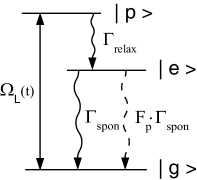
Figure 3: Model of an incoherently pumped single quantum dot. Dashed line demonstrates the generated single photons via cavity leakage.

II.2.1 Continuous wave excitation

Under continuous wave excitation, $\widetilde{G}^{(1)}(t,\tau)$ is calculated by applying quantum regression theorem Loudon (1983) to the optical Bloch equation for $\langle\hat{\sigma}_{eg}(t)\rangle$, revealing

$$\frac{d\widetilde{G}^{(1)}(t,\tau)}{d\tau}=-\gamma\widetilde{G}^{(1)}(t,\tau)\,,$$ (26)

where $\gamma=\frac{\Gamma_{spon}}{2}+\gamma_{deph}$ is the total coherence decay rate of $|e\rangle$-$|g\rangle$ transition. Here $\gamma_{deph}$ denotes dephasing caused by all reservoirs other than that of the radiation field.

Following the solution of Eq. (26), using the initial condition $\widetilde{G}^{(1)}(t,0)=\langle\hat{\sigma}_{ee}(t)\rangle_{ss}$, the normalized coincidence detection probability is obtained by Eq. (20) as

$$g^{(2)}_{34}(\tau) = \frac{1}{2}\left(1-e^{-2\gamma\tau}\right)\,.$$ (27)

Hence, for the continuous wave excitation case, indistinguishability is solely determined by the total coherence decay rate in $|e\rangle$-$|g\rangle$ transition. Decay time of the normalized coincidence detection probability is $1/2\gamma$.

II.2.2 Pulsed excitation

A more detailed study of Bloch equations is necessary for the case of pulsed excitation. The interaction Hamiltonian of the system depicted in Fig. 3 is

$$\hat{H}_{int}=i\hbar\Omega_{L}(\hat{\sigma}_{pg}-\hat{\sigma}_{gp})\,.$$ (28)

The master equation

$$\frac{d}{dt}\hat{\rho} = \frac{1}{i\hbar}\left[\hat{H}_{int},\hat{\rho}\right]+\frac{\Gamma_{relax}}{2}\left(2\hat{\sigma}_{gp}\hat{\rho}\hat{\sigma}_{pg}-\hat{\sigma}_{pp}\hat{\rho}-\hat{\rho}\hat{\sigma}_{pp}\right)$$ (29)

$$+\frac{\Gamma_{spon}}{2}\left(2\hat{\sigma}_{ge}\hat{\rho}\hat{\sigma}_{eg}-\hat{\sigma}_{ee}\hat{\rho}-\hat{\rho}\hat{\sigma}_{ee}\right)\,,$$

is used to derive the optical Bloch equations. As described previously, calculation of $p_{34}$ follows the solution of the optical Bloch equations and Eq. (26) considering a single laser pulse.

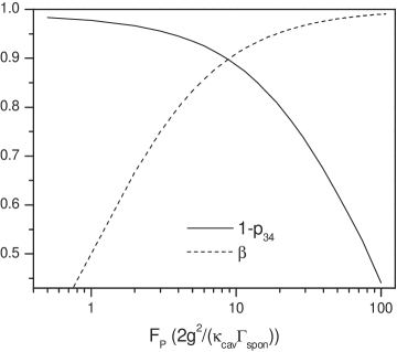
Figure 4: Dependence of indistinguishability and collection efficiency on the cavity-induced decay rate ($(F_{P}+1)\Gamma_{spon}$) of a quantum dot. Parameter values are: $\Gamma_{spon}=10^{9}~{}\textrm{s}^{-1}$, $\Gamma_{relax}=10^{11}~{}\textrm{s}^{-1}$, $\gamma_{deph}=0$, excitation laser is a Gaussian beam with a pulsewidth of $10^{-11}$ s. Peak laser Rabi frequency is changed between $1.1\times 10^{11}$ and $0.93\times 10^{11}~{}\textrm{s}^{-1}$.

We now study the dependence of indistinguishability, ($1-p_{34}$), on the cavity-induced decay rate ($(F_{P}+1)\Gamma_{spon}$) and dephasing. In Fig. 4, we plot the collection efficiency and indistinguishability as a function of the Purcell factor, $F_{P}$, for a quantum dot with $\gamma_{deph}=0$. We assume $\Gamma_{spon}=10^{9}~{}\textrm{s}^{-1}$ and $\Gamma_{relax}=10^{11}~{}\textrm{s}^{-1}$. Peak laser Rabi frequency is changed between $1.1\times 10^{11}$ and $0.93\times 10^{11}~{}\textrm{s}^{-1}$ in order to achieve $\pi$-pulse excitation for different Purcell factors. Collection efficiency is calculated by $\beta=F_{P}/(F_{P}+1)$, assuming that photons emitted to the cavity mode are collected with 100$\%$ efficiency. This assumption clearly constitutes an upper limit for the actual collection efficiency for typical microcavities Gérard et al. (2002).

Fig. 4 depicts one of the main results we present in this paper. Due to the time-jitter induced by the relaxation from the third level, there is a trade-off between collection efficiency and indistuingishability. For a Purcell factor of 100 we calculate a maximum indistuingishability of 44 $\%$ with a collection efficiency of 99 $\%$.

Figure 5: Dependence of indistinguishability and collection efficiency on dephasing ($\gamma_{deph}$). $\Gamma_{spon}=10^{9}~{}\textrm{s}^{-1}$, $F_{P}=9$, $\Gamma_{relax}=10^{11}~{}\textrm{s}^{-1}$, excitation laser is a Gaussian beam with a pulsewidth of $10^{-11}$ s. Peak laser Rabi frequency is $1.03\times 10^{11}~{}\textrm{s}^{-1}$ achieving $\pi$-pulse excitation.

The dependence of indistinguishability on dephasing is depicted in Fig. 5. As expected, dephasing has no effect on the collection efficiency. On the other hand, indistinguishability vanishes for $\gamma_{deph}>\Gamma_{spon}$. Since dephasing is effectively a non-referred quantum state measurement, it results in additional jitter in photon emission time.

To understand this effect, we should recall that dephasing of an optical transition is equivalent to a non-referred quantum state measurement that projects the emitter into either its excited or ground state. Reciprocal dephasing rate $\gamma_{deph}^{-1}$ then gives the average time interval between these state projections. In this case, photon emission is restricted to take place in between two subsequent measurement events, first (second) of which projects the emitter into the excited (ground) state. While the bandwidth of the emitted photon is then necessarily given by $\gamma_{deph}$ due to energy-time uncertainty, its emission (i.e. arrival) time will be randomly distributed within $\Gamma_{spon}^{-1}$. Since the information about the random emission times of any two photons is carried by the reservoir that causes the dephasing process, the photons will no longer be completely indistinguishable.

II.3 Quantum dot single photon source based on a cavity-assisted spin-flip Raman transition

Raman transition in a single three-level system strongly coupled to a high-Q cavity provides an alternative single photon generation scheme Law and Eberly (1996); Law and Kimble (1997); Kuhn et al. (1999). In contrast to the incoherently pumped source discussed in subsection II.2, this scheme realizes a coherently pumped single photon source that does not involve coupling to reservoirs other than the one into which single photons are emitted. It allows for pulse-shaping, and is suitable for quantum state transfer Cirac et al. (1997). In this part we discuss the application of this scheme to quantum dots, and demonstrate that arbitrarily high collection efficiency and indistinguishability can simultaneously be achieved in this scheme.

A quantum dot doped with a single conduction-band electron constitutes a three-level system in the $\Lambda$-configuration under constant magnetic fields along x-direction (Fig. 6) Imamoḡlu et al. (1999). Lowest energy conduction and valence band states of such a quantum dot are represented by $|m_{x}=\pm 1/2\rangle$ and $|m_{z}=\pm 3/2\rangle$ respectively due to the strong z-axis confinement, typical of quantum dots. The magnetic field results in the Zeeman splitting of the spin up ($|m_{x}=1/2\rangle$) and down ($|m_{x}=-1/2\rangle$) levels in the conduction band. Considering an electron g-factor of 2 and an applied field of 10 Tesla which is available from typical magneto-optical cryostats, the splitting is expected to be $\sim$1 meV. At cryogenic temperatures, this splitting is much larger than other broadenings in consideration, thus a three-level system in the $\Lambda$-configuration is obtained. We emphasize that none of the experimental measurements carried out on self-assembled quantum dots yield any signatures of Auger recombination processes for trion (2 electron and one hole system) or biexciton transitions. In particular, lifetime measurements carried out on biexcitons gave $\tau_{biexc}\sim\tau_{exc}/1.5$, indicating the absence of Auger enhancement of biexciton decay Kiraz et al. (2002).

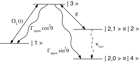
Figure 6: Single photon source based on cavity-assisted spin-flip Raman transition in a single quantum dot. Dashed line demonstrates the generated single photons via cavity leakage.

We assume that an x-polarized laser pulse is applied resonantly between levels $|m_{x}=1/2\rangle$ and $|m_{z}=3/2\rangle$ (or $|m_{z}=-3/2\rangle$) while levels $|m_{x}=-1/2\rangle$ and $|m_{z}=3/2\rangle$ (or $|m_{z}=-3/2\rangle$) are strongly coupled via a resonant y-polarized cavity mode. Considering the number of cavity photons to be limited to 0 and 1, the electronic energy level $|m_{x}=-1/2\rangle$, can be represented by the levels $|m_{x}=-1/2,1\rangle$ and $|m_{x}=-1/2,0\rangle$ corresponding to 1 and 0 cavity photon respectively. We will abbreviate the energy levels $|m_{x}=1/2\rangle$, $|m_{z}=3/2\rangle$, $|m_{x}=-1/2,1\rangle$, and $|m_{x}=-1/2,0\rangle$ as $|1\rangle$, $|2\rangle$, $|3\rangle$, and $|4\rangle$ respectively.

In such a three-level system, Raman transition induced by the laser and cavity fields together with the finite cavity leakage rate, $\kappa_{cav}$, enable the generation of a single cavity photon per pulse. For large field couplings, level $|3\rangle$ can be totally bypassed resulting in ideal coherent population transfer between levels $|1\rangle$ and $|2\rangle$. This single photon source has therefore the potential to achieve 100$\%$ collection efficiency together with ideal two-photon interference. This scheme is to a large extent insensitive to quantum dot size fluctuations and may enable the use of different quantum dots in simultaneous generation of indistinguishable photons, provided that the cavity resonances and the electron g-factors are identical. Variations in the electron g-factor between different quantum dots would limit the photon indistinguishability due to spectral mismatch between the generated photons: We do not consider this potential limitation in this paper. In general, spontaneous emission and dephasing in $|3\rangle$-$|2\rangle$ transition are the principal sources of non-ideal two-photon interference and decreased collection efficiency in this scheme. The ultimate limit for photon indistinguishability due to jitter in emission time is given by spin decoherence of the ground state.

Such a single photon source has been recently demonstrated using single cold atoms trapped in a high-Q Fabry-Perot cavity Kuhn et al. (2002). Due to the limited trapping times, at most only 7 photons were emitted by a single atom in this demonstration. Practical realizations of this scheme also require a means to bring the system from level $|4\rangle$ to $|1\rangle$ at the end of each single photon generation event. In Ref. Kuhn et al. (2002) this was achieved by a recycling laser pulse. The applied recycling laser pulse determines the end of the single-photon pulse and can in principle limit the collection efficiency for systems with long spontaneous emission lifetimes. In the case of quantum dots, recycling can be achieved by a similar laser pulse applied between levels $|4\rangle$ and $|3\rangle$. An alternative recycling mechanism can be the application of a Raman $\pi$-pulse, generated by two detuned laser pulses satisfying the Raman resonance condition between levels $|4\rangle$ and $|1\rangle$.

We now discuss the numerical analysis of this system which is described by the interaction Hamiltonian

$$\hat{H}_{int}=i\hbar g(\hat{\sigma}_{32}-\hat{\sigma}_{23})+i\hbar\Omega_{L}(\hat{\sigma}_{31}-\hat{\sigma}_{13})\,.$$ (30)

We use the master equation

$$\frac{d}{dt}\hat{\rho} = \frac{1}{i\hbar}\left[\hat{H}_{int},\hat{\rho}\right]+\kappa_{cav}\left(2\hat{\sigma}_{42}\hat{\rho}\hat{\sigma}_{24}-\hat{\sigma}_{22}\hat{\rho}-\hat{\rho}\hat{\sigma}_{22}\right)$$ (31)

$$+\frac{\Gamma_{spon}\cos^{2}\theta}{2}\left(2\hat{\sigma}_{13}\hat{\rho}\hat{\sigma}_{31}-\hat{\sigma}_{33}\hat{\rho}-\hat{\rho}\hat{\sigma}_{33}\right)$$

$$+\frac{\Gamma_{spon}\sin^{2}\theta}{2}\left(2\hat{\sigma}_{43}\hat{\rho}\hat{\sigma}_{34}-\hat{\sigma}_{33}\hat{\rho}-\hat{\rho}\hat{\sigma}_{33}\right)\,,$$

to derive the optical Bloch equations. In the presence of dephasing caused by reservoirs other than the radiation field ($\gamma_{deph}$), we define the total coherence decay rate in transitions from level $|3\rangle$ as $\gamma=\frac{\Gamma_{spon}}{2}+\gamma_{deph}$. Branching of spontaneous emission from level $|3\rangle$ to levels $|1\rangle$ and $|4\rangle$ is indicated by $\cos^{2}\theta$ and $\sin^{2}\theta$, respectively, as shown in Fig. 6.

$\widetilde{G}^{(1)}(t,\tau)=\langle\hat{\sigma}_{24}(t+\tau)\hat{\sigma}_{42}(t)\rangle$ is calculated by applying the quantum regression theorem to the optical Bloch equations for $\hat{\sigma}_{14}$, $\hat{\sigma}_{24}$, and $\hat{\sigma}_{34}$. The following set of differential equations are then obtained

$$\frac{d}{d\tau}F(t,\tau) = -\Omega_{L}(t)H(t,\tau)\,,$$

$$\frac{d}{d\tau}\widetilde{G}^{(1)}(t,\tau) = -gH(t,\tau)-\kappa_{cav}\widetilde{G}^{(1)}(t,\tau)\,,$$ (32)

$$\frac{d}{d\tau}H(t,\tau) = \Omega_{L}(t)F(t,\tau)+g\widetilde{G}^{(1)}(t,\tau)-\gamma H(t,\tau)\,.$$

The variables: $\widetilde{G}^{(1)}(t,\tau)=\langle\hat{\sigma}_{24}(t+\tau)\hat{\sigma}_{42}(t)\rangle$, $F(t,\tau)=\langle\hat{\sigma}_{14}(t+\tau)\hat{\sigma}_{42}(t)\rangle$, and $H(t,\tau)=\langle\hat{\sigma}_{34}(t+\tau)\hat{\sigma}_{42}(t)\rangle$ have initial conditions $\widetilde{G}^{(1)}(t,0)=\langle\hat{\sigma}_{22}(t)\rangle$, $F(t,0)=\langle\hat{\sigma}_{12}(t)\rangle$, and $H(t,0)=\langle\hat{\sigma}_{32}(t)\rangle$.

Following the solutions of the optical Bloch equations and the set of Eqs. (32), normalized coincidence detection probability, $p_{34}$, is calculated using Eq. (25) as described in section II.1. Assuming ideal detection of the photons emitted to the cavity mode, we calculate the collection efficiency by the number of photons emitted from the cavity

$$n=2\kappa_{cav}\int_{0}^{\infty}\langle\hat{\sigma}_{22}(t)\rangle\,dt\,.$$ (33)

Our principal numerical results are depicted in Fig. 7 where we consider a dephasing-free system, and analyze the dependence of the collection efficiency and indistinguishability on the cavity coupling. In these calculations we assume a potential quantum dot cavity-QED system with relatively small cavity decay rate of $\kappa_{cav}=10\Gamma_{spon}$ Kiraz et al. (2003). Laser pulse is chosen to be Gaussian with a constant pulsewidth. The peak laser Rabi frequency is increased with increased cavity coupling in order to reach the onset of saturation in the emitted number of photons. The large pulsewidth of 10 ensures the operation in the regime where collection efficiency and indistinguishability are independent of the pulsewidth. All other parameters are kept constant at their values noted in the figure caption. We choose both spontaneous emission channels to be equally present ($\theta=\pi/4$).

Figure 7: Dependence of indistinguishability and collection efficiency on cavity coupling. Parameter values are: $\Gamma_{spon}=1$, $\kappa_{cav}=10$, $\gamma_{deph}=0$, $\theta=\pi/4$, a Gaussian pulse with pulsewidth=10, peak laser Rabi frequency is changed between 0.75 and 2.8 . Inset: Dependence of indistinguishability and collection efficiency on $\kappa_{cav}$ for a constant $F_{P}$ of 20. Parameter values are: $\Gamma_{spon}=1$, $\gamma_{deph}=0$, $\theta=\pi/4$, laser pulsewidth of $10/\Gamma_{spon}$, peak laser Rabi frequency of 1.9 - 2.1 .

In contrast to the incoherently pumped single photon source, Fig. 7 shows that arbitrarily high indistinguishability and collection efficiency can simultaneously be achieved with better cavity coupling using this scheme. For a cavity coupling that corresponds to a Purcell factor of 40 ($F_{P}=2g^{2}/(\kappa_{cav}\Gamma_{spon})=40$), our calculations reveal 99 $\%$ indistinguishability together with 99 $\%$ collection efficiency. This regime of operation is readily available in current state-of-the-art experiments with atoms Hood et al. (2000). While such a Purcell factor has not been observed for solid-state emitters in microcavity structures to date, recent theoretical Vuckovic and Yamamoto (2003) and experimental Kiraz et al. (2003); Akahane et al. (2003) progress indicate that the aforementioned values could be well within reach.

As expected, the dependence of $\beta$ on cavity coupling is exactly given by $2F_{P}/(1+2F_{P})$. This is due to the spontaneous emission from level $|3\rangle$ to $|4\rangle$, namely $\Gamma_{spon}\sin^{2}\theta=\Gamma_{spon}/2$, which defines the relevant Purcell factor. As shown in the inset in Fig. 7, our calculations considering different $\kappa_{cav}$ values for a constant Purcell factor revealed similar collection efficiency and indistinguishablity values. Hence Purcell factor is the most important parameter in determining the characteristics of this single photon source.

Achieving the regime of large indistinguishability and collection efficiency together with small laser pulsewidths is also highly desirable for efficient quantum information processing applications. In this single photon source that relies on cavity-assisted Raman transition, lower limits for the laser pulsewidth are in general given by the inverse cavity coupling constant ($g^{-1}$) and cavity decay rate ($\kappa_{cav}^{-1}$) Kuhn et al. (1999). We analyze the effect of the laser pulsewidth to indistinguishability and collection efficiency in Fig. 8. In this figure we consider the potential quantum dot cavity-QED system analyzed in Fig. 7 ($\kappa_{cav}=10\Gamma_{spon}$) while assuming a Purcell factor of 20 ($g=10\Gamma_{spon}$). As in the previous cases, we change the maximum laser Rabi frequency for different pulsewidth values in order to reach the onset of saturation. For this system, we conclude that a minimum pulsewidth of $1/\Gamma_{spon}$ is sufficient to achieve maximum indistinguishability and collection efficiency.

Figure 8: Dependence of indistinguishability and collection efficiency on the Gaussian laser pulsewidth. Parameter values are: $\Gamma_{spon}=1$, $g=10$, $\kappa_{cav}=10$ ($F_{P}=20$), $\gamma_{deph}=0$, $\theta=\pi/4$. Peak laser Rabi frequency is changed between 2.1 and 10.5 .

The two spontaneous emission channels from level $|3\rangle$ have complementary effects on collection efficiency and indistinguishability. Spontaneous emission from level $|3\rangle$ to $|1\rangle$ reduces indistinguishability while having no effect on collection efficiency. This spontaneous emission channel, $\Gamma_{spon}\cos^{2}\theta$, effectively represents a time-jitter mechanism for single photon generation. In contrast, spontaneous emission from level $|3\rangle$ to level $|4\rangle$ has no effect on indistinguishability while reducing collection efficiency. These effects are clearly demonstrated in Fig. 9 where we plot the dependence of collection efficiency and indistinguishability on $\theta$.

Figure 9: Dependence of indistinguishability and collection efficiency on $\theta$. Parameter values are: $\Gamma_{spon}=1$, $g=10$, $\kappa_{cav}=10$ ($F_{P}=20$), $\gamma_{deph}=0$, $\theta=\pi/4$. A Gaussian pulse is assumed with pulsewidth=1 and peak Rabi frequency of 6.2 .

Finally in Fig. 10 we analyze the dependence of indistiguishability and collection efficiency on dephasing of transitions from level $|3\rangle$. In contrast to the case of an incoherently pumped quantum dot (Fig. 5), there is a small but non-zero dependence of collection effciency on dephasing. For the parameters we chose, collection efficiencies of 0.975 and 0.970 were calculated for dephasing rates of $0$ and $1.5\Gamma_{spon}$ respectively.

Figure 10: Dependence of indistinguishability and collection efficiency on the dephasing rate. Parameter values are: $\Gamma_{spon}=1$, $g=10$, $\kappa_{cav}=10$ ($F_{P}=20$), $\theta=\pi/4$, a Gaussian laser pulse is assumed with pulsewidth=1 and peak Rabi frequency of 6.2 .

III Indistinguishability and nondeterministic linear-optics gates

Having determined the limits and dependence of photon collection efficiency and indistinguishability on system configuration and cavity parameters, we turn to the issue of photon distinguishability effects on the performance of LOQC gates. Related question of dependence on photon loss Knill et al. (2001); Lund et al. (2003) and detection inefficiency Glancy et al. (2002) have previously been analyzed. For semiconductor single photon sources, photon loss can be minimized by increasing collection efficiency, in principle, to near unity value. Therefore, close to ideal photon emission can be achieved with better cavity designs and coupling. However, as we have shown in previous sections, an incoherently pumped semiconductor photon source suffers heavily from emission time-jitter, especially for large values of Purcell factor, while a semiconductor system based on cavity-assisted spin-flip Raman transition shows promise for near unity collection efficiency and indistinguishability. To assess the cavity requirements for the latter system, we analyze the reduction in gate fidelity arising from photon emission time-jitter in a linear optics controlled phase gate, a key element for most quantum gate constructions.

This non-deterministic gate operates as follows: Given a two-mode input state of the form

$$|\Psi_{\rm in}\rangle=\bigl{[}\alpha|00\rangle+\beta|01\rangle+\delta|10\rangle+\gamma|11\rangle\bigr{]}\,,$$ (34)

where $|\alpha|^{2}+|\beta|^{2}+|\gamma|^{2}+|\delta|^{2}=1$, the state at the two output modes transforms into

$$|\Psi_{\rm out}\rangle=\bigl{[}\alpha|00\rangle+\beta|01\rangle+\delta|10\rangle+e^{\rm{i}\Phi}\gamma|11\rangle\ \bigr{]}\,,$$ (35)

with a certain probability of success, $|p|^{2}$. A realization of such a gate using all linear optical elements, two helper single photons on demand, and two photon-number resolving single-photon detectors is depicted in Fig. 11 for the special case of $\Phi=\pi$ Knill (2001, 2002). This realization consists of two input modes for the incoming quantum state to be transformed and two ancilla modes with a single helper photon in each mode. After four beam splitters with settings $\theta_{1}=\theta_{2}=-\theta_{3}=54.74^{\circ}$ and $\theta_{4}=17.63^{\circ}$, postselection is performed via photon-number measurements on output modes 3 and 4. Conditional to single-photon detection in each of these modes, the quantum state in Eq. (34) is transformed into Eq. (35). The probability of success for this construction is $2/27$, which is slightly better then $1/16$, the probability of success of the original proposal using only one helper photon with two ancilla modes Knill et al. (2001).

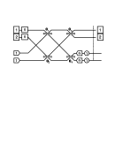
Figure 11: Optical network realizing CS${}_{180^{\circ}}$.

This is the probability of success for ideal systems comprising indistinguishable photons, and unity efficiency number resolving single photon detectors. We now proceed to investigate the effects of photon distinguishability arising from physical constraints of the single photon sources in consideration. In the presence of a temporal jitter, $\epsilon$, in the photon emission time, a single photon state can be represented as

$$|1\rangle=\int\rm{d}\omega f(\omega)e^{\rm{i}\omega\epsilon}a_{j}^{\dagger}(\omega)|0\rangle\,,$$ (36)

where $f(\omega)$ is the spectrum of the photon wave-packet. For photons from a quantum dot in a cavity, the function $f(\omega)$ is a Lorentzian yielding a double-sided exponential dip in the Hong-Ou-Mandel interference Hong et al. (1987). In the presence of relative time jitter, the visibility of interference is obtained after ensemble averaging over the time-jitter $\epsilon$ in the range $[0,\epsilon_{0}]$ yielding the relation

$$V(\epsilon_{0})=\frac{1}{\epsilon_{0}/\tau}(1-\text{e}^{-\epsilon_{0}/\tau})\,,$$ (37)

for a uniform distribution. In order to analyze time-jitter effects on the fidelity of the quantum gate shown in Fig. 11, we introduce a time-jitter for the helper photon in mode 4. For clarity, we keep the remaining photons in other modes ideal and indistinguishable. The symmetry of the gate ensures that each introduced time-jitter adds to the power dependence of the overall error.

Rewriting Eq. (36) as

$$|1\rangle=\int\rm{d}\omega f(\omega)[1-(1-e^{\rm{i}\omega\epsilon})]c_{j}^{\dagger}(\omega)|0\rangle\,,$$ (38)

allows us to represent the output state in terms of the ideal output state and the time-jitter dependent part $|\Phi(\epsilon)\rangle$:

$$|\overline{\Psi}_{\rm out}\rangle=|\Psi_{\rm out}\rangle-|\Phi(\epsilon)\rangle\,.$$ (39)

Using the definition of the gate fidelity for a particular $|\overline{\Psi}_{\rm out}\rangle$

$$F_{|\overline{\Psi}_{\rm out}\rangle}=\frac{|\langle\Psi_{\rm out}|\overline{\Psi}_{\rm out}\rangle|^{2}}{\langle\Psi_{\rm out}|\Psi_{\rm out}\rangle\langle\overline{\Psi}_{\rm out}|\overline{\Psi}_{\rm out}\rangle}\,,$$ (40)

with Eq. 39 we obtain

$$F_{|\overline{\Psi}_{\rm out}\rangle}=\frac{|p|^{2}-2\rm{Re}\left[{\langle\Psi_{\rm out}|\Phi(\epsilon)\rangle}\right]+\frac{|\langle\Psi_{\rm out}|\Phi(\epsilon)\rangle|^{2}}{|p|^{2}}}{|p|^{2}-2\rm{Re}\left[{\langle\Psi_{\rm out}|\Phi(\epsilon)\rangle}\right]+\langle\Phi(\epsilon)|\Phi(\epsilon)\rangle}\,,$$ (41)

where $|p|^{2}=\langle\Psi_{\rm out}|\Psi_{\rm out}\rangle$. Given the particular realization of this gate as depicted in Fig. 11, the overall gate fidelity takes the form

$$F=\text{min}\left[\bigl{<}F_{|\overline{\Psi}_{\rm out}\rangle}\bigr{>}_{\epsilon}^{\epsilon_{0}}\right]=\frac{c_{0}+c_{1}V(\epsilon_{0})+c_{2}V^{2}(\epsilon_{0})}{d_{0}+d_{1}V(\epsilon_{0})+d_{2}V^{2}(\epsilon_{0})}\,,$$ (42)

where $\langle\cdot\rangle_{\epsilon}^{\epsilon_{0}}$ denotes ensemble averaging over time-jitter $\epsilon$ in the range $[0,\,\epsilon_{0}]$ using an appropriate weight function and $V(\epsilon_{0})$ is the degree of indistinguishability, or the corresponding visibility in a Hong-Ou-Mandel interference. The coefficients $c_{i}$ and $d_{i}$ in Eq. (42) depend not only on the gate properties such as the probability of success, but also on the initial input state through the coefficients $\alpha$, $\beta$, and $\gamma$. Consequently, the gate fidelity becomes a function of the properties of the initial input state.

A plot for minimum gate fidelity (corresponding to a $|11\rangle$ input state) found after extensive search over a set of initial input states is shown in Fig. 12 as a function of time-jitter normalized to photon pulsewidth $(\epsilon_{0}/\tau)$. As is evident from the graph, time-jitter on the order of 0.3% is the limiting case in order to achieve fidelity of 99%. For an incoherently pumped quantum dot single photon source as analyzed in section II.2, the emission time-jitter is on the order of $1\times 10^{-11}$ s. Thus, for single photon pulsewidth on the order of $1\times 10^{-9}$ s, this fidelity threshold cannot be satisfied. As is also clear from Fig. 4, this corresponds to a Purcell factor of order unity and collection efficiency of about 50%. In a cavity-assisted spin-flip Raman transition, however, indistinguishability and collection efficiency are both shown to increase in Fig. 7 as the Purcell factor increases. This, in turn, casts a single constraint on the cavity quality factor, requiring $F_{P}\geq 40$, in order to achieve both indistinguishability and collection efficiency required for gate operations for LOQC. This threshold for cavity quality factor is within the realistic values to date. We emphasize that so far there has been no calculation on the maximum allowed time-jitter error for LOQC scheme Knill et al. (2001).

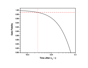
Figure 12: Dependence of nonlinear sign gate fidelity $F$, on normalized time-jitter $\epsilon$. The horizontal line indicates the 99% fidelity threshold. The vertical line indicates tolerable time-jitter threshold.

IV Conclusions

We analyzed the effects of cavity coupling, spontaneous emission rate, dephasing, and laser pulsewidth on indistinguishability and collection efficiency for two distinct types of single photon sources based on two and three-level emitters. We showed that, in contrast to incoherently pumped systems, a single photon source based on cavity-assisted spin-flip Raman transition has the potential to simultaneously achieve high levels of indistinguishability and collection efficiency. For this system, in the absence of dephasing, 99 $\%$ indistinguishability and collection efficiency are achieved for a Purcell factor of 40. Our analysis revealed that strong coupling regime of cavity-QED ($g>\{\gamma,\kappa_{cav}\}$) is not a requirement for optimum operation while, in the presence of dephasing, the characteristics of the system is determined by $g^{2}/\kappa_{cav}\gamma_{deph}$ rather than the Purcell factor. The desired regime of operation, i.e. Purcell factor of 40 in the absence of dephasing, is readily available for atoms in high-Q Fabry-Perot cavities. It is also within the reach for solid-state based single photon sources embedded in microcavity structures given current technology. We also analyzed the reduction in gate fidelity arising from photon emission-time-jitter in a linear optics controlled sign gate. We found that the aforementioned Purcell regime provides gate performance with error $<\,1\%$ using the single photon source based on cavity-assisted Raman transition.