Bipartite entanglement and localization of one-particle states

Abstract

We study bipartite entanglement in a general one-particle state, and find that the linear entropy, quantifying the bipartite entanglement, is directly connected to the paricitpation ratio, charaterizing the state localization. The more extended the state is, the more entangled the state. We apply the general formalism to investigate ground-state and dynamical properties of entanglement in the one-dimensional Harper model.

Entanglement is a unique phenomenon of quantum systems that does not exist classically. It has attracted more interest due to its potential applications in quantum communication and information processing Nie00 such as quantum teleportation Ben1 , superdense coding Ben2 , quantum key distribution Ekert , and telecoloning Mur . On the other hand, entanglement has been proved to be playing an important role in condensed matter physics. There are many studies on entanglement in the Heisenberg spin models Heisen1 ; Heisen2 ; Wang1 , Ising models in a transverse magnetic field Connor ; Gun , and related itinerant fermionic systems Fermion . In the context of quantum phase transition, entanglment is also an indicator of the transition which can not be captured by common statistical physics Osb ; Ost .

Recently, pairwise entanglement sharing in one-particle states was studied Lak03 using the concurrence Conc in the Harper model Harper . Here, we study another type of entanglement of one-particle states, the bipartite entanglement, which refers to entanglement between two subsystems when a whole system is divided into two parts. We reveal that the average bipartite entanglement directly connects to state localization.

The one-particle states permeate many physics systems. For examples, for one electron moving on a substrate potential, the eigenfunctins are one-particle states. In quantum spin chain models with only one spin up (down) and all other spins down (up), the eigenfuntions of the model are one-magnon states.

We consider a system containing $N$ two-level systems (qubits) with $|0\rangle$ being the excited state and $|1\rangle$ the ground state. A general one-particle state is then written as

$$|\Psi\rangle= \psi_{1}|1000\ldots 0\rangle+\psi_{2}|0100\ldots 0\rangle$$

$$+\ldots+\psi_{N}|0000\ldots 1\rangle$$ (1)

Here, $\{|\psi_{n}|^{2}\}$ is a probability distribution, satisfying the normalization condition $\sum_{n=1}^{N}|\psi_{n}|^{2}=1.$ When $|\psi_{n}|=1/\sqrt{N}$, state $|\Psi\rangle$ reduces to the W state W ; Wang1 , one representative state in quantum information theory.

We now consider bipartite entanglement between a block of $L$ qubits and the rest $N-L$ qubits. Bipartite entanglement of a pure state can be measured by the linear entropy of reduced density matrices Ben3 .

$$E(|\Psi\rangle)=1-\text{Tr}(\rho_{i}),\quad i\in\{1,2\}$$ (2)

where $\rho_{i}$ is the reduced density matrix for subsystem $i$.

To calcualte bipartite entanglement, we first consider a simple situation, namely, the entanglement between the first qubit and the rest $N-1$ qubits. The one-particle state can be written in the following form:

$$|\Psi\rangle=\psi_{1}|1\rangle\otimes|\alpha\rangle+\sqrt{\sum_{n=2}^{N}|\psi_{n}|^{2}}|0\rangle\otimes|\beta\rangle$$ (3)

where

$$|\alpha\rangle= |00\ldots 0\rangle,$$

$$|\beta\rangle= \frac{1}{\sqrt{\sum_{n=2}^{N}|\psi_{n}|^{2}}}(\psi_{2}|100\ldots 0\rangle+\psi_{3}|010\ldots 0\rangle$$

$$+\ldots+\psi_{N}|00\ldots 1\rangle)$$ (4)

are two orthonormal states of $N-1$ qubits. Then the reduced density matrix for qubit 1 is easily found to be

$$\rho_{1}=\left(\begin{array}[]{cc}1-|\psi_{1}|^{2}&0\\ 0&|\psi_{1}|^{2}\end{array}\right)$$ (5)

in the basis $\{|0\rangle,|1\rangle\}$. Therefore, from Eqs. (2) and (5), the linear entropy of qubit 1 is obtained as $E_{1,N-1}^{(1)}=2(|\psi_{1}|^{2}-|\psi_{1}|^{4}),$ where the superscript denotes the first qubit. In the same way, we may find the linear entropy for the $n$-th qubit as

$$E_{1,N-1}^{(n)}=2(|\psi_{n}|^{2}-|\psi_{n}|^{4}),$$ (6)

quantifying the degree of bipartite entanglement between $n$-th qubit and the rest.

Making an average of entanglement over all qubits, we obtain

$$E_{1,N-1}=\langle E_{1,N-1}^{(n)}\rangle= \frac{2}{N}\sum_{n=1}^{N}(|\psi_{n}|^{2}-|\psi_{n}|^{4})$$

$$= \frac{2}{N}\left(1-\sum_{n=1}^{N}|\psi_{n}|^{4}\right)=\frac{2}{N}E_{s},$$ (7)

where $E_{s}=(1-\sum_{n=1}^{N}|\psi_{n}|^{4})$ is the quantum state linear entropy Georgeot00 for state $|\Psi\rangle$.

We now consider more general situations, namely, the bipartite entanglement between a block of $L$ qubits and the rest of the system. We pick up $L$ qubits $\{1^{{\prime}},2^{{\prime}},\ldots,L^{{\prime}}\}$ from $N$ qubits, and there are totally $C_{N}^{L}$ options. In the same way as above, we can calculate the linear entropy of $L$ qubits as

$$E_{L,N-L}^{\{1^{\prime},\ldots,L^{\prime}\}}=2(|\psi_{1^{{\prime}}}|^{2}+\ldots+|\psi_{L^{{}^{\prime}}}|^{2})-2(|\psi_{1^{{\prime}}}|^{2}+\ldots+|\psi_{L^{{}^{\prime}}}|^{2})^{2}.$$ (8)

Now, we make an average of the linear entropy $E_{L,N-L}^{\{1^{\prime},\ldots,L^{\prime}\}}$ over the $C_{N}^{L}$ options. Formally, the average entropy is given by

$$E_{L,N-L}= \langle E_{L,N-L}^{\{1^{\prime},\ldots,L^{\prime}\}}\rangle=\Big{[}\sum_{\{1^{\prime},\ldots,L^{\prime}\}}\frac{2}{C_{N}^{L}}(|\psi_{1^{{\prime}}}|^{2}+\ldots+|\psi_{L^{{}^{\prime}}}|^{2})$$

$$- \frac{2}{C_{N}^{L}}(|\psi_{1^{{\prime}}}|^{2}+\ldots+|\psi_{L^{{}^{\prime}}}|^{2})^{2}\Big{]}.$$ (9)

The first term in the summation of the above equation can be easily evaluated as

$$\frac{2}{C_{N}^{L}}\sum_{\{1^{\prime},\ldots,L^{\prime}\}}(|\psi_{1^{{\prime}}}|^{2}+|\psi_{2^{{\prime}}}|^{2}+\ldots+|\psi_{L^{{\prime}}}|^{2})=\frac{2L}{N}.$$ (10)

Next, we evaluate the second term of the summation in Eq. (9). The following relation

$$\sum_{n>m}2|\psi_{n}|^{2}|\psi_{m}|^{2}=1-\sum_{n=1}^{N}|\psi_{n}|^{4}.$$ (11)

is useful, resulting from the normalization condition of state $|\Psi\rangle$. Note that the summation on the left hand of the above equation contains $C_{N}^{2}$ terms. By applying the above relation, the second term of the summation in Eq. (9) is obtained as

$$-\frac{2L}{N}\sum_{n=1}^{N}|\psi_{n}|^{4}-\frac{2C_{L}^{2}}{C_{N}^{2}}\left(1-\sum_{n=1}^{N}|\psi_{n}|^{4}\right).$$ (12)

Substituting Eqs. (10) and (12) to Eq. (9) leads to

$$E_{L,N-L}=2\left(\frac{L}{N}-\frac{C_{L}^{2}}{C_{N}^{2}}\right)E_{s}=\frac{2L(N-L)}{N(N-1)}E_{s}.$$ (13)

As we expected, the average linear entropy is invariant under the transformation $L\rightarrow N-L$.

The above result (13) shows that the average bipartite entanglement between a block of $L$ qubits and the rest $N-L$ qubits is proportional to the quantum state linear entropy $E_{s}$. For the W state, the quantum state linear entropy $E_{s}=1-1/N$, and thus the average linear entropy becomes

$$E_{L,N-L}=2L(N-L)/N^{2}.$$ (14)

If $N$ is even being fixed and $L=N/2$, the linear entropy $E_{L,N-L}=1/2$ becomes maximal, equal to the amount of bipartite entanglement of a Bell state.

There exists a close relation between the average pairwise entanglement and state localization for one-particle states as discussed in Ref. Lak03 . We now study relations between bipartite entanglement and state localization. The degree of localization can be studied by a simple quantity, the participation ratio defined by

$$p=\frac{1}{N\sum_{n=1}^{N}|\psi_{n}|^{4}}.$$ (15)

Then, from the above equation, the quantum state linear entropy can be written as

$$E_{s}=1-\frac{1}{Np}.$$ (16)

Subsitituting Eq. (16) to Eq. (13) leads to

$$E_{L,N-L}=\frac{2L(N-L)}{N(N-1)}\left(1-\frac{1}{Np}\right),$$ (17)

which builds a direct connection between bipartite entanglement and state localization. It is evident that the larger $p$ is, the larger the linear entropy. In other words, the more extended the one-particle state is, the more entangled the state.

In a recent relevant work BambiLiWang1 , we find that there is a relation between the average square of concurrence and the participation ratio given by

$$\langle C^{2}\rangle=\frac{4}{N(N-1)}\left(1-\frac{1}{Np}\right).$$ (18)

Then, from Eqs. (17) and (18), we obtain a connection between bipartite entanglement and pairwise entanglement given by

$$E_{L,N-L}=\frac{L(N-L)}{2}\langle C^{2}\rangle.$$ (19)

Therefore, for one-particle state, the average linear entropy, the average square of concurence, and the participation ratio are interrelated together by simple relations. Next, we consider an example of one-particle states, and study quantum entanglement and its relations to state localization induced by on-site potentials in the quasiperiodic one-dimensional Harper model Harper .

The Hamiltonian describing electrons hopping in a one-dimentional lattice can be written as Harper

$$H=\sum_{n=1}^{N}\frac{1}{2}(c_{n}^{\dagger}c_{n+1}+c_{n+1}^{\dagger}c_{n})+V_{n}c_{n}^{\dagger}c_{n},$$ (20)

where $c_{n}^{\dagger}$ and $c_{n}$ are the creation and annihilation operators, respectively, and $V_{n}$ is the on-site potential. This Hamiltonian describes electrons moving on a substrate potential. The different forms of on-site potential $V_{n}$ lead to different behaviors of electrons.

For the Harper model, the on-site potential is given by

$$V_{n}=\lambda\cos(2\pi n\sigma)$$ (21)

where $\sigma$ determines the period of potential and $\lambda$ is the amplitude of the potential. It is well known that the dynamics of the Harper model is characterized by parameter $\lambda$ Gei . If $\lambda<1,$ the electron is in a quasiballistic extended state, but in a localized state when $\lambda>1.$ The critical Harper model corresponds to $\lambda=1$, where the spectrum is a Cantor set.

We consider one-electron states in the Harper model. For studying entanglement in this fermionic system, we adopt the approach given in Ref. Fermion , namely, we first mapping electronic states to qubit states and study entanglement of fermions by calculating entanglement of qubits. After the mapping, the one-particle wavefunction of Harper model can be formally written in the form of a general state given by Eq. (1). Then, we may apply the general result (13) to calculate bipartite entanglement.

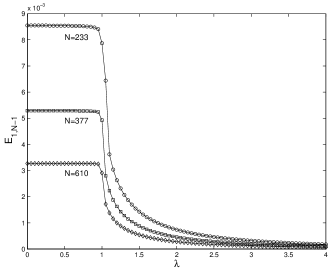
Figure 1: The average linear entropy as a function of $\lambda$ for differnet lengths of the chain. The parameter $\sigma$ is $F(n-1)/F(n)$ with $F(n)=N$, where $\{F(n)\}$ is the Fibonacci sequence.

For convenience, we examine the average bipartite entanglment between one local fermionic mode (LFM) and the rest for the ground state of the system. The LFMs refer to sites which can be either empty or occupied by an electron Bravyi . Figure 1 gives results of the linear entropy for different lengths of system. We notice that when the amplitude of the on-site potential increases but does not reach the value $\lambda=1$, the average entanglement $E_{1,N-1}$ is almost keeping a constant value, varying a very little bit. The entanglement is not destroyed by the external potential in this region. However, when $\lambda=1$, $E_{1,N-1}$ has a sudden jump down to a value close to zero. For larger $\lambda$, the ground state is almost not entangled. In Fig. 1, we also observe that the maximal value of the averge linear entropy decreases by increasing the length of the system, which agrees with the analytical results. Moreover, we make numerical caculations of the ground-state linear entropy $E_{s}$, and the results show a critical behavior around $\lambda=1$, which confirms the relation (13).

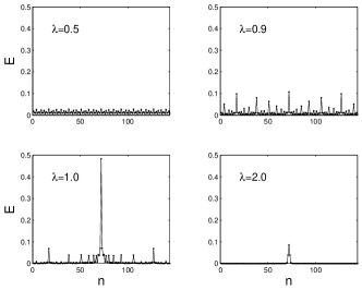
Figure 2: The distribution of the linear entropy for different $\lambda$ with $N=144$ and $\sigma=89/144$.

To understand the underlying mechanism of the transition of entanglment induced by the change of on-site potential, we study the distribution of the linear entropy $E_{1,N-1}^{(n)}$. If the on-site potential is absent, the entanglment distributes evenly on the lattice sites. Figure 2 shows the distribution of the linear entropy for different $\lambda$. When $\lambda=0.5$ smaller than $\lambda_{c}$, the entanglment is almost even. When $\lambda=0.9$ near to $\lambda_{c}$, the uneven distribution becomes distinct but the state is still not localized. When $\lambda=\lambda_{c}$, a significant change takes place, and a large peak of entanglement appears at the center of the lattice and the entanglement at most of the other sites are suppressed. The entanglement between the LFM at the center and the rest becomes dominant. The ground state is localized by the effects of on-site potential $V_{n}$ in this case. When $\lambda=2$ larger than $\lambda_{c}$, the entanglment at most sites is suppressed to zero except a few sites near the center of lattice is still of finite value, although they are also suppressed. Thus, the localization is enhanced when the amplitude of the potential increases. Further more, the biparticle entanglment between a block of LFMs and the rest for such a one-particle state are also calculated and shows similar behaviors as the linear entropy $E_{1,N-1}$.

Having studied ground-state entanglement of the Harper model, we now examine dynamics of entanglement. The time evolution can be described by the following time-dependent equation

$$i\frac{d\psi_{n}}{dt}=\frac{1}{2}(\psi_{n+1}+\psi_{n-1})+\lambda\cos(2\pi n\sigma).$$ (22)

The wave packet is localized initially at the center of the chain and the above equation can be solved numerically by integration. In our calculations, we adopt the periodic boundary condition. The variance of the wave packet

$$\sigma^{2}(t)=\sum_{n=1}^{N}(n-\bar{n})^{2}|\psi_{n}(t)|^{2}$$ (23)

is studied in Ref. Gei and different time evolution behaviors were shown.

When the state vectors at any time are obtained by integration, we can calculate bipartite entanglment between the block of LFMs and the rest of chain. In Fig. 3, we plot the average entanglment $E_{1,N-1}$ for several value of $\lambda$. When $\lambda<\lambda_{c},$ $E_{1,N-1}$ exhbits a rapid initial increase, which corresponds to the variance $\sigma^{2}(t)\sim t^{2}$ Gei . This unbounded diffusion is caused by the existence of extended states. In the critical case $\lambda=\lambda_{c},$ $E_{1,N-1}$ increases slowly, which is in agree with the clear-cut diffusion with the variance $\sigma^{2}(t)\sim t^{1}$. For $\lambda<\lambda_{c},$ $E_{1,N-1}$ exhibits rapid oscillations because of the localization.

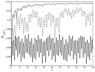
Figure 3: Dynamics of the linear entropy for $\lambda=1/2$ (solid line), $\lambda=1$ (dashed line), and $\lambda=1.5$ (connected dotted line). The parameters $N=144$ and $\sigma=89/144$.

In this paper, we have studied bipartite entanglment of one-particle states, and found a direct connection between the linear entropy, quantifying the bipartite entanglement, and the participation ratio, characterizing state localization. The more localized the state is, the less the entanglement. Pairwise entanglement, bipartite entanglement, and state localization are found closely connected together for one-particle states.

As an application of the general formalism, we have studied quantum entanglement of the ground state in the Harper model and find that the bipartite entanglement exhibits a transition at critical point $\lambda=\lambda_{c}$. The time evolution of entanglement was also investigated, which displays distinct behaviors for different amplitudes of the on-site potential, corresponding to extended, critical, and localized states.

- (1) M.A. Nielsen and I.L. Chuang, Quantum Computation and Quantum Information, Cambridge University Press, 2000.
- (2) C.H. Bennett, G. Brassard, C. Crepeau, R. Jozsa, A. Peres and W.K. Wootters, Phys. Rev. Lett. 70, 1895 (1993).
- (3) C.H. Bennett and S.J. Wiesner, Phys. Rev. Lett. 69, 2881 (1992).
- (4) A.K. Ekert, Phys. Rev. Lett. 67, 661 (1991).
- (5) M. Murao, D. Jonathan, M.B. Plenio, and V. Vedral, Phys. Rev. A, 59, 156 (1999).
- (6) M.A. Nielsen, Ph.D thesis, University of Mexico (1998), e-print quant-ph/0011036.
- (7) M.C. Arnesen, S. Bose, and V. Vedral, Phys. Rev. Lett. 87, 017901 (2001).
- (8) X. Wang, Phys. Rev. A, 64, 012313 (2001).
- (9) K.M. O’Connor and W.K. Wootters, Phys. Rev. A 63, 052302 (2001).
- (10) D. Gunlycke, S. Bose, V.M. Kendon, and V. Vedral, Phys. Rev. A 64, 042302 (2001).
- (11) P. Zanardi, Phys. Rev. A 65, 042101 (2002); P. Zanardi and X. Wang, J. Phys. A: Math. Gen. 35, 7947 (2002).
- (12) T.J. Osborne and M.A. Nielsen, Phys. Rev. A 66, 032110 (2002).
- (13) A. Osterloh, L. Amico, G. Falci and R. Fazio, Nature(London) 416, 608 (2002).
- (14) A. Lakshminarayan and V. Subrahmanyam, Phys. Rev. A 67, 052304 (2003).
- (15) S. Hill and W.K. Wootters, Phys. Rev. Lett. 78, 5022 (1997); W.K. Wootters, ibid. 80, 2245 (1998).
- (16) R. Artuso et al., Int. J. Mod. Phys. B 8, 207 (1994); H. Hiramoto and M. Kohmoto, ibid, 8, 281 (1996).
- (17) W. Dür, G. Vidal, and J.I. Cirac, Phys. Rev. A62, 062314 (2000); W. Dür, Phys. Rev. A63, 020303 (2001).
- (18) C.H. Bennett, H.J. Bernstein, S. Popescu and B. Schumacher, Phys. Rev. A 53,2046 (1996).
- (19) B. Georgeot and D.L. Shepelyansky, Phys. Rev. E 62, 3504 (2000).
- (20) X. Wang, H.B. Li, and B. Hu, unpublished.
- (21) T. Geisel, R. Ketzmerick, and G. Petschel, Phys. Rev. Lett. 66, 1651 (1991).
- (22) D.S. Abrams and S. Lloyd, Phys. Rev. Lett. 79, 2586 (1997); S.B. Bravyi and A.Yu. Kitaev, quant-ph/0003137.