Probabilistic quantum multimeters

Abstract

We propose quantum devices that can realize probabilistically different projective measurements on a qubit. The desired measurement basis is selected by the quantum state of a program register. First we analyze the phase-covariant multimeters for a large class of program states, then the universal multimeters for a special choice of program. In both cases we start with deterministic but erroneous devices and then proceed to devices that never make a mistake but from time to time they give an inconclusive result. These multimeters are optimized (for a given type of a program) with respect to the minimum probability of inconclusive result. This concept is further generalized to the multimeters that minimize the error rate for a given probability of an inconclusive result (or vice versa). Finally, we propose a generalization for qudits.

I Introduction

Programmable quantum multimeters are devices that can realize any desired generalized quantum measurement from a chosen set (either exactly or approximately) DuBu ; FiDuFi . Their main feature is that the particular positive operator valued measure (POVM) is selected by the quantum state of a “program register” (quantum software). In this sense they are analogous to universal quantum processors Nielsen97 ; Vidal00 ; Hillery02 ; Hillery02b . The multimeter itself is represented by a fixed joint POVM on the data and program systems together (see Fig. 1). Each outcome of this POVM is associated with one outcome of the “programmed” POVM on the data alone. From the mathematical point of view the realization of a particular quantum multimeter is equivalent to the optimal discrimination of certain mixed states. A different kind of a quantum multimeter that can be programmed to evaluate the expectation value of any operator has been introduced in Ref. Paz03 . Besides quantum multimeters, other devices whose operation is based on the joint measurement on two different registers have been proposed recently. The universal quantum matching machine that allows to decide which template state is closest to the input feature state was analyzed in Sasaki02 . The problem of comparison of quantum states was studied in BaChJe . The so-called universal quantum detectors have been considered in DAriano03 . All these devices could play an important role in quantum state estimation and quantum information processing.

In this paper, we will describe programmable quantum devices that can accomplish von Neumann measurements on a single qubit. However, it is impossible to perfectly encode arbitrary projective measurement on a qubit into a state in finite-dimensional Hilbert space DuBu . The proof of this theorem is similar to the proof that it is impossible to encode an arbitrary unitary operation (acting on a finite-dimensional Hilbert space) into a state of a finite-dimensional quantum system Nielsen97 . Briefly, one can show that any two program states that perfectly encode two different measurement bases must be mutually orthogonal. Nevertheless, it is still possible to encode POVMs that represent, in a certain sense, the best approximation of the required projective measurements.

A specific way of approximation of projective measurements is a “probabilistic” measurement that allows for some inconclusive results. In this case, instead of a two-component projective measurement one has a three-component POVM and the third outcome corresponds to the inconclusive result. The natural request is to minimize the error rate at the first two outcomes. As a limit case it is possible to get an error-free operation (however, with a nonzero probability of an inconclusive result) – such a multimeter performs the exact projective measurements but with the probability of success lower than one. Such a device is conceptually analogous to the probabilistic programmable quantum gates Nielsen97 ; Vidal00 ; Hillery02 . The other boundary case is an ambiguous multimeter without inconclusive results FiDuFi .

Our present article is organized as follows. In Sec. II we start with the analysis of phase-covariant multimeters that can perform von Neumann measurement on a single qubit in any basis located on the equator of the Bloch sphere. First we discuss deterministic devices (no inconclusive results but errors may appear), then error-free probabilistic devices (no errors but inconclusive results may appear), and finally general multimeters with given fraction of inconclusive results optimized with respect to minimal error-rate. In this section we also introduce and explain in detail all necessary mathematical tools. Further, in Sec. III we study universal multimeters that can accomplish any von Neumann measurement on a single qubit. We confine our investigation to the program consisting of the two basis vectors. Again, we start with deterministic devices, continue with error-free multimeters and finally proceed to apparatuses with a given fraction of inconclusive results. Sec. IV is devoted to probabilistic error-free universal multimeters that can accomplish any projective measurement on a qudit. Sec. V concludes the paper with a short summary.

II Phase-covariant multimeters

In this section we will consider multimeters that should perform von Neumann measurement on a single qubit in any basis $\{|\psi_{+}\rangle,|\psi_{-}\rangle\}$ located on the equator of the Bloch sphere,

$$|\psi_{\pm}(\phi)\rangle=\frac{1}{\sqrt{2}}(|0\rangle\pm e^{i\phi}|1\rangle),$$ (1)

where $\phi\in[0,2\pi]$ is arbitrary. To simplify notation, we shall not usually display the dependence of the basis states on $\phi$ explicitly in what follows. Generally, the design of the optimal multimeter should involve the optimization of both the dependence of the program on the measurement basis and the fixed joint measurement on the program and data states. However, this is a very hard problem that we will not attempt to solve in its generality. Instead, we will design an optimal multimeter for a particular simple and natural choice of the program. Namely, similarly as in FiDuFi , we assume that the program of the multimeter $|\Psi\rangle_{\mathrm{p}}$ which determines the measurement basis consists of $N$ copies of the basis state $|\psi_{+}\rangle$, $|\Psi\rangle_{\mathrm{p}}=|\psi_{+}\rangle^{\otimes N}$. Since we have restricted ourselves to the bases (1), the state $|\psi_{-}\rangle$ can be obtained form $|\psi_{+}\rangle$ via unitary transformation,

$$|\psi_{-}\rangle=\sigma_{z}|\psi_{+}\rangle,$$ (2)

where $\sigma_{z}$ denotes the Pauli matrix. This implies that all the programs of the form $|\psi_{+}\rangle^{\otimes j}|\psi_{-}\rangle^{\otimes N-j}$ are equivalent to the program $|\psi_{+}\rangle^{N}$ because these programs are related via a fixed unitary $U=\openone^{\otimes j}\otimes\sigma_{z}^{\otimes N-j}$. First, we shall derive the optimal deterministic multimeter, which always yields an outcome, but errors may occur. Then, we shall consider a probabilistic multimeter that conditionally realizes exactly the von-Neumann measurement in basis (1), but at the expense of some fraction of inconclusive results. Finally, we will show that the deterministic and unambiguous multimeters are just two extremal cases from a whole class of optimal multimeters that are designed such that the probability of correct measurement on basis states is maximized for a fixed fraction of inconclusive results.

Figure 1: Schematic drawing of a quantum multimeter. The effective measurement performed on the data state $\rho$ is selected by the quantum state of the program register $|\Psi\rangle_{\mathrm{p}}$. The multimeter itself carries out a fixed joint generalized measurement on data and program states which is described by a POVM $\{\Pi_{j}\}$.

II.1 Deterministic multimeter

The multimeter is a device that performs a joint generalized measurement described by the POVM $\{\Pi_{j}\}$ on the data state and the program state, see Fig. 1. This fixed joint measurement on the data and program can be also interpreted as an effective measurement on the data register, which is described by the POVM ${\pi_{j}}$ and depends of the program via

$$\pi_{j}=\mathrm{Tr}_{\mathrm{p}}[(\openone_{\mathrm{d}}\otimes|\Psi\rangle_{\mathrm{p}}\langle\Psi|)\,\Pi_{j}],$$ (3)

where the subscripts $\mathrm{d}$ and $\mathrm{p}$ denote the data and program states, respectively. The deterministic single-qubit multimeter is fully characterized by a two-component POVM $\{\Pi_{+},\Pi_{-}\}$. The readout of $\Pi_{+}$ is interpreted as the finding of the data state in basis state $|\psi_{+}\rangle$ while $\Pi_{-}$ is associated with the detection of $|\psi_{-}\rangle$. Ideally,

$$\pi_{\pm}=|\psi_{\pm}\rangle\langle\psi_{\pm}|$$ (4)

should hold, but this cannot be achieved for all $\phi$ with a finite-dimensional program.

The performance of the multimeter is quantified by the probability $P_{S}$ that the measurement yields correct outcome when the data register is prepared in the basis state $|\psi_{+}\rangle$ or $|\psi_{-}\rangle$ with probability $1/2$ each. For each particular phase $\phi$ we thus have

$$P_{S}(\phi) = \frac{1}{2}\mathrm{Tr}[\Pi_{+}\psi_{+}(\phi)\otimes\psi_{+}^{\otimes N}(\phi)]+$$ (5)

$$\frac{1}{2}\mathrm{Tr}[\Pi_{-}\psi_{-}(\phi)\otimes\psi_{+}^{\otimes N}(\phi)],$$

where $\psi_{\pm}=|\psi_{\pm}\rangle\langle\psi_{\pm}|$. Assuming homogeneous a-priori distribution of the angle $\phi$ we define the average success rate as

$$P_{S}=\int_{0}^{2\pi}P_{S}(\phi)\frac{d\phi}{2\pi}.$$ (6)

We define the optimal deterministic multimeter as the multimeter that maximizes $P_{S}$ for the program $|\psi_{+}\rangle^{\otimes N}$. The choice of $P_{S}$ as the figure of merit is strongly supported by the observation that $P_{S}$ can be interpreted as the average fidelity of the multimeter. Consider the effective POVM on the data qubit $\{\pi_{+}(\phi),\pi_{-}(\phi)\}$ for some particular phase $\phi$. It is natural to define the fidelity of this POVM with respect to the projective measurement in the basis $|\psi_{\pm}(\phi)\rangle$ as follows,

$$F(\phi) = \frac{1}{2}\langle\psi_{+}(\phi)|\pi_{+}(\phi)|\psi_{+}(\phi)\rangle+$$

$$\frac{1}{2}\langle\psi_{-}(\phi)|\pi_{-}(\phi)|\psi_{-}(\phi)\rangle.$$

It is easy to see that the average fidelity $F=\frac{1}{2\pi}\int_{0}^{2\pi}F(\phi)d\phi$ coincides with the average success rate (6). Clearly, $F\leq 1$ and $F=1$ if and only if (4) holds for all $\phi$ (maybe except of a set of measure zero).

To simplify the notation we introduce the symbol $C_{N,k}$ for the binomial coefficient,

$$C_{N,k}={N\choose k}.$$ (7)

On inserting the formula for $P_{S}(\phi)$ into Eq. (6) and carrying out the integration over $\phi$ we find that

$$P_{S}=\frac{1}{2}(\mathrm{Tr}[\Pi_{+}R_{+}]+\mathrm{Tr}[\Pi_{-}R_{-}]),$$ (8)

where the two positive semidefinite operators $R_{\pm}$ read

$$R_{+} = \frac{1}{2^{N+1}}\sum_{k=1}^{N}C_{N+1,k}|\varphi_{N,k}^{+}\rangle\langle\varphi_{N,k}^{+}|+\frac{1}{2^{N+1}}X$$

$$R_{-} = \frac{1}{2^{N+1}}\sum_{k=1}^{N}C_{N+1,k}|\varphi_{N,k}^{-}\rangle\langle\varphi_{N,k}^{-}|+\frac{1}{2^{N+1}}X.$$

Here

$$|\varphi_{N,k}^{\pm}\rangle=\sqrt{1-B_{N,k}}\,|0\rangle_{\mathrm{d}}|N,k\rangle_{\mathrm{p}}\pm\sqrt{B_{N,k}}\,|1\rangle_{\mathrm{d}}|N,k-1\rangle_{\mathrm{p}},$$ (9)

with $B_{N,k}=k/(N+1)$. The operator $X$ that is common to $R_{+}$ and $R_{-}$ is given by

$$X=|0\rangle_{\mathrm{d}}\langle 0|\otimes|N,0\rangle_{\mathrm{p}}\langle N,0|+|1\rangle_{\mathrm{d}}\langle 1|\otimes|N,N\rangle_{\mathrm{p}}\langle N,N|,$$ (10)

and $|N,k\rangle$ denotes a normalized totally symmetric state of $N$ qubits with $k$ qubits in state $|1\rangle$ and $N-k$ qubits in state $|0\rangle$.

It follows from Eq. (8) that the optimal deterministic multimeter is the one that optimally discriminates between two mixed states $R_{+}$ and $R_{-}$. This problem has been analyzed by Helstrom helst who showed that the maximal achievable success rate is

$$P_{S,\mathrm{max}}=\frac{1}{2}+\frac{1}{4}\mathrm{Tr}|R_{+}-R_{-}|$$ (11)

and the optimal POVM is given by projectors onto the subspaces spanned by the eigenstates of $\Delta R=R_{+}-R_{-}$ with positive and negative eigenvalues, respectively. If some of the eigenvalues of $\Delta R$ are zero, then the projectors can be freely added either to $\Pi_{+}$ or $\Pi_{-}$.

In the basis $|0\rangle_{\mathrm{d}}|N,k\rangle_{\mathrm{p}}$, $|1\rangle_{\mathrm{d}}|N,k\rangle_{\mathrm{p}}$, the matrix $\Delta R$ is block diagonal and its eigenvalues and eigenstates can easily be determined. Since $\mathrm{Tr}|\Delta R|$ is equal to the sum of absolute values of the eigenvalues of $\Delta R$, we find after simple algebra that

$$P_{S,\mathrm{max}}=\frac{1}{2}+\frac{1}{2^{N+1}}\sum_{k=1}^{N}\sqrt{{N\choose k}{N\choose k-1}}.$$ (12)

Interestingly enough, $P_{S,\mathrm{max}}$ is equal to the optimal fidelity of estimation of $|\psi_{+}(\phi)\rangle$ from $N$ copies of $|\psi_{+}(\phi)\rangle$ DeBuEk . So one possible implementation of the optimal deterministic phase-covariant multimeter with program $|\psi_{+}(\phi)\rangle^{\otimes N}$ would be to first carry out the optimal estimation of $|\psi_{+}(\phi)\rangle$ and then measure the data qubit in the basis spanned by the estimated state and its orthogonal counterpart. Instead, one could also perform a joint generalized measurement on data and program. The two POVM elements are given by

$$\Pi_{\pm}=\sum_{k=1}^{N}|\Pi_{N,k}^{\pm}\rangle\langle\Pi_{N,k}^{\pm}|+\frac{1}{2}X,$$ (13)

where

$$|\Pi_{N,k}^{\pm}\rangle=\frac{1}{\sqrt{2}}(|0\rangle_{\mathrm{d}}|N,k\rangle_{\mathrm{p}}\pm|1\rangle_{\mathrm{d}}|N,k-1\rangle_{\mathrm{p}}).$$ (14)

The effective POVM on the data register (3) can be expressed as

$$\pi_{\pm}=P_{S,\mathrm{max}}|\psi_{\pm}\rangle\langle\psi_{\pm}|+(1-P_{S,\mathrm{max}})|\psi_{\mp}\rangle\langle\psi_{\mp}|.$$ (15)

In the limit of infinitely large program register, $N\rightarrow\infty$, the POVM (15) approaches the ideal projective measurement (4).

II.2 Error-free probabilistic multimeter

The multimeter designed in the preceding section is only approximate, because the effective POVM (15) on the data register differs from the projective measurement in the basis $|\psi_{+}\rangle$, $|\psi_{-}\rangle$. Here, we construct a multimeter that realizes an exact von Neumann measurement in the basis (1) with some probability $P_{S}$. This is achieved at the expense of the inconclusive results which occur with the probability $P_{I}=1-P_{S}$ and are associated with the POVM element $\Pi_{?}$. Such a probabilistic multimeter must unambiguously discriminate between two mixed states $R_{+}$ and $R_{-}$. The unambiguous discrimination of mixed quantum states RuSpTu ; RaLuEn (and, more generally, discrimination of mixed states with inconclusive results FiJe ; El ) has attracted a considerable attention recently.

As formally stated in Ref. RuSpTu , we have to find a three-component POVM $\Pi_{+},\Pi_{-},\Pi_{?}$ that maximizes the success rate (8) under the constraints

$$\mathrm{Tr}[\Pi_{+}R_{-}]=\mathrm{Tr}[\Pi_{-}R_{+}] = 0,$$

$$\Pi_{+}+\Pi_{-}+\Pi_{?} = \openone,$$

$$\Pi_{+}\geq 0,\quad\Pi_{-}\geq 0,\quad\Pi_{?} \geq 0,$$ (16)

which is an instance of the so-called semidefinite program. The first constraint guarantees that the multimeter will never respond with a wrong outcome, i.e. $\Pi_{-}$ ($\Pi_{+}$) cannot be detected when the data register is in the basis state $|\psi_{+}\rangle$ ($|\psi_{-}\rangle$). The second and third constraints express the completeness of the POVM and the positive semidefiniteness of the POVM elements.

Here we shall give a simple intuitive construction of the optimal POVM and we shall analyze the dependence of $P_{I}$ on $N$. The optimality of the POVM will be formally proved in the next subsection using the techniques introduced in Ref. FiJe .

Due to the particular structure of the operators $R_{+}$ and $R_{-}$ the problem of unambiguous discrimination of $R_{+}$ and $R_{-}$ splits into $N$ independent problems of unambiguous discrimination of two pure states $|\varphi_{N,k}^{+}\rangle$ and $|\varphi_{N,k}^{-}\rangle$. The unambiguous discrimination of two pure non-orthogonal states with equal a-priori probabilities has been studied by Ivanovic ivanovic , Dieks dieks , and Peres peres (IDP). The minimal probability of inconclusive results is equal to the absolute value of the scalar product of the two states. Taking this into account, we can immediately write down $P_{I}$ for the optimal unambiguous phase-covariant multimeter,

$$P_{I}=\frac{1}{2^{N+1}}\sum_{k=1}^{N}\,C_{N+1,k}\left|\langle\varphi_{N,k}^{+}|\varphi_{N,k}^{-}\rangle\right|+\frac{1}{2^{N}}.$$ (17)

The contribution $2^{-N}$ to $P_{I}$ stems from the term $X$ that is common to both operators $R_{\pm}$. On inserting the expression (9) into Eq. (17) we obtain

$$P_{I}=\frac{1}{2^{N+1}}\sum_{k=1}^{N}\,\left|C_{N,k}-C_{N,k-1}\right|+\frac{1}{2^{N}}.$$ (18)

We must distinguish the cases of odd and even $N$. Let us assume that $N$ is even ($N=2n$). We divide the sum in Eq. (18) into two parts $k\leq N/2$ and $k>N/2$ and we find

$$\sum_{k=1}^{N}\left|C_{N,k}-C_{N,k-1}\right|=2{N\choose N/2}-2.$$ (19)

On inserting the sum back into Eq. (18) we obtain

$$P_{I}(2n)=\frac{1}{2^{2n}}{2n\choose n}.$$ (20)

The calculation for odd $N=2n-1$ proceeds along similar lines and one obtains

$$P_{I}(2n-1)=\frac{1}{2^{2n-1}}{2n-1\choose n-1}.$$ (21)

It holds that $P_{I}(2n-1)=P_{I}(2n)$ hence the error-free probabilistic phase-covariant multimeter with $2n-1$ qubit program is exactly as efficient as the multimeter with $2n$-qubit program. It is worth noting here that a similar behavior has been observed in the context of optimal $1\rightarrow N$ phase covariant cloning of qubits DArMa where it was found that the global fidelities of clones produced by the $1\rightarrow 2n$ and $1\rightarrow 2n+1$ cloning machines are equal. The asymptotic behavior of the probability of inconclusive results (20) and (21) can be extracted with the help of the Stirling’s formula $N!\approx\sqrt{2\pi N}\,N^{N}e^{-N}$. On inserting this approximation into (20) we get $P_{I}(N)\approx 2/\sqrt{2\pi N}.$

The POVM elements that describe the optimal error-free multimeter can be easily written down as the properly weighted convex sum of the POVM elements that describe the optimal unambiguous discrimination of the states $|\varphi_{N,k}^{+}\rangle$ and $|\varphi_{N,k}^{-}\rangle$,

$$\Pi_{+}=\sum_{k=1}^{N}D_{N,k}^{-1}|\varphi_{\perp,N,k}^{-}\rangle\langle\varphi_{\perp,N,k}^{-}|,$$

$$\Pi_{-}=\sum_{k=1}^{N}D_{N,k}^{-1}|\varphi_{\perp,N,k}^{+}\rangle\langle\varphi_{\perp,N,k}^{+}|,$$ (22)

and $\Pi_{?}=\openone-\Pi_{+}-\Pi_{-}$. Here $|\varphi_{\perp,N,k}^{\pm}\rangle$ denote states orthogonal to $|\varphi_{N,k}^{\pm}\rangle$, respectively,

$$|\varphi_{\perp,N,k}^{\pm}\rangle=\sqrt{B_{N,k}}\,|0\rangle_{\mathrm{d}}|N,k\rangle_{\mathrm{p}}\mp\sqrt{1-B_{N,k}}\,|1\rangle_{\mathrm{d}}|N,k-1\rangle_{\mathrm{p}},$$ (23)

and

$$D_{N,k}=\frac{2}{N+1}\max(k,N+1-k).$$ (24)

The effective three-component POVM on the data register associated with POVM (22) reads

$$\pi_{\pm}=(1-P_{I})|\psi_{\pm}\rangle\langle\psi_{\pm}|,\qquad\pi_{?}=P_{I}\openone.$$ (25)

Note, that when performing a generalized measurement described by the POVM (25) the statistics of the sub-ensemble of conclusive results would exactly agree with the statistics obtained by von Neumann projective measurement in basis $|\psi_{\pm}\rangle$, so the multimeter indeed exactly probabilistically performs the required measurement on the data qubit.

II.3 Multimeter with a fixed fraction of inconclusive results

The deterministic multimeters and the error-free probabilistic multimeters discussed in the preceding subsections can be considered as special limiting cases of a more general class of optimal multimeters that yield an inconclusive result with probability $P_{I}=\mathrm{Tr}[\Pi_{?}(R_{+}+R_{-})/2]$ and give the correct measurement outcome with probability $P_{S}\leq 1-P_{I}$ when the data register is prepared in the basis state $|\psi_{+}(\phi)\rangle$ or $|\psi_{-}(\phi)\rangle$ with equal a-priori probability. It is convenient to introduce the relative success rate

$$P_{RS}=\frac{P_{S}}{1-P_{I}}$$ (26)

which gives the fraction of correct outcomes in the sub-ensemble of conclusive results. Note that $P_{RS}$ can be also interpreted as the average fidelity of the probabilistic multimeter. The optimal multimeter should achieve the maximal possible $P_{S}$ (hence also $P_{RS}$) for a given fixed probability of inconclusive results $P_{I}$. This class of multimeters is described by three-component POVM similarly as the unambiguous (error-free) multimeter. Such multimeters in fact perform the optimal discrimination of mixed quantum states $R_{+}$ and $R_{-}$ with a fixed fraction of inconclusive results. This general quantum-state discrimination scenario has been recently analyzed in detail in Refs. FiJe ; El , where it was shown that the optimal POVM must satisfy the following set of extremal equations:

$$\left(\lambda-\frac{1}{2}R_{\pm}\right)\Pi_{\pm}=0,\qquad\left(\lambda-aR_{?}\right)\Pi_{?}=0,$$ (27)

and

$$\lambda-\frac{1}{2}R_{\pm}\geq 0,\qquad\lambda-aR_{?}\geq 0.$$ (28)

Here $R_{?}=(R_{+}+R_{-})/2$ and $\lambda$ and $a$ are Lagrange multipliers that account for the constraints $\Pi_{+}+\Pi_{-}+\Pi_{?}=\openone$ and

$$\mathrm{Tr}[\Pi_{?}R_{?}]=P_{I}.$$ (29)

It follows from the structure of the extremal Eqs. (27) and (28) that the problem of optimal discrimination of two mixed states $R_{\pm}$ with a fraction of inconclusive results $P_{I}$ is formally equivalent to the maximization of success rate of the deterministic discrimination of three mixed states $R_{+}$, $R_{-}$, and $R_{?}$ with a-priori probabilities $p_{\pm}=1/[2(a+1)]$ and $p_{?}=a/(a+1)$. Of course, this equivalence straightforwardly extends to discrimination of $n$ mixed states.

In the present case, the key simplification stems from the observation that the operators $R_{\pm}$ have a common block diagonal form, which was already explored in construction of the optimal error-free phase-covariant multimeter. Formally, we can write

$$R_{\pm}=\frac{1}{2^{N+1}}\bigoplus_{k=0}^{N+1}R_{\pm,k},$$ (30)

where

$$R_{\pm,k} = C_{N+1,k}|\varphi_{N,k}^{\pm}\rangle\langle\varphi_{N,k}^{\pm}|,\qquad k=1,\ldots,N,$$

$$R_{\pm,0} = |0\rangle_{\mathrm{d}}\langle 0|\otimes|N,0\rangle_{\mathrm{p}}\langle N,0|,$$

$$R_{\pm,N+1} = |1\rangle_{\mathrm{d}}\langle 1|\otimes|N,N\rangle_{\mathrm{p}}\langle N,N|.$$

Accordingly, the total Hilbert space of the data and the program states $\mathcal{H}=\mathcal{H}_{\mathrm{d}}\otimes\mathcal{H}_{\mathrm{p}}$ can be decomposed into a direct sum of $\mathcal{H}_{k}$, $\mathcal{H}=\oplus_{k=0}^{N+1}\mathcal{H}_{k}$. The Hilbert spaces $\mathcal{H}_{k}$ are either two-dimensional (spanned by $|0\rangle_{\mathrm{d}}|N,k\rangle_{\mathrm{p}}$ and $|1\rangle_{\mathrm{d}}|N,k-1\rangle_{\mathrm{p}}$) or one-dimensional (spanned by $|0\rangle_{\mathrm{d}}|N,0\rangle_{\mathrm{p}}$ or $|1\rangle_{\mathrm{d}}|N,N\rangle_{\mathrm{p}}$). The optimal $\Pi_{+}$, $\Pi_{-}$, $\Pi_{?}$ and $\lambda$ also have a block-diagonal structure

$$\Pi_{\pm}=\bigoplus_{k=0}^{N+1}\Pi_{\pm,k},\qquad\Pi_{?}=\bigoplus_{k=0}^{N+1}\Pi_{?,k},\qquad\lambda=\bigoplus_{k=0}^{N+1}\lambda_{k}.$$ (31)

The extremal equations (27) and (28) split into $N+2$ equations

$$\left(\lambda_{k}-\frac{1}{2}R_{\pm,k}\right)\Pi_{\pm,k}=0,\qquad\left(\lambda_{k}-aR_{?,k}\right)\Pi_{?,k}=0,$$ (32)

$$\lambda_{k}-\frac{1}{2}R_{\pm,k}\geq 0,\qquad\lambda_{k}-aR_{?,k}\geq 0.$$ (33)

We thus have to determine the optimal POVM on each subspace $\mathcal{H}_{k}$ and then merge the solutions according to (31). Due to the structure of the operators $R_{\pm}$, the task reduces to the discrimination of two pure non-orthogonal states $|\varphi_{N,k}^{\pm}\rangle$ with inconclusive results, which was discussed in detail by Chefles and Barnett ChBa and also by Zhang et al. Zhang99 .

Let us first consider the non-degenerate case $k=1,\ldots,N$. We have to distinguish the cases $C_{N,k}\geq C_{N,k-1}$ (i.e. $k\leq[N/2]$) and $C_{N,k}<C_{N,k-1}$ ($k>[N/2]$). We will explicitly present the results for $k\leq[N/2]$. The formulas for $k>[N/2]$ are similar and can be obtained by simple exchanges $C_{N,k}\leftrightarrow C_{N,k-1}$ and $|0\rangle_{\mathrm{d}}|N,k\rangle_{\mathrm{p}}\leftrightarrow|1\rangle_{\mathrm{d}}|N,k-1\rangle_{\mathrm{p}}$. The optimal POVM on each subspace $\mathcal{H}_{k}$ can be written as follows

$$\Pi_{+,k} = \frac{1}{2\sin^{2}\Phi_{k}}|\Phi_{N,k}^{+}\rangle\langle\Phi_{N,k}^{+}|,$$

$$\Pi_{-,k} = \frac{1}{2\sin^{2}\Phi_{k}}|\Phi_{N,k}^{-}\rangle\langle\Phi_{N,k}^{-}|,$$

$$\Pi_{?,k} = (1-\tan^{-2}\Phi_{k})|0\rangle_{\mathrm{d}}\langle 0|\otimes|N,k\rangle_{\mathrm{p}}\langle N,k|,$$ (34)

where

$$|\Phi_{N,k}^{+}\rangle=\cos\Phi_{k}|0\rangle_{\mathrm{d}}|N,k\rangle_{\mathrm{p}}\pm\sin\Phi_{k}|1\rangle_{\mathrm{d}}|N,k-1\rangle_{\mathrm{p}}.$$ (35)

The angle $\Phi_{k}$ is a function of the Lagrange multiplier $a$. This dependence can be determined by substituting the explicit form of the optimal POVM (34) into the extremal Eqs. (32) and solving the resulting system of linear equations for $\lambda_{k}$ and $a$. After a bit tedious but otherwise straightforward algebra we obtain

$$\tan\Phi_{k}=\left\{\begin{array}[]{lll}1,&&a<a_{\mathrm{th,k}},\\ \sqrt{\frac{C_{N,k}}{C_{N,k-1}}}(2a-1),&&a\geq a_{\mathrm{th},k},\end{array}\right.$$ (36)

where $a_{\mathrm{th},k}=\frac{1}{2}\left(1+\sqrt{C_{N,k-1}/C_{N,k}}\right)$. The probability of inconclusive results $P_{I,k}$ and the probability of correct guess $P_{S,k}$ when discriminating the states $|\varphi_{N,k}^{\pm}\rangle$ with the POVM (34) are given by

$$P_{I,k} = \frac{C_{N,k}}{C_{N+1,k}}\left(1-\frac{1}{\tan^{2}\Phi_{k}}\right),$$

$$P_{S,k} = \frac{\cos^{2}(\Phi_{k}-\Theta_{k})}{2\sin^{2}\Phi_{k}},$$ (37)

where $\Theta_{k}=\arctan(\sqrt{C_{N,k-1}/C_{N,k}})$.

The cases $k=0$ and $k=N+1$ require special treatment because the two states to be discriminated are actually identical. Let us consider the case $k=0$. If $a\neq 1/2$ then the optimal POVM can be formally determined from Eqs. (34) and (36) where the limit $C_{N,k-1}\rightarrow 0$ must be considered. One finds that $\Pi_{?,0}=0$ for $a<1/2$ while $\Pi_{+,0}=\Pi_{-,0}=0$ and $\Pi_{?,0}=\openone_{0}$ for $a>1/2$. A sharp transition occurs at $a=1/2$ where the optimal POVM changes from projective measurement to a single-component POVM with all measurement outcomes being interpreted as inconclusive results. The transition at $a=1/2$ can be described by a single parameter $\eta\in[0,1]$ and we can write

$$\Pi_{\pm,0} = \frac{1}{2}(1-\eta)|0\rangle_{\mathrm{d}}\langle 0|\otimes|N,0\rangle_{\mathrm{p}}\langle N,0|,$$

$$\Pi_{?,0} = \eta|0\rangle_{\mathrm{d}}\langle 0|\otimes|N,0\rangle_{\mathrm{p}}\langle N,0|.$$

Consequently, we have $P_{S,0}=1/2$, $P_{I,0}=0$ for $a<1/2$; $P_{S,0}=0$, $P_{I,0}=1$ for $a>1/2$ and a smooth transition $P_{S,0}=(1-\eta)/2$, $P_{I,0}=\eta$ at $a=1/2.$

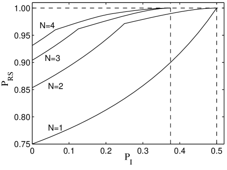
Figure 2: Dependence of the relative success rate $P_{RS}$ of the optimal phase-covariant multimeter with program $|\psi_{+}\rangle^{\otimes N}$ on the fraction of inconclusive results $P_{I}$.

The class of the optimal probabilistic phase covariant multimeters is thus parameterized by two numbers $a\in[0,1]$ and $\eta\in[0,1]$. If we combine all the above derived results we can express the dependence of $P_{S}$ on $a$ and $\eta$ as follows,

$$P_{S}=\frac{1}{2^{N+1}}\sum_{k=1}^{N}C_{N+1,k}P_{S,k}+\frac{1}{2^{N+1}}(P_{S,0}+P_{S,N+1}),$$ (38)

and a similar formula holds also for $P_{I}$. Rather than plotting the dependence of $P_{S}$ and $P_{I}$ on $a$ and $\eta$, we directly show in Fig. 2 the dependence of the relative success rate $P_{RS}=P_{S}/(1-P_{I})$ (i.e., the fidelity of the probabilistic multimeter) on the fraction of inconclusive results $P_{I}$. We can see that $P_{RS}$ monotonically grows with $P_{I}$ and the point of unambiguous probabilistic operation is indicated by $P_{RS}=1$, when $P_{I}$ has the value given by Eqs. (20) and (21). Taking into account the symmetry of the POVM (34) with respect to the exchanges $k\rightarrow N-k+1$ and $|0\rangle_{\mathrm{d}}\rightarrow|1\rangle_{\mathrm{d}}$ it is easy to show that the effective POVM on the data qubit corresponding to the optimal POVM (34) is given by

$$\pi_{\pm} = (1-P_{I})\left[P_{RS}|\psi_{\pm}\rangle\langle\psi_{\pm}|+(1-P_{RS})|\psi_{\mp}\rangle\langle\psi_{\mp}|\right],$$

$$\pi_{?} = P_{I}\openone.$$

The POVM has this structure for all possible program states (i.e., all measurement bases) hence the multimeter is indeed universal and covariant. Since the POVM element $\pi_{?}$ is proportional to the identity operator the detection of an inconclusive result does not provide any information on the data state.

III Universal multimeters for qubits

In this section we will relax the confinement on the bases consisting of vectors from the equator of the Bloch sphere and will study universal multimeters designed for measurement in any basis represented by two orthogonal states $|\psi_{+}\rangle=\cos\frac{\vartheta}{2}|0\rangle+e^{i\phi}\sin\frac{\vartheta}{2}|1\rangle$ and $|\psi_{-}\rangle=\sin\frac{\vartheta}{2}|0\rangle-e^{i\phi}\cos\frac{\vartheta}{2}|1\rangle$. We want this measurement basis be controlled by the quantum state of a program register, $|\Psi(\psi)\rangle_{\mathrm{p}}$. The program will be assumed in the simplest symmetric form defining the measurement basis: $|\Psi(\psi)\rangle_{\mathrm{p}}=|\psi_{+}\rangle|\psi_{-}\rangle$.

III.1 Deterministic multimeter

First, let us assume the multimeter that always “works” but that allows for some erroneous results. Such a deterministic multimeter was analyzed in Ref. FiDuFi . The optimal (in the sense of the minimum error rate) two-component POVM can be obtained in the similar way as in Sec. II.1. In fact the task is equivalent to the discrimination of two mixed states

$$R_{+} = \int_{\psi}d\psi\,|\Psi_{+}\rangle\langle\Psi_{+}|,$$

$$R_{-} = \int_{\psi}d\psi\,|\Psi_{-}\rangle\langle\Psi_{-}|,$$ (39)

where averaging goes over all bases in the qubit space, i.e., over the whole surface of the Bloch sphere, $\int_{\psi}d\psi=\frac{1}{4\pi}\int_{0}^{\pi}\int_{0}^{2\pi}\,\sin\vartheta\,d\vartheta\,d\phi$, and

$$|\Psi_{+}\rangle = |\psi_{+}\rangle_{\mathrm{d}}\otimes|\psi_{+}\rangle|\psi_{-}\rangle_{\mathrm{p}},$$

$$|\Psi_{-}\rangle = |\psi_{-}\rangle_{\mathrm{d}}\otimes|\psi_{+}\rangle|\psi_{-}\rangle_{\mathrm{p}}.$$

After some algebra we obtain

$$R_{\pm}=\frac{1}{12}\Pi_{\mathrm{sym}}+\frac{1}{3}|A_{\pm}\rangle\langle A_{\pm}|+\frac{1}{3}|B_{\pm}\rangle\langle B_{\pm}|,$$ (40)

where $\Pi_{\mathrm{sym}}$ is the projector on the symmetric subspace of three qubits and the eigenvectors $|A_{\pm}\rangle$ and $|B_{\pm}\rangle$ can be expressed in the computational basis as follows

$$|A_{+}\rangle = \frac{1}{\sqrt{6}}(|0\rangle_{\mathrm{d}}|11\rangle_{\mathrm{p}}+|1\rangle_{\mathrm{d}}|01\rangle_{\mathrm{p}}-2|1\rangle_{\mathrm{d}}|10\rangle_{\mathrm{p}}),$$

$$|B_{+}\rangle = \frac{1}{\sqrt{6}}(-2|0\rangle_{\mathrm{d}}|01\rangle_{\mathrm{p}}+|0\rangle_{\mathrm{d}}|10\rangle_{\mathrm{p}}+|1\rangle_{\mathrm{d}}|00\rangle_{\mathrm{p}});$$

$$|A_{-}\rangle = \frac{1}{\sqrt{6}}(-|0\rangle_{\mathrm{d}}|11\rangle_{\mathrm{p}}+2|1\rangle_{\mathrm{d}}|01\rangle_{\mathrm{p}}-|1\rangle_{\mathrm{d}}|10\rangle_{\mathrm{p}}),$$

$$|B_{-}\rangle = \frac{1}{\sqrt{6}}(-|0\rangle_{\mathrm{d}}|01\rangle_{\mathrm{p}}+2|0\rangle_{\mathrm{d}}|10\rangle_{\mathrm{p}}-|1\rangle_{\mathrm{d}}|00\rangle_{\mathrm{p}}).$$

Notice the important orthogonality properties

$$\langle A_{+}|B_{+}\rangle=\langle A_{-}|B_{-}\rangle = \langle A_{+}|B_{-}\rangle=\langle A_{-}|B_{+}\rangle=0,$$

$$\langle A_{+}|A_{-}\rangle = \langle B_{+}|B_{-}\rangle=\frac{1}{2}.$$

Moreover, the states (LABEL:AB) are also orthogonal to any state from the symmetric subspace of three qubits.

As shown in Ref. FiDuFi , the optimal POVM for the deterministic discrimination of the mixed states (40) has the following form:

$$\Pi_{+} = \frac{1}{2}\Pi_{\mathrm{sym}}+|\phi_{1}\rangle\langle\phi_{1}|+|\phi_{2}\rangle\langle\phi_{2}|,$$

$$\Pi_{-} = \openone-\Pi_{+},$$ (42)

where $\openone$ is an identity operator on Hilbert space of three qubits, and

$$|\phi_{1}\rangle = \frac{1}{2\sqrt{3}}[(\sqrt{3}+1)|0\rangle_{\rm d}|01\rangle_{\rm p}-(\sqrt{3}-1)|0\rangle_{\rm d}|10\rangle_{\rm p}$$

$$-2\,|1\rangle_{\rm d}|00\rangle_{\rm p}],$$

$$|\phi_{2}\rangle = \frac{1}{2\sqrt{3}}[(\sqrt{3}+1)|1\rangle_{\rm d}|10\rangle_{\rm p}-(\sqrt{3}-1)|1\rangle_{\rm d}|01\rangle_{\rm p}$$ (43)

$$-2\,|0\rangle_{\rm d}|11\rangle_{\rm p}].$$

Corresponding maximal success rate (probability of a correct result) is

$$P_{S,\mathrm{max}}=\frac{1}{2}\left(1+\frac{1}{\sqrt{3}}\right).$$

For any program $|\psi_{+}\rangle|\psi_{-}\rangle_{\mathrm{p}}$ the effective POVM on the data qubit is given by Eq. (15) hence the multimeter is universal and works equally well for all bases.

III.2 Probabilistic error-free multimeter

Let us now deal with the situation when we want to avoid any errors. So we are looking for such a three-component POVM ($\Pi_{+},\Pi_{-},\Pi_{?}$) acting on data and program together that gives three results according to the following prescription:

Similarly as in Sec. II, the mean probability of an inconclusive result is defined by $P_{I}=\frac{1}{2}\mathrm{Tr}[\Pi_{?}(R_{+}+R_{-})]$ and $\Pi_{?}$ is the POVM component corresponding to an inconclusive result.

Our aim is to find POVM that never wrongly identifies states $|\Psi_{+}\rangle$ and $|\Psi_{-}\rangle$ for any choice of basis $|\psi_{\pm}\rangle$ and that, at the same time, minimizes the probability of inconclusive result. This problem is formally equivalent to the determination of the optimal POVM for unambiguous discrimination of two mixed states $R_{+}$ and $R_{-}$. It means that, similarly as in Sec. II.2, we are looking for operators $\Pi_{+},\Pi_{-},\Pi_{?}$ minimizing $P_{I}$ under the constraints (16), where the relevant $R_{\pm}$ are defined by Eq. (39).

The optimal POVM for the unambiguous discrimination of these two mixed states consists of the multiples of projectors onto the kernels of $R_{+}$ and $R_{-}$ (and of the supplement to unity). The outcome $\Pi_{+}$ can be invoked only by $R_{+}$, the outcome $\Pi_{-}$ only by $R_{-}$. We get

$$\Pi_{+} = \frac{2}{3}\left[|\chi_{1}\rangle\langle\chi_{1}|+|\chi_{2}\rangle\langle\chi_{2}|\right],$$

$$\Pi_{-} = \frac{2}{3}\left[|\kappa_{1}\rangle\langle\kappa_{1}|+|\kappa_{2}\rangle\langle\kappa_{2}|\right],$$

$$\Pi_{?} = \openone-\Pi_{+}-\Pi_{-},$$ (44)

where

$$|\chi_{1}\rangle = \frac{1}{\sqrt{2}}(|0\rangle_{\mathrm{d}}|01\rangle_{\mathrm{p}}-|1\rangle_{\mathrm{d}}|00\rangle_{\mathrm{p}}),$$

$$|\chi_{2}\rangle = \frac{1}{\sqrt{2}}(|0\rangle_{\mathrm{d}}|11\rangle_{\mathrm{p}}-|1\rangle_{\mathrm{d}}|10\rangle_{\mathrm{p}}),$$

$$|\kappa_{1}\rangle = \frac{1}{\sqrt{2}}(|0\rangle_{\mathrm{d}}|10\rangle_{\mathrm{p}}-|1\rangle_{\mathrm{d}}|00\rangle_{\mathrm{p}}),$$

$$|\kappa_{2}\rangle = \frac{1}{\sqrt{2}}(|0\rangle_{\mathrm{d}}|11\rangle_{\mathrm{p}}-|1\rangle_{\mathrm{d}}|01\rangle_{\mathrm{p}}).$$

This POVM leads to the lowest probability of inconclusive result that equals $2/3$.

The proof of optimality follows the same lines as in Sec. II.2. Due to the particular structure of operators $R_{+}$ and $R_{-}$ the problem of their unambiguous discrimination splits into independent problems of the unambiguous discrimination of two pure states. This can be most easily seen from the spectral decomposition of $R_{+}$ and $R_{-}$, cf. Eq. (40). Each operator $R_{\pm}$ possesses a 2-dimensional kernel and the matrix representations of $R_{+}$ and $R_{-}$ exhibit a common block-diagonal structure. The first block (associated with eigenvalue $1/12$) corresponds to the 4-dimensional symmetric subspace of three qubits. The second block (associated with eigenvalue $1/3$) corresponds to 2-dimensional spaces spanned by $\{|A_{+}\rangle,~{}|B_{+}\rangle\}$ and $\{|A_{-}\rangle,~{}|B_{-}\rangle\}$, respectively. Clearly, our discrimination problem reduces to the unambiguous discrimination of states $|A_{+}\rangle$, $|A_{-}\rangle,$ and $|B_{+}\rangle$, $|B_{-}\rangle$, respectively.

Thus the minimal overall probability of the inconclusive result is

$$P_{I}=\frac{1}{3}\left(\left|\langle A_{+}|A_{-}\rangle\right|+\left|\langle B_{+}|B_{-}\rangle\right|\right)+\frac{4}{12}=\frac{2}{3}.$$

The term $4/12$ stems from the totally symmetric states that are the same for both operators $R_{\pm}$.

III.3 Multimeter with a fixed fraction of inconclusive results

Now we relax the requirement of unambiguous (error-free) operation. Thus our task is: For given probability of inconclusive result minimize the error rate (i.e., maximize the success rate) or vice versa. We have already seen the two limit cases: The deterministic and the probabilistic error-free multimeters as described above.

The optimal discrimination of two mixed states $R_{\pm}$ with a fraction of inconclusive results $P_{I}$ is formally equivalent to the maximization of success rate of the deterministic discrimination of three mixed states $R_{+}$, $R_{-}$, and $R_{?}=(R_{+}+R_{-})/2$ with a-priori probabilities $p_{\pm}=1/[2(a+1)]$ and $p_{?}=a/(a+1)$, where $a\in[0,1]$ is a certain Lagrange multiplier FiJe ; El . Again, we can profitably use the specific structure of operators $R_{\pm}$ described in the preceding subsection. The method of calculation is the same as in Sec. II.3.

Let us start with the discrimination of vectors from the symmetric subspace (let $\{|\xi_{i}\rangle\}_{i}$ be an orthonormal basis in $\mathcal{H}_{\mathrm{sym}}$). Because vectors $|\xi_{i}\rangle$ are the same for both $R_{\pm}$ we simply try to discriminate identical states. It was shown in Sec. II.3 that for $a<1/2$ the POVM component corresponding to the inconclusive result $\Pi_{?,i}=0$ and for $a>1/2$ contrariwise the conclusive-result components are zero, $\Pi_{\pm,i}=0$. For the boundary value $a=1/2$ there is a smooth transition:

$$\Pi_{\pm,i} = \frac{1}{2}(1-\eta)\,|\xi_{i}\rangle\langle\xi_{i}|,$$

$$\Pi_{?,i} = \eta\,|\xi_{i}\rangle\langle\xi_{i}|,\quad\eta\in[0,1].$$

The success rates and inconclusive-result rates are drawn in Table I.

Table 1: Success rate and probability of inconclusive results as functions of $a$ when discriminating two identical states.

	$a<1/2$	$a=1/2$	$a>1/2$
$P^{\prime\prime}_{S}$	1/2	$(1-\eta)/2$	0
$P^{\prime\prime}_{I}$	0	$\eta$	1

Now we can proceed to the discrimination (with a given inconclusive-result fraction) of states $|A_{+}\rangle$ and $|A_{-}\rangle$ defined by Eqs. (LABEL:AB). For states $|B_{+}\rangle$ and $|B_{-}\rangle$ the calculation is completely analogous and the results for success and inconclusive-result rates are the same. States $|A_{\pm}\rangle$ include the angle $60^{\circ}$ and they can be expressed in the following way:

$$|A_{\pm}\rangle=\frac{1}{2}\left(\sqrt{3}\,|\beta\rangle\pm|\alpha\rangle\right),$$

where

$$|\alpha\rangle = \frac{1}{\sqrt{6}}\left(2\,|0\rangle_{\mathrm{d}}|11\rangle_{\mathrm{p}}-|1\rangle_{\mathrm{d}}|01\rangle_{\mathrm{p}}-|1\rangle_{\mathrm{d}}|10\rangle_{\mathrm{p}}\right),$$

$$|\beta\rangle = \frac{1}{\sqrt{2}}\left(|1\rangle_{\mathrm{d}}|01\rangle_{\mathrm{p}}-|1\rangle_{\mathrm{d}}|10\rangle_{\mathrm{p}}\right).$$

POVM for the optimal discrimination can be written as follows

$$\Pi_{\pm,A} = \frac{1}{2\sin^{2}\Phi}\,|\Xi_{\pm}\rangle\langle\Xi_{\pm}|,$$

$$\Pi_{?,A} = \left(1-\frac{1}{\tan^{2}\Phi}\right)|\beta\rangle\langle\beta|,$$ (45)

where

$$|\Xi_{\pm}\rangle=\cos\Phi\,|\beta\rangle\pm\sin\Phi\,|\alpha\rangle.$$ (46)

We can imagine this POVM in the following geometrical way: We start with $\Phi=45^{\circ}$ so that states $|\Xi_{\pm}\rangle$ are orthogonal. This situation corresponds to the Helstrom deterministic (but erroneous) discrimination. Then, increasing $\Phi$, we close vectors $|\Xi_{\pm}\rangle$ together on the Bloch sphere. Finally, we get to the situation when $|\Xi_{+}\rangle$ is orthogonal to $|A_{-}\rangle$ and $|\Xi_{-}\rangle$ is orthogonal to $|A_{+}\rangle$; $\Phi=60^{\circ}$. This case corresponds to the unambiguous discrimination of states $|A_{\pm}\rangle$.

Now one can easily calculate the probability of success:

$$P^{\prime}_{S}=\frac{1}{8}\left(\frac{\sqrt{3}}{\tan\Phi}+1\right)^{2},$$ (47)

and the probability of inconclusive result:

$$P^{\prime}_{I}=\frac{3}{4}\left(1-\frac{1}{\tan^{2}\Phi}\right).$$ (48)

It follows from the extremal equations that

$$\tan\Phi=\left\{\begin{array}[]{lll}1&\mbox{~{}for~{}}&a<\frac{1}{2}(1+\frac{1}{\sqrt{3}}),\\ \sqrt{3}(2a-1)&\mbox{~{}for~{}}&a\geq\frac{1}{2}(1+\frac{1}{\sqrt{3}}).\end{array}\right.$$

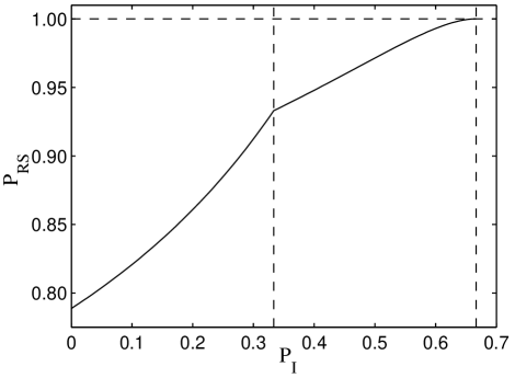
Figure 3: Dependence of the relative success rate, $P_{RS}$, on the probability of inconclusive results, $P_{I}$, for optimal universal multimeter with program $|\psi_{+}\rangle|\psi_{-}\rangle$.

At this stage we are ready to write down the total success rate and inconclusive-result rate for the discrimination of states $R_{\pm}$. Clearly,

$$P_{S}=\frac{1}{3}P^{\prime\prime}_{S}+\frac{2}{3}P^{\prime}_{S},\qquad P_{I}=\frac{1}{3}P^{\prime\prime}_{I}+\frac{2}{3}P^{\prime}_{I}.$$

We can also introduce the relative success rate (i.e., the success rate calculated only for “conclusive” results): $P_{RS}={P_{S}}/{(1-P_{I})}$.

One must examine four different sets of parameter $a$: $a\in[0,\frac{1}{2})$, $a=\frac{1}{2}$, $a\in(\frac{1}{2},\frac{1}{2}(1+\frac{1}{\sqrt{3}})]$, and $a\in(\frac{1}{2}(1+\frac{1}{\sqrt{3}}),1]$. Finally, it can be seen that (see also Fig. 3)

$$P_{S}=\left\{\begin{array}[]{lll}\displaystyle\frac{1}{2}\left(1+\frac{1}{\sqrt{3}}\right)-\frac{P_{I}}{2}&\mbox{~{}~{}if~{}~{}}&\displaystyle 0\leq P_{I}\leq\frac{1}{3},\\[11.38109pt] \displaystyle\frac{1}{2}-\frac{P_{I}}{2}+\frac{1}{3}\sqrt{\frac{5}{4}-\frac{3P_{I}}{2}}&\mbox{~{}~{}if~{}~{}}&\displaystyle\frac{1}{3}<P_{I}\leq\frac{2}{3}.\end{array}\right.$$ (49)

For $P_{I}=2/3$ the error-free operation ($P_{RS}=1$) is approached and further increasing of $P_{I}$ has no reason.

Apparently, the optimal POVM for universal multimeters with fixed fraction of inconclusive results has two different forms according to the value of the probability of inconclusive result. First let us write down the POVM for $P_{I}\in[0,\frac{1}{3}]$:

$$\Pi_{\pm} = \Pi^{\mathrm{D}}_{\pm}-\frac{3}{2}P_{I}\,\Pi_{\mathrm{sym}},$$

$$\Pi_{?} = 3P_{I}\,\Pi_{\mathrm{sym}},$$ (50)

where $\Pi^{\mathrm{D}}_{\pm}$ denote the elements of POVM for deterministic discrimination that are defined by Eq. (42).

When $P_{I}\in(\frac{1}{3},\frac{2}{3}]$ the POVM can be expressed as

$$\Pi_{\pm} = \Pi_{\pm,A}+\Pi_{\pm,B},$$

$$\Pi_{?} = \Pi_{\mathrm{sym}}+\Pi_{?,A}+\Pi_{?,B},$$ (51)

where $\Pi_{\pm,B}$ and $\Pi_{?,B}$ are POVM elements for discrimination of vectors $|B_{\pm}\rangle$ that can be obtained in a completely analogous way as that for vectors $|A_{\pm}\rangle$ [see Eq. (45)]. For $P_{I}=\frac{1}{3}$ the two POVM (50) and (51) coincide [notice, that for $\Phi=45^{\circ}$, $|\Xi_{+}\rangle=-|\phi_{2}\rangle$ as follows from Eqs. (43) and (46)].

The operation of the multimeter for different values of $P_{I}$ can be figured as follows: When $P_{I}$ grows from zero it is the most convenient to gradually move the contributions, that are the same for both $R_{\pm}$ and that substantially contribute to errors, from conclusive to inconclusive results. It means the multiple of the projector to the symmetric subspace increases in $\Pi_{?}$. When $P_{I}=1/3$ then $\Pi_{?}=\Pi_{\mathrm{sym}}$ and further increase of the fraction of $\Pi_{\mathrm{sym}}$ is impossible (because $\Pi_{\pm}$ and $\Pi_{?}$ must form a POVM). If one wants to increase $P_{I}$ further above $1/3$ he/she must start to turn vectors $|\Xi_{\pm}\rangle$ as described above. The point $P_{I}=2/3$ corresponds to the unambiguous discrimination.

IV Universal probabilistic error-free multimeter for qudits

Let us consider a multimeter that could realize an arbitrary von-Neumann projective measurement on a single $d$-level system (qudit). Let $|\psi_{j}\rangle$, $j=1,\ldots,d$ denote orthonormal-basis states. We consider the conceptually simplest program that consists of the $d$ qudits in basis states,

$$|\Psi\rangle_{\mathrm{p}} = |\psi_{1}\rangle|\psi_{2}\rangle\ldots|\psi_{j}\rangle\ldots|\psi_{d}\rangle\equiv[U_{d}(g)]^{\otimes d}|\Psi_{0}\rangle_{\mathrm{p}},$$

where $|\Psi_{0}\rangle_{\mathrm{p}}=|1\rangle|2\rangle\ldots|j\rangle\ldots|d\rangle$, $U_{d}(g)$ is a unitary operation acting on the basis states according to $U_{d}(g)|j\rangle=|\psi_{j}\rangle$ and $g\in SU(d)$. We are interested in the probabilistic error-free multimeter that can respond with an inconclusive outcome but it never makes an error, i.e. $\pi_{j}\propto|\psi_{j}\rangle\langle\psi_{j}|$. The multimeter is described by a $(d+1)$-component POVM on $d+1$ qudits (the data qudit and $d$ program qudits). The POVM $\{\Pi_{1},\ldots,\Pi_{d},\Pi_{?}\}$ should optimally unambiguously discriminate among $d$ mixed states

$$R_{j} = \int_{SU(d)}U_{d}(g)|j\rangle_{\mathrm{data}}\langle j|U_{d}^{\dagger}(g)$$ (52)

$$\otimes[U_{d}(g)]^{\otimes d}|\Psi_{0}\rangle_{\mathrm{p}}\langle\Psi_{0}|[U_{d}^{\dagger}(g)]^{\otimes d}d\mu(g),$$

where the integration is carried over the whole group $SU(d)$ with the invariant Haar measure $d\mu(g)$.

We conjecture that the optimal POVM elements $\Pi_{j}$ have the following structure

$$\Pi_{j} = C\,|\Sigma_{d}^{-}\rangle_{\bar{j}}\langle\Sigma_{d}^{-}|\otimes\openone_{j},$$

$$\Pi_{?} = \openone-\sum_{j=1}^{d}\Pi_{j},$$ (53)

where $|\Sigma_{d}^{-}\rangle_{\bar{j}}$ is totally antisymmetric state of $d$ qudits: the data qudit and all program qudits except for the $j$-th qudit, and $\openone_{j}$ stands for the identity operator on the Hilbert space of the $j$-th program qudit. We can write

$$|\Sigma_{d}^{-}\rangle_{\bar{j}}=\frac{1}{\sqrt{d!}}\sum_{\bm{i}}\epsilon_{\bm{i}}|i_{1}\rangle_{\mathrm{data}}\otimes|i_{2},\ldots,i_{d}\rangle_{\mathrm{p}\bar{j}},$$ (54)

where we sum over all permutations of $\{1,2,\ldots,d\}$ and $\epsilon_{\bm{i}}$ is the sign of the permutation. Apparently, vectors $|\Sigma_{d}^{-}\rangle_{\bar{j}}\otimes|x\rangle_{j}$, where $|x\rangle_{j}$ is an arbitrary state of the $j$-th program qudit, are orthogonal to any vector $|\Psi_{k}\rangle=|\psi_{k}\rangle_{\mathrm{data}}|\psi_{1}\rangle|\psi_{2}\rangle\dots|\psi_{d}\rangle$ with $k\neq j$. It is easy to verify that $\mathrm{Tr}[\Pi_{j}R_{k}]\propto\delta_{jk}$. It means, the only contribution to the outcome $\Pi_{j}$ can originate from the $j$-th basis state of the data qudit.

Clearly, POVM (53) is the POVM describing a probabilistic unambiguous multimeter. We believe it is even the optimal one. This hypothesis is based on the conjecture that the kernels of operators $R_{j}$ have the form $\mathcal{K}_{j}=\mathcal{H}^{\mathrm{ant}}_{j}\otimes\openone_{\bar{j}}$ where $\mathcal{H}^{\mathrm{ant}}_{j}$ is the antisymmetric space of two qudits — the data one and $j$-th program one. Symbol $\openone_{\bar{j}}$ denotes identity operator on $d-1$ program qudits exclusive of $j$-th qudit. (At worst, $\mathcal{K}_{j}$ are the subspaces of the appropriate kernels.) The $d$-dimensional subspace spanned by $|\Sigma_{d}^{-}\rangle_{\bar{j}}\otimes|x\rangle_{j}$, where $|x\rangle_{j}$ is an arbitrary state of the $j$-th qudit, represents an intersection of $d-1$ spaces $\mathcal{K}_{k}$ (excluding the $j$-th one): $\bigcap_{\begin{subarray}{c}k=1\\ k\neq j\end{subarray}}^{d}\mathcal{K}_{k}$.

The sum of the $d$ POVM elements $\Pi_{j}$ must be lower than the identity operator, $\sum_{j=1}^{d}\Pi_{j}\leq\openone,$ which imposes a constraint on the normalization factor $C$. Since we want to maximize the probability of success we must choose the maximum possible $C$, which can be expressed in terms of the maximum eigenvalue of the operator

$$Y=\sum_{j=1}^{d}|\Sigma_{d}^{-}\rangle_{\bar{j}}\langle\Sigma_{d}^{-}|\otimes\openone_{j}.$$

The maximal admissible $C$ reads

$$C=\{\max[\mathrm{eig}(Y)]\}^{-1}.$$ (55)

Instead of looking for the maximum eigenvalue of $Y$ we can equivalently calculate the maximum eigenvalue of the operator

$$Z=\sum_{j=1}^{d}|f_{j}\rangle\langle f_{j}|,$$ (56)

where $|f_{j}\rangle=|\Sigma_{d}^{-}\rangle_{\bar{j}}|1\rangle_{j}$. The $d$ linearly independent states $|f_{j}\rangle$ span a $d$-dimensional Hilbert space $\mathcal{H}_{f}$. We can write $|f_{j}\rangle=M|e_{j}\rangle$ where $|e_{j}\rangle$ form an orthonormal basis in $\mathcal{H}_{f}$. On inserting this expression into Eq. (56) we find that

$$Z=\sum_{j=1}^{d}M|e_{j}\rangle\langle e_{j}|M^{\dagger}=MM^{\dagger},$$ (57)

where the completeness of the basis $|e_{j}\rangle$ on $\mathcal{H}_{f}$ has been used. It holds for any square matrix $M$ that $MM^{\dagger}$ has the same eigenvalues as $F=M^{\dagger}M$. In the basis $|e_{j}\rangle$ the matrix elements of $F$ read $F_{jk}=\langle f_{j}|f_{k}\rangle$. We thus have to determine the scalar products of the non-orthogonal states $|f_{j}\rangle$. Let us introduce unnormalized states of $d-1$ qudits, $|\sigma_{d-1}^{-}\rangle_{\bar{j}\bar{k}}$, that are obtained by projecting the $k$-th program qudit of the state $|\Sigma_{d}^{-}\rangle_{\bar{j}}$ onto state $|1\rangle_{k}$. It follows that $F_{jk}$ can be calculated as a scalar product of $|\sigma_{d-1}^{-}\rangle_{\bar{j}\bar{k}}$ and $|\sigma_{d-1}^{-}\rangle_{\bar{k}\bar{j}}$,

$$F_{jk}=\,_{\bar{j}\bar{k}}\langle\sigma_{d-1}^{-}|\sigma_{d-1}^{-}\rangle_{\bar{k}\bar{j}}$$ (58)

It is easy to deduce from the Slater determinant representation of the totally antisymmetric state (54) that also $|\sigma_{d-1}^{-}\rangle_{\bar{j}\bar{k}}$ is a totally antisymmetric state of the data qudit and all the program qudits except $j$-th and $k$-th ones,

$$|\sigma_{d-1}^{-}\rangle_{\bar{j}\bar{k}}=\frac{(-1)^{t}}{\sqrt{d!}}\sum_{\bm{i}}\epsilon^{\prime}_{\bm{i}}|i_{1}\rangle_{\mathrm{data}}\otimes|i_{2},\ldots,i_{d-1}\rangle_{\mathrm{p},\bar{j}\bar{k}},$$ (59)

where one sums over all permutations of $\{2,3,\ldots,d\}$, $\epsilon^{\prime}_{\bm{i}}$ is the sign of the permutation, and

$$t=\left\{\begin{array}[]{lll}k&\mbox{~{}for~{}}&j>k,\\ k-1&\mbox{~{}for~{}}&j<k.\end{array}\right.$$

Assuming $j\neq k$ and inserting the expressions (59) into Eq. (58) we immediately find that

$$F_{jk}=\frac{(d-1)!}{d!}(-1)^{j+k-1},\qquad j\neq k.$$ (60)

Since $|f_{j}\rangle$ are normalized we finally have

$$F_{jk}=\delta_{jk}+(1-\delta_{jk})\frac{(-1)^{j+k-1}}{d}.$$ (61)

The operator $F$ can be easily diagonalized,

$$F=\left(1+\frac{1}{d}\right)\openone-|\varphi_{d}\rangle\langle\varphi_{d}|,$$ (62)

where $|\varphi_{d}\rangle=\frac{1}{\sqrt{d}}\sum_{j=1}^{d}(-1)^{j}|e_{j}\rangle$. It follows from (62) that the largest eigenvalue of $F$ is $\mu_{\mathrm{max}}=1+1/d$ hence $C=d/(d+1)$ and the normalized POVM (53) reads,

$$\Pi_{j}=\frac{d}{d+1}\,|\Sigma_{d}^{-}\rangle_{\bar{j}}\langle\Sigma_{d}^{-}|\otimes\openone_{j}.$$ (63)

By construction, the probabilistic multimeter is universal and the probability of success

$$P_{S}=\frac{d}{(d+1)!}$$ (64)

does not depend on the particular basis chosen by the program state and on the basis state $|\psi_{j}\rangle$ sent to the data register. Consequently the multimeter indeed probabilistically implements the projective measurement in the basis $\{|\psi_{j}\rangle\}_{j=1}^{d}$ and the effective POVM on the data qudit reads

$$\pi_{j} = P_{S}\,|\psi_{j}\rangle\langle\psi_{j}|,\qquad j=1,\ldots,d,$$

$$\pi_{?} = (1-P_{S})\openone.$$ (65)

V Conclusions

In this paper we have investigated a broad class of quantum multimeters that can perform a projective measurement on a single data qubit (or qudit). The main feature of the quantum multimeters is that the measurement basis is controlled by the quantum state of the program register that serves as a kind of a quantum “software” while the multimeter itself (a quantum “hardware”) performs a fixed joint measurement on the data and program states.

In our investigations we have assumed finite-dimensional program register, typically consisting of several qubits (or qudits). In this case it is impossible to design perfect multimeter that would perform exactly and deterministically the projective measurement in any basis from a continuous set, with the basis being determined by the state of the program register. The multimeters designed here are therefore only approximate. Two conceptually different approximations have been considered. In the first case, the multimeter operates deterministically and always produces an outcome but the effective measurement on the data deviates from the ideal projective measurement. Such errors are avoided in the second approach when the multimeter is a probabilistic device whose operation sometimes fails but, when it succeeds, then it carries out exactly the desired projective measurement.

We have demonstrated that these two kinds of multimeters are in fact just limit cases from a whole class of probabilistic multimeters that are characterized by a certain fraction $P_{I}$ of the inconclusive results. For a fixed dependence of the program on the measurement basis, the problem of designing the optimal multimeter is formally equivalent to finding the optimal POVM for discrimination of two mixed states. With the help of the recently developed theory of optimal probabilistic discrimination of mixed quantum states we have been able to analytically determine the optimal phase-covariant multimeter for $N$-qubit program $|\psi_{+}\rangle^{\otimes N}$ as well as a universal multimeter with a two-qubit program $|\psi_{+}\rangle|\psi_{-}\rangle$. Remarkably, in both cases the success rate of the optimal deterministic multimeter exactly coincides with the optimal fidelity of estimation of the basis state $|\psi_{+}\rangle$ from a single copy of the program state.

We have also proposed a generalization of the probabilistic error-free multimeter to qudits assuming that the $d$-qudit program consists of a product of the $d$ basis states. The construction of this multimeter is inspired by the structure of the optimal probabilistic multimeter for qubits and relies on projections on totally anti-symmetric state of $d$ qudits.

Our findings clearly illustrate that the measurement on the data qubit can be quite efficiently controlled by the quantum state of the program register. In particular, we emphasize that a classical description of the measurement basis would require infinitely many bits of classical information, while only a few quantum bits suffice in the present case to obtain an error-free (although probabilistic) operation. Our results also reveal many intriguing connections between the concept of quantum multimeters, discrimination of quantum states and optimal quantum state estimation. This suggests that there might be also links to the related problems of transmitting information about the direction in space Bagan00 ; Peres01a ; Bagan01a or about the reference frame Peres01b ; Bagan01b using the quantum states. For instance, it is well known that the use of entangled states can improve the fidelity of transmission in the two latter cases. A natural question arises whether using entangled states as programs one could achieve higher success rate (for a fixed size of the program register) than with the product-state programs considered in the present paper. More generally, one would ultimately like to know what is the optimal program leading to maximal achievable success rate. This is a highly nontrivial optimization problem that certainly deserves further investigation.

References

• (1) M. Dušek and V. Bužek, Phys. Rev. A 66, 022112 (2002).
• (2) J. Fiurášek, M. Dušek and R. Filip, Phys. Rev. Lett. 89, 190401 (2002); J. Fiurášek, M. Dušek and R. Filip, Fortschritte der Physik 51, 107 (2003).
• (3) M. A. Nielsen and I. L. Chuang, Phys. Rev. Lett. 79, 321 (1997).
• (4) G. Vidal, L. Masanes, and J. I. Cirac, Phys. Rev. Lett. 88, 047905 (2002).
• (5) M. Hillery V. Bužek, and M. Ziman, Phys. Rev. A 65, 022301 (2002).
• (6) M. Hillery, M. Ziman, and V. Bužek, Phys. Rev. A 66, 042302 (2002).
• (7) J. P. Paz and A. Roncaglia, quant-ph/0306143.
• (8) M. Sasaki and A. Carlini, Phys. Rev. A 66, 022303 (2002).
• (9) S. M. Barnett, A. Chefles, and I. Jex, Phys. Lett. A 307, 189 (2003).
• (10) G. M. D’Ariano, P. Perinotti, M. F. Sacchi, quant-ph/0306025.
• (11) C. W. Helstrom, Quantum Detection and Estimation Theory Academic Press, New York, 1976).
• (12) R. Derka, V. Bužek, and A.  K. Ekert Phys. Rev. Lett. 80, 1571 (1998).
• (13) T. Rudolph, R. W. Spekkens, and P. S. Turner, Phys. Rev. A 68, 010301 (2003).
• (14) P. Raynal, N. Lütkenhaus, and S. J. van Enk, Phys. Rev. A 68, 022308 (2003).
• (15) J. Fiurášek and M. Ježek, Phys. Rev. A 67, 012321 (2003).
• (16) Y. C. Eldar, Phys. Rev. A 67, 042309 (2003).
• (17) I. D. Ivanovic, Phys. Lett. A 123, 257 (1987).
• (18) D. Dieks, Phys. Lett. A 126, 303 (1988).
• (19) A. Peres, Phys. Lett. A 128, 19 (1988).
• (20) G. M. D’Ariano and C. Macchiavello, Phys. Rev. A 67, 042306 (2003).
• (21) A. Chefles and S. M. Barnett, J. Mod. Opt. 45, 1295 (1998).
• (22) C. W. Zhang, C. F. Li, and G. C. Guo, Phys. Lett. A 261, 25 (1999).
• (23) E. Bagan, M. Baig, A. Brey, R. Muñoz-Tapia, and R. Tarrach Phys. Rev. Lett. 85, 5230 (2000).
• (24) A. Peres and P. F. Scudo, Phys. Rev. Lett. 86, 4160 (2001).
• (25) E. Bagan, M. Baig, A. Brey, R. Muñoz-Tapia, and R. Tarrach, Phys. Rev. A 63, 052309 (2001).
• (26) A. Peres and P. F. Scudo, Phys. Rev. Lett. 87, 167901 (2001).
• (27) E. Bagan, M. Baig, and R. Muñoz-Tapia, Phys. Rev. Lett. 87, 257903 (2001).