Quantum information via state partitions and the context translation principle

Abstract

For many–particle systems, quantum information in base $n$ can be defined by partitioning the set of states according to the outcomes of $n$–ary (joint) observables. Thereby, $k$ particles can carry $k$ nits. With regards to the randomness of single outcomes, a context translation principle is proposed. Quantum randomness is related to the uncontrollable degrees of freedom of the measurement interface, thereby translating a mismatch between the state prepared and the state measured.

1 Information in many–particle quantum systems

The preparation of a single particle $n$–state quantum system in a single state constitutes the operationalization of a nit, or qunit. Likewise, the occurrence of an outcome of an observable with $n$ possible outcomes can be associated with accessing a nit of information. For a single particle observable, this is associated with choosing a vector from an orthogonal basis of $n$–dimensional Hilbert space. In the many–particle case, nits may not only be localized at single particle observables, since due to entanglement, the nits may be distributed over the particles by representing joint particle properties.

In what follows we shall review and extend formal generalizations [1, 2] of the single particle two–state case to an arbitrary finite number of particles with an arbitrary finite number of different measurement outcomes per particle. Thereby, we define a nit as a radix $n$ measure of quantum information which is based on state partitions associated with the outcomes of $n$–ary observables. We shall demonstrate the following property: $k$ particles specify $k$ nits in such a way that $k$ measurements of comeasurable observables with $n$ possible outcomes are necessary to determine the information. Stated pointedly, $k$ particles can carry $k$ nits.

Conceptually, such properties have been previously proposed by Zeilinger [3] as a foundational principle for quantum mechanics. Zeilinger merely considered two–state systems of two and three particles, yet an informal hint for higher–dimensional single quantum systems is in footnote 6 of [3, p. 635]. There is a slight difference in the approach of Zeilinger and the author: whereas here the logico–algebraic properties are studied ‘top-down’ by assuming Hilbert space quantum mechanics and arriving at the foundational principle purely deductively, Zeilinger and Brukner [4] reconstruct certain features of quantum physics by treating this principle ‘bottom–up’ as an axiom.

1.1 Definition

For a single $n$–state particle, the nit can be formalized as a fine-grained partition of $n$ orthogonal states; i.e., if the set of orthogonal states is represented by $\{1,\ldots,n\}$, then the nit is defined by choosing one element of the set $\{\{1\},\ldots,\{n\}\}$.

The generalization to $k$ particles involves the construction of $k$ partitions of the product states with $n$ elements per partition in such a way that every single product state is obtained by the set theoretic intersection of $k$ elements of all the different partitions. That is, the partitions which properly represent the set of nits have to be defined to obey the following properties: (i) every set theoretic intersection of single elements of the $k$ partitions, one element per partition, yields a single product state, and (ii) the union of all these intersections obtained by (i) is just the set of product states. Every single such partition can be interpreted as a nit. For their implementation, we shall adopt an $n$–ary search strategy.

In the following, the standard orthonormal basis of $n^{k}$–dimensional Hilbert space is identified with the set of states $S=\{1,2,\ldots,n^{k}\}$; i.e., (superscript ‘$T$’ indicates transposition) $1\equiv(1,\ldots,0)^{T}\equiv\mid 1_{1},\ldots,1_{k}\rangle=\mid 1_{1}\rangle\otimes\cdots\otimes\mid 1_{k}\rangle$, $\ldots$, $n^{k}\equiv(0,\ldots,1)^{T}\equiv\mid n_{1},\ldots,n_{k}\rangle$. Here, the single particle states are labelled by $1_{1}$ through $n_{k}$, respectively. Tensor product states are formed and ordered lexicographically ($0<1$).

The nit operators are defined via diagonal matrices which contain $n^{k-1}$ equal amounts of $n$ mutually different numbers such as different primes $q_{1},\ldots,q_{n}$; i.e.,

$$\begin{array}[]{llll}F_{1}&=&{\rm diag}(\underbrace{\underbrace{q_{1},\ldots,q_{1}}_{n^{k-1}\;{\rm times}},\ldots,\underbrace{q_{n},\ldots,q_{n}}_{n^{k-1}\;{\rm times}}}_{n^{0}=1\;{\rm times}}),\\ F_{2}&=&{\rm diag}(\underbrace{\underbrace{q_{1},\ldots,q_{1}}_{n^{k-2}\;{\rm times}},\ldots,\underbrace{q_{n},\ldots,q_{n}}_{n^{k-2}\;{\rm times}}}_{n^{1}\;{\rm times}}),\\ &\vdots&\\ F_{k}&=&{\rm diag}(\underbrace{q_{1},\ldots,q_{n}}_{n^{k-1}\;{\rm times}}).\end{array}$$ (1)

‘${\rm diag}(a,b,\ldots)$’ stands for the diagonal matrix with $a,b,\ldots$ at the diagonal entries. The operators implement an $n$–ary search filter, separating the search space into $n$ equal partitions of states, such that successive applications of all such filters renders a single state. In this simplest, nonentangled, case, the meaning of the $i$’th filter or nit operator $F_{i}$, $1\leq i\leq k$, can be expressed as the proposition, ‘the $i$’th particle is in state $q_{1},\ldots,q_{n}$.’ The nit operators in equation (1) can be combined to a single measurement. The corresponding ‘context operator’ $C=F_{1}F_{2}\cdots F_{k}$ can be obtained by taking different prime numbers as diagonal entries of $F_{1},\ldots,F_{k}$ (cf. examples below).

There exist $n^{k}!$ sets of nit operators, which are obtained by forming a $(k\times n^{k})$–matrix

$$\left(\begin{array}[]{ccccccccccccccccccccc}q_{1}&\ldots&q_{1}&\ldots&q_{n}&\ldots&q_{n}\\ &&&\ldots&&&\\ q_{1}&\ldots&q_{n}&\ldots&q_{1}&\ldots&q_{n}\end{array}\right)$$ (2)

whose rows are the diagonal components of $F_{1},\ldots,F_{k}$ from equation  (1), by permuting its columns, and finally by reinterpreting the rows as the diagonal entries of the new nit operators $F_{1}^{\prime},\ldots,F_{k}^{\prime}$. This formal procedure is equivalent to permuting (the labels of) the $n^{k}$ product states. One consequence of the rearrangement is the transition from nonentangled eigenstates of the single particle states to entangled eigenstates thereof (see example below). No straightforward meaning could be associated to the new nit operators in this general case. Note that all partitions discussed so far are equally weighted and well balanced, as all elements of them contain an equal number of states.

1.2 Examples: two three–state particle cases and entanglement

An example for the two three–state particle case has been enumerated in Ref. [2]. Recall that, in the simplest case, the two nit operators can be constructed according to the scheme in equation (1) and represented by

$$\begin{array}[]{llllll}F_{1}&=&\{\{1,2,3\},\{4,5,6\},\{7,8,9\}\}&\equiv&{\rm diag}(a,a,a,b,b,b,c,c,c),\\ F_{2}&=&\{\{1,4,7\},\{2,5,8\},\{3,6,9\}\}&\equiv&{\rm diag}(a,b,c,a,b,c,a,b,c).\\ \end{array}$$ (3)

If, on the other hand, $F_{2}={\rm diag}(d,e,f,d,e,f,d,e,f)$ and $a,b,c,d,e,f,$ are six different prime numbers, then, due to the uniqueness of prime decompositions, the two trit operators can be combined to a single context operator

$$C=F_{1}\cdot F_{2}=F_{2}\cdot F_{1}={\rm diag}(ad,ae,af,bd,be,bf,cd,ce,cf)$$ (4)

which acts on both particles. As $C$ has nine different eigenvalues, it separates the nine product states completely and at once.

Just as for the two states per particle case [1], there exist $3^{2}!=9!=362880$ permutations of operators which are all able to separate the nine states. According to equation (2), they are obtained by forming a $(2\times 9)$–matrix whose rows are the diagonal components of $F_{1}$ and $F_{2}$ from equation (3) and permuting all the columns. The resulting new operators are also valid trit operators; i.e., for every one of the new pair of partitions (i) the set theoretic intersection of single elements of the two partitions, one element per partition, is a single product state, and (ii) the union of all these intersections obtained by (i) is just the set of product states. (For a proof recall that every permutation amounts to a relabelling the product states.)

The complete set of $9!/(2\cdot 3!\cdot 3!)=5040$ different two–trit sets can be evaluated numerically; i.e., in lexicographic order,

$$\{\{\{\{1,2,3\},\{4,6,8\},\{5,7,9\}\}\times\{\{1,4,5\},\{2,6,7\},\{3,8,9\}\}\},$$ (5)

$$\{\{\{1,2,3\},\{4,6,9\},\{5,7,8\}\}\times\{\{1,4,5\},\{2,6,7\},\{3,8,9\}\}\},$$ (6)

$$\vdots$$

$$\{\{\{1,5,9\},\{2,6,7\},\{3,4,8\}\}\times\{\{\{1,6,8\},\{2,4,9\},\{3,5,7\}\}\},$$ (7)

$$\vdots$$

$$\{\{\{1,6,9\},\{2,5,7\},\{3,4,8\}\}\times\{\{1,7,8\},\{2,4,9\},\{3,5,6\}\}\},$$ (8)

$$\{\{\{1,6,9\},\{2,5,8\},\{3,4,7\}\}\times\{\{1,7,8\},\{2,4,9\},\{3,5,6\}\}\}\}.$$ (9)

A graphical representation of the single particle state space tesselation is depicted in figure 1.

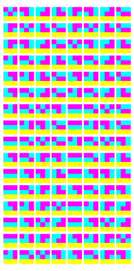
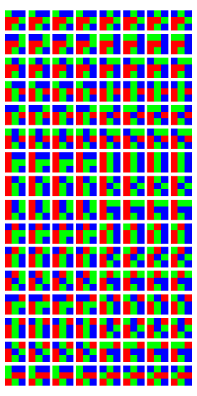
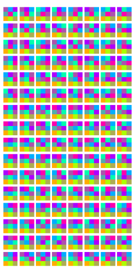
trit 1	trit 2	trits 1&2

Figure 1: Two trits yield a unique tessellation of the two particle product state space. The first and second single particle states are drawn horizontally and vertically, respectively. Depicted are the first cases of equations (5)—(9).

In general, the permutations transform nonentangled states into entangled ones. Consider, for the sake of detail, the ‘(counter)diagonal’ set of trits listed in equation  (7), which is induced by the permutation whose cycle form is (1)(2,5,6,7,3,9,8,4). If the same two particle $(3\times 3)$ product state space representation is used as in figure 1, then the trits just correspond to the completed diagonals and counterdiagonals; i.e., if the single particle states are labelled by $a_{1},b_{1},c_{1}$ and $a_{2},b_{2},c_{2}$, respectively, then the new trit eigenstates $\{|\psi_{1}\rangle,|\psi_{2}\rangle,|\psi_{3}\rangle\}$ and $\{|\psi_{4}\rangle,|\psi_{5}\rangle,|\psi_{6}\rangle\}$ are

$$\begin{array}[]{llllll}|\psi_{1}\rangle&=&\frac{1}{\sqrt{3}}\left(|a_{1}a_{2}\rangle+|b_{1}b_{2}\rangle+|c_{1}c_{2}\rangle\right)\equiv\frac{1}{\sqrt{3}}\left(1,0,0,0,1,0,0,0,1\right)^{T},\\ &\vdots&\\ |\psi_{6}\rangle&=&\frac{1}{\sqrt{3}}\left(|c_{1}a_{2}\rangle+|b_{1}b_{2}\rangle+|a_{1}c_{2}\rangle\right)\equiv\frac{1}{\sqrt{3}}\left(0,0,1,0,1,0,1,0,0\right)^{T}.\end{array}$$ (10)

The associated trit operators are representable by $F_{1}={\rm diag}(a,c,b,b,a,c,c,b,a)$ and $F_{2}={\rm diag}(d,e,f,e,f,d,f,d,e)$, respectively; with different $a=d$, $c=e$, and $b=f$; or, alternatively, with mutually different numbers $a,b,c,d,e,f$. With respect to the original single particle states, the trit eigenstates (10) are entangled.

1.3 Inverse problems

Consider the related dual or inverse problem: suppose that a complete set of orthonormal states $S^{\prime}$ is given; what is the minimal set of comeasurable queries necessary to separate any single one of these states from the other ones? To answer this question, the unitary transformation $U$ connecting the set of orthogonal states $S^{\prime}$ with the standard orthonormal Cartesian basis $S$ can be used to transform the nit operators in equation (1) into their appropriate form.

For two-state systems labelled by ‘$+$’ and ‘$-$,’ the method can for instance be applied to a set of orthonormal base states of eight dimensional Hilbert space which contains the W–state introduced in [5] and discussed in [6].

$$\begin{array}[]{lll}&&|\phi_{1}\rangle=|+++\rangle\\ &&|\phi_{2}\rangle=\frac{1}{\sqrt{3}}\left(|++-\rangle+|+-+\rangle+|-++\rangle\right)\\ &&|\phi_{3}\rangle=\frac{1}{\sqrt{2}}\left(-|++-\rangle+|-++\rangle\right)\\ &&|\phi_{4}\rangle=\frac{1}{\sqrt{6}}\left(-|++-\rangle+2|+-+\rangle-|-++\rangle\right)\\ &&|\phi_{5}\rangle=\frac{1}{\sqrt{3}}\left(|+--\rangle+|-+-\rangle+|--+\rangle\right)\\ &&|\phi_{6}\rangle=\frac{1}{\sqrt{2}}\left(-|+--\rangle+|--+\rangle\right)\\ &&|\phi_{7}\rangle=\frac{1}{\sqrt{6}}\left(-|+--\rangle+2|-+-\rangle-|--+\rangle\right)\\ &&|\phi_{8}\rangle=|---\rangle\end{array}$$ (19)

Consider the unitary transformation $U^{\textrm{W}}$ given by

$$U^{\textrm{W}}=\left(\begin{array}[]{rrrrrrrr}1&0&0&0&0&0&0&0\\ 0&\frac{1}{{\sqrt{3}}}&-\frac{1}{{\sqrt{2}}}&-\frac{1}{{\sqrt{6}}}&0&0&0&0\\ 0&\frac{1}{{\sqrt{3}}}&0&\frac{2}{{\sqrt{6}}}&0&0&0&0\\ 0&\frac{1}{{\sqrt{3}}}&\frac{1}{{\sqrt{2}}}&-\frac{1}{{\sqrt{6}}}&0&0&0&0\\ 0&0&0&0&\frac{1}{{\sqrt{3}}}&-\frac{1}{{\sqrt{2}}}&-\frac{1}{{\sqrt{6}}}&0\\ 0&0&0&0&\frac{1}{{\sqrt{3}}}&0&\frac{2}{{\sqrt{6}}}&0\\ 0&0&0&0&\frac{1}{{\sqrt{3}}}&\frac{1}{{\sqrt{2}}}&-\frac{1}{{\sqrt{6}}}&0\\ 0&0&0&0&0&0&0&1\\ \end{array}\right).$$ (20)

By construction, when applied to the vectors of the standard orthonormal Cartesian basis, $U^{\textrm{W}}$ yields the states enumerated in equation (19). The corresponding bit operators $F_{1}$, $F_{2}$, $F_{3}$ and the context operator $C$ are

$$\begin{array}[]{lll}F_{1}&=&U^{\textrm{W}}\cdot\textrm{diag}\left(2,2,2,2,3,3,3,3\right)\cdot{U^{\textrm{W}}}^{\dagger}=\textrm{diag}\left(2,2,2,2,3,3,3,3\right),\\ F_{2}&=&U^{\textrm{W}}\cdot\textrm{diag}\left(5,5,7,7,5,5,7,7\right)\cdot{U^{\textrm{W}}}^{\dagger},\\ F_{3}&=&U^{\textrm{W}}\cdot\textrm{diag}\left(11,13,11,13,11,13,11,13\right)\cdot{U^{\textrm{W}}}^{\dagger},\\ C&=&F_{1}F_{2}F_{3}=U^{\textrm{W}}\cdot\textrm{diag}\left(110,130,154,182,165,195,231,273\right)\cdot{U^{\textrm{W}}}^{\dagger}.\end{array}$$ (21)

Note that, if instead of the prime numbers 2, 5, 11 and 3, 7, 13, we would have used 1 and 0, respectively, projection operators would have resulted, but this strategy can only be applied to the binary case [1].

2 Information of single quantum systems

Having defined nits for the many–particle case, let us now turn our attention to ome of the mysterious and puzzling issues of quantum mechanics: the postulated randomness of certain measurement outcomes introduces an irreducible element of acausality. Quantum randomness is accompanied by other principal limits of operationalization and rational decidability, such as complementarity and contextuality. Encouraged by the conference agenda and by many inspiring discussions with Professor Greenberger, I shall raise a speculative and even controversial topic and explore the randomness encountered in single and many–particle quantum systems when there is a nit mismatch between the states prepared and the states measured.

2.1 Amazing single particle quantum systems

Consider simple quantum mechanical preparation procedures, such as the preparation of electrons in pure spin states along a particular direction realizable by a Stern–Gerlach device. Let us assume that we have prepared or ‘programmed’ the electron spin to be in the ‘up’ state along our $z$–axis. Then, by convincing ourselves that, when measured along $z$, the electron spin is always ‘up,’ we decide to ask the electron a ‘complementary’ question, such as, “what is the direction of spin along the $x$–axis perpendicular to the $z$–axis?’ According to the quantum canon, in particular quantum complementarity, the electron is totally incapable of ‘storing’ precisely more than one bit of information about its spin state in a single direction; in particular it does not store a second bit of information about its spin state in any perpendicular direction thereof. So, when interrogated about issues it was not at all prepared to answer, it is at a complete loss of providing such information.

In this respect, the electron is like an input/output automaton accepting only sequences of strings consisting of the symbol ‘$a$,’ being confronted with the symbol ‘$b$.’ Indeed, to ridiculously overextend the ‘Copenhagen interpretation’ to this automaton case, it would not make much sense to push the word ‘$ab$’ onto the automaton and watch its behaviour, since such a behaviour property does not exist. The query seems to be an absurd one in the sense of nonexistence of these properties.

Hence, quantum analogies with deterministic agents seem to end when considering what happens in the case of absurd queries. Deterministic agents are incapable of handling improper input, on which they offer no answer at all. The electron, on the contrary, seems to provide an answer, albeit an irreducibly random one. (In this case it behaves just like most Viennese when asked about a location they do not know: they are too embarrassed to confess their ignorance, so they will send the questioner off into arbitrary directions;)

Thus, from the computational point of view, electrons are amazing little gadgets: they are incapable of adding two plus two, let alone universal computation; yet in terms of algorithmic information theory [7, 8], any humble electron seems to possess super–Turing computation powers. To be more precise: according to the ‘creed’ canonized by some ‘quantum council,’ the occurrence of certain individual quantum events are believed to be totally unpredictable, unlawful, acausal, and thus independent of past, present and future states of the system and of its surroundings, such as the measurement interface, in any algorithmically meaningful way . As a consequence, with high probability, algorithmically incompressible sequences can be generated from quantum coin tosses [9, 10]. Summing up, in terms of spin, electrons seem to specialize in two antithetical tasks, and in nothing else: being prepared to issue a deterministic answer when asked a proper question; and tossing more or less fair coins if asked improper questions.

2.2 Quantum randomness through context translation

We propose that the discrepancies of the seemingly inconsistent computational powers of single quantum systems, such as the electron spin, can be overcome by the assumption that it is not the electron which is the source of random data, but the measurement apparatus and the environment of the measurement interface in general which serves as a ‘context translation’ of an improper question to a proper one, thereby introducing noise. The noise might originate from the many uncontrollable degrees of freedom of the measurement interface, from the complex physical behaviour of the measurement apparatus, and from the observer in general. The particular type of symmetries involved here seem to restrict the probabilities to Malus’ law [11].

Let us consider possibilities to test and refute this context translation by the interface. One operationalization would be the ‘cooling’ of the interface to produce a decrease of responsiveness of the measurement device. It is to be expected that the ability to translate the measurement context decreases as the temperature is lowered and the many degrees of freedom which makes the measurement device quasi–classical are frozen. This may also affect time resolution. In this scenario, in the extreme case of zero temperature, the context translation might break down entirely, and no discrimination between states could be given in the mismatch configuration: The measurement device does not produce an answer to an improper question.

For a concrete example, consider a calcite crystal and polarization measurements of single photons prepared in a linear polarization state along a single axis. If the context translation hypothesis were correct, the ability of an improperly adjusted calcite crystal to analyze the polarization direction of photons would be diminished as it as well as the successive counters get cooler. Close to zero temperature, for the mismatch configuration, there would not be any polarization detection at all; the incoming photon would not get scattered and would remain at its original path. As improbable as this scenario might appear, it is not totally unreasonable or inconsistent and should be experimentally testable (e.g., see reference [12] for a theory and [13, 14] for experimental determinations of birefringence in high–temperature ranges).

3 Final remarks

We have presented a formalization of nits for the many-particle case. The present analysis is ‘top–down,’ in that it is based on the standard formalism of Hilbert space quantum mechanics. From this point of view, Zeilinger’s foundational principle, which is intended as a ‘bottom–up’ principle, is corroborated by the fact that, quantum mechanically, with the nits properly defined via state partitions, $k$ elementary systems can carry $k$ nits. By this we mean that $k$ mutually commuting measurements of (joint or single particle) observables with $n$ possible outcomes are necessary to determine the information encoded in a quantum system completely.

We have also proposed a testable principle of context translation for the case of a mismatch between state preparation and measurement. With regards to this, let us mention some amusing quasi–classical analogues. Suppose, for instance, that you have just trained your refrigerator to tell you whether or not it has enough milk for breakfast. Then, if you asked the fridge whether there is enough butter in it, maybe the best an intelligent program could do would be to guess the answer on the basis of correlations of previous filling levels of milk and butter and give a stochastic answer based on that sort of probabilities. Yet the fridge might be at a complete loss if confronted with the question whether or not there is enough oil in the car’s engine. If pressed hard, it might toss a more or less fair coin and tell you some random answer, if capable of doing so.

Instead of a refrigerator, let us consider generalized urn models [15, 16, 17] of the following form. Suppose an urn is filled with black balls with coloured symbols on them, say blue and yellow. Suppose further you have a couple of colour glasses of exactly the same colour. Now if you draw a ball and look at it with such a coloured eyeglass, you will only be able to perceive the symbols in that particular colour, and not the other one(s). Conversely, If you take another eyeglass, you will see the symbols painted in that other colour. A lot of fancy games can be played with generalized urn models; in particular complementarity games. (Formally, just as quantum mechanics, their propositional structure is nonboolean; i.e., nondistributive and thus nonclassical [18], and turns out to be equivalent to automaton partition logic [17]. All finite quantum subalgebras are realized by these logics [18, Section 3.5.3].) Consider a simple question: suppose that we are dealing with a two–colour model, say blue and yellow, yet we pretend to look at the balls with a different colour, say green. What will happen? Well, there are two cases, depending on the setup. If our paints and filters are almost monospectral, we shall see only black balls, because those balls were not prepared to give us ‘green’ answers. However, if the spectra of the paint and the filter are broadened as usual, the original yellow and blue symbols will both appear green (albeit darker and with less contrast than in the ‘true’ colours). If we expected a single unique symbol, we may be puzzled to see two symbols, and we might wonder what the ‘message,’ the ‘information’ encoded in the ball is. This occurs because of a mismatch between the original ‘information’ prepared, and the ‘information’ requested by the observer.

The above models may be amusing anecdotes, but are there any relevant connections with quantum physics? And if so, are the analogies superfluous? There is an obvious difference: The above examples are quasi–classical; at any time the observer may switch from intrinsic to extrinsic mode by leaving the incomplete knowledge standpoint inside the Cartesian prison [19, Sect. 1.9]. For instance, an observer may just look up the oil level, or take off the coloured eyeglasses. The difference between intrinsic and extrinsic standpoint is a system science issue [20, 21]. In contrast, quantum mechanics does not offer such an escape from any sort of ‘Cartesian prison.’ It also seems to imply that there is nothing to escape to, since, by the various variants of the Kochen–Specker theorem (e.g., [22, 23, 18]) and bounds on classical probabilities by the Boole–Bell conditions of possible classical experience (e.g., [24, 25]), there are certain properties whose mutual existence is inconsistent. But maybe we are just too unimaginative to envision the many possible options which we have (cf. the context translation principle and [26, 27] for conceivable alternatives)? Only future will tell, hopefully.

References

- [1] Donath, N., and Svozil, K., 2002, Physical Review A 65, 044302.
- [2] Svozil, K., 2002, Physical Review A 66, 044306.
- [3] Zeilinger, A., 1999, Foundations of Physics 29(4), 631.
- [4] Brukner, Č., and Zeilinger, A., 2002, quant-ph/0212084.
- [5] Zeilinger, A., Horne M. A. , Greenberger D. M., 1997, Higher-Order quantum entanglement, in NASA Conf. Publ. No. 3135, edited by Han D., Kim Y. S., and Zachary W. (Washington, DC.: National Aeronautics and Space Administration).
- [6] Dür, W., Vidal, G., and Cirac, J. I., 2000, Physical Review A62, 062314.
- [7] Chaitin, G. J., 2001, Exploring Randomness (London: Springer).
- [8] Calude, C., 2002, Information and Randomness—An Algorithmic Perspective (Berlin: Springer), Second Edition.
- [9] Svozil, K., 1990, Physics Letters A143, 433.
- [10] Jennewein, T., Achleitner, U., Weihs, G., Weinfurter, H., and Zeilinger, A., 2000, Review of Scientific Instruments 71, 1675.
- [11] Brukner, Č., and Zeilinger, A., 1999, Acta Physica Slovaca 49(4), 647.
- [12] Chaib, H., Khatib, D., Toumanari, A., and Kinase, W., 2000, Journal of Physics: Condensed Matter 12, 2317.
- [13] Herreros-Cedrés, J., Hernández-Rodríguez, C., and Guerrero-Lemus, R., 2002, Journal of Applied Crystallography 35, 228.
- [14] Kim, D.-Y., Choi, J.-J., and Kim, H.-E., 2003 Journal of Applied Physics 93, 1176.
- [15] Wright, R., 1978, The state of the pentagon. A nonclassical example, in Mathematical Foundations of Quantum Theory, edited by Marlow, A. R. (New York: Academic Press), pp. 255–274.
- [16] Wright, R., 1990, Foundations of Physics 20, 881.
- [17] Svozil, K., 2002, Logical equivalence between generalized urn models and finite automata, quant-ph/0209136.
- [18] Svozil, K., 1998, Quantum Logic (Singapore: Springer).
- [19] Descartes, R., 1641, Meditation on First Philosophy.
- [20] Svozil, K., 1993, Randomness & Undecidability in Physics (Singapore: World Scientific).
- [21] Svozil, K., 1996, Undecidability everywhere?, in , Boundaries and Barriers. On the Limits to Scientific Knowledge, edited by Casti, J. L., and Karlquist, A. (Reading, MA: Addison-Wesley), pp. 215–237. .
- [22] Zierler, N., and Schlessinger, M., 1965, Duke Mathematical Journal 32, 251.
- [23] Kochen, S., and Specker, E. P., 1967, Journal of Mathematics and Mechanics 17(1), 59, Reprinted in [28, pp. 235–263].
- [24] Bell, J. S., 1987, Speakable and Unspeakable in Quantum Mechanics (Cambridge: Cambridge University Press).
- [25] Pitowsky, I., and Svozil, K., 2001, Physical Review A64, 014102.
- [26] Pitowsky, I., 1982, Physical Review Letters 48, 1299.
- [27] Clifton, R., and Kent, A., 2000 Proc. R. Soc. Lond. A 456, 2101.
- [28] Specker, E., Selecta, 1990 (Basel: Birkhäuser Verlag).