Scaling and renormalization in fault-tolerant quantum computers

Abstract

This work is concerned with phrasing the concepts of fault-tolerant quantum computation within the framework of disordered systems, Bernoulli site percolation in particular. We show how the so-called ”threshold theorems” on the possibility of fault-tolerant quantum computation with constant error rate can be cast as a renormalization (coarse-graining) of the site percolation process describing the occurrence of errors during computation. We also use percolation techniques to derive a trade-off between the complexity overhead of the fault-tolerant circuit and the threshold error rate.

Many researchers’ confidence in the eventual experimental realization of reliable large-scale quantum computation rests upon a number of results known collectively as the “threshold theorem” (see, e.g., kit ; klz ; preskill ; ab ). The recurring motif of these theorems is that, under certain reasonable assumptions on errors in the computer, fault-tolerant quantum computation is possible provided that the error rate $\eta$ does not exceed some threshold value $\eta_{c}$.

Among the papers dealing with threshold theorems, the work of Aharonov and Ben-Or ab is especially noteworthy: it contains rigorous constructive proofs of the possibility of arbitrarily reliable sub-threshold quantum computation for a wide variety of noise models, including local probabilistic noise (i.e., when each gate in the computer suffers an error with probability $\eta$ and functions correctly with probability $1-\eta$, independently of all other gates both in space and in time), noise with exponentially decaying space-time correlations, and general noise (i.e., one not described by an a priori probabilistic model). The threshold theorem is also specialized to quantum computation on the $d$-dimensional hypercubic lattice ${\mathbb{Z}}^{d}$ with a restriction that only nearest-neighbor qubits can interact directly.

The strategy of Aharonov and Ben-Or has a lot in common with the work of Gács gac on fault-tolerant classical computation in cellular automata. In particular, at the core of their proof lies the idea of iterated simulation of one unreliable computer by another, with (quantum) error correction implemented on all levels of iteration. It is then shown that, provided that the error rate $\eta$ (say, per quantum gate) is below a certain threshold $\eta_{c}$, each iteration will reduce the effective error rate (rate at which errors occur in the encoded information). One of the goals of this paper is to provide an alternative interpretation of the Aharonov–Ben-Or method for local probabilistic noise in terms of a simple disorder model, namely Bernoulli site percolation hug . In particular, we will exhibit a close relation between the recursive simulation technique and a renormalization (coarse-graining) of the site percolation process, and then use this relation to derive a trade-off between the threshold error rate $\eta_{c}$ and the complexity-theoretic overhead required to implement the computation fault-tolerantly, i.e., the minimum number of iterations needed to bring the effective error rate down to some desired level.

Let us sketch very briefly the key ideas behind iterated simulation ab . The basic ingredient is a quantum error-correcting code kl , i.e., an isometric embedding of a Hilbert space ${\mathcal{H}}_{k}$ of $k$ qubits as a $k$-qubit subspace ${\mathcal{K}}$ of some Hilbert space ${\mathcal{H}}_{m}$ of $m$ qubits, with $m\geq k$ [this is referred to as a quantum $(m,k)$-code]. Aharonov and Ben-Or ab use quantum $(m,1)$-codes. Errors are modeled by quantum operations kl , i.e., mappings of the form ${\mathbf{T}}(\rho)=\sum_{j}E_{j}\rho E^{\dagger}_{j}$, where $\rho$ is a state (density matrix) on ${\mathcal{H}}_{m}$, and the operators $E_{j}:{\mathcal{H}}_{m}\rightarrow{\mathcal{H}}_{m}$ (called the Kraus operators of ${\mathbf{T}}$) satisfy the constraint $\sum_{j}E^{\dagger}_{j}E_{j}=\openone$. A quantum $(m,1)$-code is said to correct $d$ errors (with $d\leq m$) if there exists a quantum operation ${\mathbf{R}}$ (the recovery operation), such that for any density matrix supported on the code space ${\mathcal{K}}$ and for any operation ${\mathbf{T}}$ whose Kraus operators are tensor products of at most $d$ nontrivial single-qubit operators acting on the qubit components of ${\mathcal{K}}$ and identity operators on the rest of the qubits, we have ${\mathbf{R}}\circ{\mathbf{T}}(\rho)=\rho$. If this is the case, we say that the code ${\mathcal{H}}_{k}\hookrightarrow{\mathcal{K}}\subseteq{\mathcal{H}}_{m}$ is a quantum $(m,k,d)$-code.

When quantum error-correcting codes are used to protect information inside a quantum computer, each qubit is encoded separately. Thus, if we use a quantum $(m,1)$-code and there are $n$ qubits, then the encoded state of the computer’s register is a state of $O(mn)$ qubits (the constant hidden in the “big-oh” notation reflects the ancillae added to each $m$-qubit block in order to implement the recovery operations). We assume that all encoding, decoding, recovery, and computation operations are implemented using quantum gates from a suitable universal set ${\mathcal{G}}$ bar . Aharonov and Ben-Or use concatenated codes. That is, each qubit is encoded in a block of $m$ qubits, each of which is in turn encoded in a block of $m$ qubits, and so on. If we do $r$ levels of concatenation, we end up with $n$ blocks of $m^{r}$ qubits each. At the end of computation decoding proceeds hierarchically, starting with the highest (coarse-grained) level and ending with the lowest (fine-grained) level.

The computation itself is also defined hierarchically. Consider first the case of $r=1$ (one level of concatenation). Each gate $U\in{\mathcal{G}}$ in the original circuit now corresponds to a certain composition of gates from ${\mathcal{G}}$, referred to as the procedure of $U$. Each time step of the original (unencoded) computation now corresponds to a working period, consisting of two stages: the recovery operation applied on each $m$-qubit block, followed by parallel application of the procedures of all the gates used in the original computation in this particular time step. Denoting the original quantum circuit by $C_{0}$ and the encoded circuit by $C_{1}$, we have a mapping $M:C_{0}\mapsto C_{1}$. This is, essentially, a simulation of the original circuit $C_{0}$ by the encoded circuit $C_{1}$.

Now imagine the same construction done with the circuit $C_{1}$, treating each $m$-qubit block as a unit (a $1$-block, in the terminology of Aharonov and Ben-Or ab ), and each procedure as a single gate. This gives a circuit $C_{2}=M(M(C_{0}))\equiv M^{2}(C_{0})$. After $r$ levels of concatenation we will end up with a circuit $C_{r}=M^{r}(C_{0})$ that simulates the circuit $C_{r-1}$ that simulates the circuit $C_{r-2}$, and so on. The coarse-grained computation in $C_{r}$ takes place on $n$ $r$-blocks, each of which consists of $m^{r}$ qubits on the fine-grained level. Again, at the end of computation decoding takes place recursively, starting at the level of $r$-blocks and so on, until the level of individual qubits ($0$-blocks) is reached.

Note that the concatenated circuits thus constructed are essentially self-similar. That is, if we start with $C_{r-s}$ and do $s$ levels of concatenation, then the resulting circuit $C_{r}$ will “look like” the circuit $C_{s}\equiv M^{s}(C_{0})$ if each block of $m^{s}$ qubits in $C_{r}$ is treated as a unit (an $s$-block ab ).

Finally, we have to safeguard the computation against the propagation of errors. The idea is to design all encoding/decoding operations and all procedures in such a way that they are fault-tolerant. Informally, this means that a small number of localized errors during a procedure will not affect too many qubits at the end of the procedure, so that the recovery operation which is applied during the next working period will be successful with high probability ab . More precisely, given a quantum $(m,1,d)$-code, we say that it has spread $s$ if a single error anywhere during a procedure results in at most $s$ faulty qubits in each block at the end of the procedure. Note that it follows from self-similarity that this definition of the spread of the code makese sense at any level in the concatenation hierarchy. Now if the code under scrutiny is a quantum $(m,1,d)$-code, then we require that $s\leq d$, so that at least one error can be tolerated in each procedure. Aharonov and Ben-Or ab call such codes quantum computation codes.

In order to visualize the occurrence of errors during computation, we will associate an interaction graph to the quantum circuit under consideration. Given a circuit $C$, we will construct its interaction graph $\Gamma_{C}$ in two steps. First, we will replace each quantum gate in $C$, including the identity gates, by a single vertex. This intermediate combinatorial object will in general be a multigraph, i.e., there can be multiple edges joining a given pair of vertices. The second step is to collapse each such bundle of multiple edges into a single edge. This construction is illustrated for a simple quantum circuit in Fig. 1. In precise terms, the interaction graph corresponding to the quantum circuit $C$ is given by $\Gamma_{C}=(V_{C},E_{C})$, where the vertex set $V_{C}$ is the set of all quantum gates, including the identity gates, that are used in the computation, and the edge set $E_{C}$ consists of pairs $(v,v^{\prime})$, $v,v^{\prime}\in V_{C}$, such that there is at least one quantum wire in $C$ connecting the gates corresponding to $v$ and $v^{\prime}$. We will use the shorthand $v\leftrightarrow v^{\prime}$ to denote the fact that $(v,v^{\prime})\in E_{C}$.

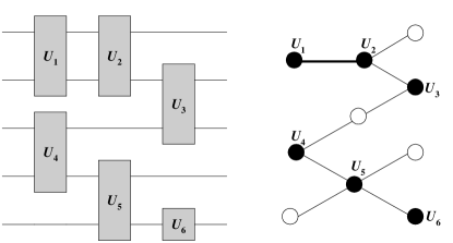
Figure 1: A simple quantum circuit and the corresponding interaction graph. The solid vertices correspond to nontrivial quantum gates, the empty vertices correspond to identity gates. Thick edges are those that resulted from the collapsing operation on the intermediate multigraph.

The vertices of $\Gamma_{C}$ can now be thought of as the potential locations of errors, so that an error that occurs at some $v\in V_{C}$ can propagate to some or all of $v^{\prime}\in V_{C}$ for which $v\leftrightarrow v^{\prime}$. Assuming that there are no correlations between errors in distinct gates, either in space or in time (which is the focus of this paper), we lose no generality if we suppose that $\Gamma_{C}$ is connected, i.e., there exists a path between any two $v,v^{\prime}\in\Gamma_{C}$. (Otherwise we could represent $\Gamma_{C}$ as a union of maximal connected subgraphs, $\Gamma_{C}=\Gamma^{1}_{C}\cup\ldots\cup\Gamma^{L}_{C}$, so that if an error occurs in some $\Gamma^{i}_{C}$, $1\leq i\leq L$, it will not propagate to any $\Gamma^{j}_{C}$ with $j\neq i$.) Another important feature of the graph $\Gamma_{C}$ is that, even if it corresponds to an “infinitely large” quantum circuit, its vertices have bounded coordination number, i.e.,

$$\max_{v\in V_{C}}\#\left(\{v^{\prime}\in V_{C}\,|\,v\leftrightarrow v^{\prime}\}\right)<\infty,$$

where $\#(S)$ denotes cardinality of the set $S$. Basically, this is a consequence of the fact that all quantum gates in any universal set act on finitely many qubits.

As for the error model, we will content ourselves with the simplest scenario. Namely, some $\eta\in(0,1)$ is picked, and we assume that each gate (including identity gates) undergoes an error with probability $\eta$ and functions correctly with probability $1-\eta$. This is known as the assumption of local stochastic faults ab . Quantum operations that describe errors within this model have the form ${\mathbf{T}}(\rho)=(1-\eta)\rho+\eta{\mathbf{T}}^{\prime}(\rho)$, where ${\mathbf{T}}^{\prime}$ is a quantum operation whose Kraus operators act nontrivially only on the qubits participating in a particular quantum gate.

Under this simple model, the occurrence of errors in space and time is described naturally by a process known as Bernoulli site percolation hug on the interaction graph $\Gamma_{C}$. Namely, each vertex $v\in V_{C}$ is occupied with probability $\eta$ and vacant with probability $1-\eta$, independently of all other vertices, so that the occupied vertices correspond to the locations of errors. Configurations of occupied and vacant vertices are given by elements of the sample space $\Omega_{C}:=\{0,1\}^{V_{C}}$, where $0$ ($1$) indicates a vacant (occupied) vertex; the probability of an event $F\subseteq\Omega_{C}$ will be denoted by ${\mathbb{P}}_{\eta}(F)$ [note the explicit parametrization of all probabilities by the vertex occupation density $\eta$]. An edge $v\leftrightarrow v^{\prime}$ is called open if both $v$ and $v^{\prime}$ are occupied, and closed otherwise. A set $K\subset V_{C}$ is called a cluster (of connected occupied vertices) if all edges $v\leftrightarrow v^{\prime}$ with $v,v^{\prime}\in K$ are open, and all edges $v\leftrightarrow v^{\prime}$ with $v\in K$, $v^{\prime}\in V_{C}\backslash K$ are closed. Among other things, percolation theory is concerned with statistical properties of clusters as the occupation density $\eta$ is varied.

By construction, the interaction graph $\Gamma_{C}$ and the corresponding site percolation process have the following properties: (i) $\Gamma_{C}$ is statistically homogeneous, i.e., the probability that a vertex is occupied does not depend on its location in $\Gamma_{C}$, and (ii) the number of vertices that can be reached from a given vertex by paths of length $n$ or less is $O(2^{cn})$ for some $c<1$. Then it follows from general arguments of percolation theory hug that: (1) there exists a number $\eta_{*}>0$ (the percolation threshold note1 ) such that, in the limit of an infinite number of vertices, the probability of a given vertex belonging to an infinite cluster of occupied vertices is zero for $\eta<\eta_{*}$, and strictly greater than zero for $\eta>\eta_{*}$; and (2) for $\eta<\eta_{*}$, the expected cluster size is finite.

We now show that an estimate of the threshold error rate may be derived by means of a renormalization argument common in percolation theory (see, e.g., Chap. 4 of hug for details). The basic idea is the following: an (infinite) graph $\Gamma$ is “coarse-grained” by means of a rule that replaces suitably defined groups of vertices of $\Gamma$ with single vertices, prescribes how these new vertices are to be connected by edges, and defines a new occupation probability $\eta^{\prime}$ on the resulting graph $\Gamma^{\prime}$. Typically, if we start with a subcritical ($\eta<\eta_{*}$) percolation proces on $\Gamma$, the net result of iterating the renormalization process will be to push the system away from $\eta_{*}$ towards the “trivial” behavior ($\eta\rightarrow 0$).

Given a quantum circuit $C_{0}$, consider the single-layer encoding $C_{1}=M(C_{0})$ and the accompanying quantum computation code. Let $A$ be the maximum number of locations involved in a single procedure in $C_{1}$, $d$ the maximum number of errors corrected by the code, $s$ the spread of the code, and $k=\lfloor d/s\rfloor$. Fix a particular procedure in $C_{1}$. Then, if more than $d$ qubits are in error at the end of this procedure, the recovery stage of the subsequent procedure will fail. This will happen precisely when at least $k+1$ errors occur during the procedure. Denote this event by $E$. Using subadditivity of the probability measure ${\mathbb{P}}_{\eta}(\cdot)$ and properties of the binomial coefficients, we readily obtain the bound

$${\mathbb{P}}_{\eta}(E)\leq\sum^{A}_{\ell=k+1}{A\choose\ell}\eta^{\ell}(1-\eta)^{A-\ell}\leq 2^{A}\eta^{k+1}.$$

Then, for any $\eta$ satisfying the threshold condition $\eta<\eta_{c}\equiv 2^{-A/k}$, we have ${\mathbb{P}}_{\eta}(E)<\eta$, i.e., the probability of $k$ or more errors during a procedure is smaller than the probability of a single error.

The influence of concatenation on the effective error rate can now be understood as follows. Consider the interaction graph $\Gamma_{C_{1}}$ associated with the circuit $C_{1}=M(C_{0})$. We “renormalize” it by replacing the vertices corresponding to each procedure in $C_{1}$ with a single vertex, and then by drawing edges appropriately. From considerations of self-similarity we can expect that the resulting renormalized graph $R(\Gamma_{C_{1}})$ is isomorphic to $\Gamma_{C_{0}}$. We then say that a vertex $v$ of $R(\Gamma_{C_{1}})$ is occupied if at least $k+1$ errors occur in the corresponding procedure in $C_{1}$, and vacant otherwise. We will denote the occupation density in $R(\Gamma_{C_{1}})$ by $R(\eta)$; it is related to the “original” occupation probability $\eta$ through $R(\eta)={\mathbb{P}}_{\eta}(E)$.

When $\eta<\eta_{c}$, $R(\eta)\leq 2^{A}\eta^{k+1}<\eta$. That is, iteration of the renormalization process will keep reducing the occupation probability further, as $R^{r+1}(\eta)<R^{r}(\eta)<\ldots<\eta$. Better upper bounds on the renormalized occupation densities can be easily computed by solving the recurrence $R^{r+1}(\eta)\leq 2^{A}[R^{r}(\eta)]^{k+1}$ with the initial condition $R^{0}(\eta)=\eta$, which yields

$$R^{r}(\eta) \leq 2^{A[1+(k+1)+\ldots+(k+1)^{r-1}]}\eta^{(k+1)^{r}}$$

$$= 2^{A[(k+1)^{r}-1]/k}\eta^{(k+1)^{r}}$$

$$= 2^{-A/k}\left[2^{A/k}\eta\right]^{(k+1)^{r}}.$$

Note that the occurrence of errors on the coarse-grained interaction graph is also modeled by a site percolation process because the errors in any given procedure are assumed to occur independently of the errors in all other procedures, and our renormalization transformation has been defined only in terms of the restriction of global error configurations to individual procedures. After $r$ levels of concatenation, the effective error rate is exactly the site occupation probability on $R^{r}(\Gamma_{C_{0}})$, and is bounded from above by $c^{-1}_{1}(c_{1}\eta)^{(1+c_{2})^{r}}$, where $c_{1},c_{2}$ are constants related to the particular quantum computation code used. The threshold condition on the error rate is therefore that $\eta<c^{-1}_{1}$.

The necessary number of concatenation levels can now be determined in the usual way preskill ; ab : if the unencoded circuit $C_{0}$ has $N$ gates, then the encoded circuit $C_{r}$ will have $N$ $r$-procedures, so that if we want the net computation error to be less than some $\epsilon>0$, the effective error rate must be at most $\epsilon/N$. This is guaranteed whenever $R^{r}(\eta)<\epsilon/N$, which yields $r=\operatorname{polylog}(N/\epsilon)$ note2 . That is, the complexity of the fault-tolerant quantum circuit will be larger than that of the unencoded circuit by a polylogarithmic factor.

The above estimate of the threshold is quite crude. The exact value of $\eta_{c}$ can be determined by finding nontrivial fixed points of the renormalization transformation $\eta\mapsto R(\eta)$ (note that the trivial values $\eta=0,1$ are also fixed points of $R$). It is not hard to see that the graph of $R$ has the “S-shape” shown in Fig. 2. The exact value $\eta_{c}$ of the threshold error rate is precisely the nontrivial fixed point of $R$. One can also use the “staircase construction” pictured there to see how the effective error rate goes down with the number of concatenation levels.

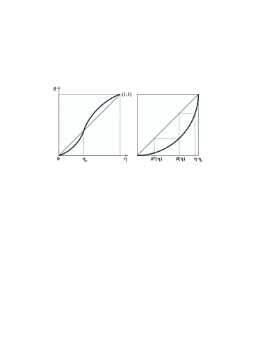
Figure 2: Left: the “S-shaped” curve of the renormalization transformation $R$. Right: the portion of the curve for $0\leq\eta\leq\eta_{c}$ and the “staircase construction” used to illustrate how the effective error rate is reduced under iteration of $R$.

Further information on the renormalized error rate $R(\eta)$ can be obtained by means of general arguments of percolation theory. To this end let us observe the following properties of the event $E$: (i) its occurrence depends on the status (i.e., occupied or vacant) of a finite number $\alpha$ of vertices, and (ii) it is an increasing event, i.e., stable under addition of more occupied vertices. Then the following differential inequality holds for $0<\eta<1$ ms ; ccfs :

$$\frac{R(\eta)\left(1-R(\eta)\right)}{\eta(1-\eta)}\leq R^{\prime}(\eta)\leq\sqrt{\frac{\alpha}{\eta(1-\eta)}},$$ (1)

where the prime denotes differentiation with respect to $\eta$. It follows easily from the first inequality in (1) that $\lambda\equiv R^{\prime}(\eta_{c})\geq 1$; in fact, a more careful analysis shows that $\lambda>1$ gri . From the second inequality in (1) we get the following relation holds between $\lambda$, $\alpha$, and $\eta_{c}$:

$$\lambda\leq\sqrt{\frac{\alpha}{\eta_{c}(1-\eta_{c})}}.$$ (2)

Consider now a quantum computer operating in the subthreshold regime, but very close to the threshold, i.e., $\eta_{c}-\delta<\eta<\eta_{c}$ for some small $\delta>0$. The minimum number of concatenation levels necessary to bring the effective error rate down to some suitable small value $\epsilon$ (where we can assume that $\delta\ll\eta_{c}-\epsilon$) is controlled by $\lambda$ (see the staircase construction in Fig. 2). Linearizing $R$ around $\eta_{c}$ as $R(\eta)=\eta_{c}+\lambda(\eta-\eta_{c})+o(|\eta-\eta_{c}|)$ and iterating this process $r$ times, we see that we need to pick $r$ such that $\eta_{c}-\epsilon<\lambda^{r}\delta$, i.e., it suffices to take

$$r\simeq\left\lfloor\frac{\log[(\eta_{c}-\epsilon)/\delta]}{\log\lambda}\right\rfloor.$$ (3)

Solving (3) for $\lambda$, substituting into (2), and using the fact that $(\eta_{c}-\epsilon)^{2/r}\geq(\eta_{c}-\epsilon)^{2}$ for $r\geq 1$ and $0<\epsilon<\eta_{c}<1$, we get

$$\eta_{c}(1-\eta_{c})(\eta_{c}-\epsilon)^{2}\leq\alpha\delta^{2/r}.$$ (4)

This inequality can be regarded as a threshold-overhead tradeoff inequality: it shows that fault-tolerant quantum circuits with low concatenation overhead must have correspondingly small threshold error rates, and conversely that fault-tolerant quantum circuits with large threshold rates have the distinct disadvantage of requiring high concatenation overhead.

Let us close with a few remarks. First of all, we have so far paid no attention to the percolation threshold $\eta_{*}$ on $\Gamma_{C}$ and how it compares to $\eta_{c}$. We expect that $\eta_{c}\ll\eta_{*}$ on the grounds that the (connected) clusters of malfunctioning gates should be highly dilute in order for error correction to succeed. Also, the methods used in this paper are applicable to noisy classical computers as well. (This is, ultimately, not very surprising in light of the fact that the local stochastic error model is, essentially, classical in spirit.) It would be interesting and useful to extend the methods used in this paper (and percolation-theoretic methods in general) to less idealized models of noise in quantum computers. A promising step in this direction would be an application of percolation techniques to problems involving graph-theoretic models of multiparticle entanglement qgraphs1 and quantum computation qgraphs2 .

References

- (1) A.Yu. Kitaev, in Quantum Communication, Computing, and Measurement, ed. by O. Hirota and C.M. Caves (Plenum Press, New York, 1997), pp. 181–188.
- (2) E. Knill, R. Laflamme, and W. Zurek, Proc. R. Soc. London, Ser. A 454, 365 (1998).
- (3) J. Preskill, Proc. R. Soc. London, Ser. A 454, 385 (1998).
- (4) D. Aharonov and M. Ben-Or, arXiv e-print quant-ph/9906129 (1999).
- (5) P. Gács, J. Comp. Sys. Sci. 32, 15 (1986).
- (6) B.D. Hughes, Random Walks and Random Environments, vol. 2 (Clarendon Press, Oxford, 1996).
- (7) E. Knill and R. Laflamme, Phys. Rev. A55, 900 (1997).
- (8) A. Barenco et al., Phys. Rev. A52, (1995).
- (9) We are deviating from the common practice in percolation theory of using the subscript ‘’ to denote the percolation threshold because it is common practice in the theory of fault-tolerant quantum computation to use this subscript for the threshold error rate.
- (10) The notation is used whenever we can find positive constants , such that .
- (11) E.F. Moore and C.E. Shannon, J. Franklin Inst. 262, 191 (1956); 262, 281 (1956).
- (12) J.T. Chayes, L. Chayes, D.S. Fisher, and T. Spencer, Phys. Rev. Lett. 57, 2999 (1986).
- (13) G. Grimmett, Percolation, 2nd ed. (Springer-Verlag, Berlin, 1999).
- (14) M. Plesch and V. Bužek, Quant. Inf. Comp. 2, 530 (2002); M. Hein, J. Eisert, and H.J. Briegel, arXiv e-print quant-ph/0307130 (2003).
- (15) R. Raussendorf and H.J. Briegel, Quant. Inf. Comp. 2, 443 (2002); D. Schlingemann, arXiv e-print quant-ph/0305170 (2003).