Measurement and Information Extraction in Complex
Dynamics Quantum Computation

Measurement and Information Extraction in Complex Dynamics Quantum Computation

Quantum Information processing has several different applications: some of them can be performed controlling only few qubits simultaneously (e.g. quantum teleportation or quantum cryptography) steane . Usually, the transmission of large amount of information is performed repeating several times the scheme implemented for few qubits. However, to exploit the advantages of quantum computation, the simultaneous control of many qubits is unavoidable chuang . This situation increases the experimental difficulties of quantum computing: maintaining quantum coherence in a large quantum system is a difficult task. Indeed a quantum computer is a many-body complex system and decoherence, due to the interaction with the external world, will eventually corrupt any quantum computation. Moreover, internal static imperfections can lead to quantum chaos in the quantum register thus destroying computer operability GS . Indeed, as it has been shown in term , a critical imperfection strength exists above which the quantum register thermalizes and quantum computation becomes impossible. We showed such effects on a quantum computer performing an efficient algorithm to simulate complex quantum dynamics simone1 ; simone2 .

In this paper, we address a different and very general problem related to the extraction of the information. Indeed, the information is encoded in the wave function, and apart from very particular situations, it is hard to find a way to address and extract the useful information. Commonly, when trying to extract information, the efficiency of quantum information processing is lost. This is one of the main problem to solve while looking for new quantum algorithms. However, in some cases, these difficulties can be bypassed, as in Shor, Grover and other well known quantum algorithms ekert .

The problem of extracting information is particularly difficult in one of the most general quantum computing applications: the simulation of many-body complex quantum systems. Indeed, the results of such simulations is, typically, the quantum state: the wave function as a whole. The problems is that, in order to measure all $N$ wave function coefficients (coded in $n_{q}=log_{2}(N)$ qubits) by means of a projective measurement, one must repeat the calculus $O(N)$ times. This destroys the efficiency of any quantum algorithm even in the case in which such algorithm can compute the wave function with an exponential gain in the number $n_{q}$ of elementary gates.

However, as it is the case for other quantum algorithms, there are some questions that can be answered in an efficient way. Here we present an interesting example where important information can be extracted efficiently by means of quantum simulations. We show how this methods work on a dynamical model, the so-called Sawtooth Map simone1 . This map is characterized by very different dynamical regimes: from near integrable to fully developed chaos; it also exhibits quantum dynamical localization percival ; prosen . We show how to extract efficiently the localization length and the mean square deviation. The results obtained here for the sawtooth map can shed some light for the study of different quantum systems. Indeed, as it is well known, any classical simulation of a quantum system will pretty soon be limited by lack of computational resources. In our work we show how some questions can be answered efficiently by means of a quantum computer, thus allowing the investigation of some general properties beyond the reach of classical supercomputers.

This paper is organized as follows: in section I we introduce our model: the Sawtooth Map. In Section II the quantum algorithm to compute the quantum motion is presented in detail. In Section III we review the exponentially efficient calculation of dynamical localization length. Finally, in Section IV, we discuss the additional information that can be extracted. Our conclusions are summarized in Section V.

1 Sawtooth Map

The classical sawtooth map is given by

$$\overline{n}={n}+k(\theta-\pi),\quad\overline{\theta}=\theta+T\overline{n},$$ (1)

where $(n,\theta)$ are conjugated action-angle variables ($0\leq\theta<2\pi$), and the bars denote the variables after one map iteration. Introducing the rescaled variable $p=Tn$, one can see that the classical dynamics depends only on the single parameter $K=kT$. The map (1) can be studied on the cylinder ($p\in(-\infty,+\infty)$), which can also be closed to form a torus of length $2\pi L$, where $L$ is an integer. For any $K>0$, the motion is completely chaotic and one has normal diffusion: $<(\Delta p)^{2}>\approx D(K)t$, where $t$ is the discrete time measured in units of map iterations and the average $<\cdots>$ is performed over an ensemble of particles with initial momentum $p_{0}$ and random phases $0\leq\theta<2\pi$. It is possible to distinguish two different dynamical regimes percival : for $K>1$, the diffusion coefficient is well approximated by the random phase approximation, $D(K)\approx(\pi^{2}/3)K^{2}$, while for $0<K<1$ diffusion is slowed down, $D(K)\approx 3.3K^{5/2}$, due to the sticking of trajectories close to broken tori (cantori). For $-4<K<0$ the motion is stable, the phase space has a complex structure of elliptic islands down to smaller and smaller scales, and we observed anomalous diffusion, $<(\Delta p)^{2}>\propto t^{\alpha}$, (for example, $\alpha=0.57$ when $K=-0.1$). Inside each island the motion can be approximated by an harmonic oscillator, as can be easily view by the fixed points stability analysis. In Fig. 1 we show a typical phase space of the classical sawtooth map for $K=-0.3$.

The quantum evolution on one map iteration is described by a unitary operator $\hat{U}$ acting on the wave function $\psi$:

$$\overline{\psi}=\hat{U}\psi=e^{-iT\hat{n}^{2}/2}e^{ik(\hat{\theta}-\pi)^{2}/2}\psi,$$ (2)

where $\hat{n}=-i\partial/\partial\theta$ (we set $\hbar=1$). Equation (2) is obtained by integrating over one period $T$ the Schrödinger equation. As we set $\hbar=1$, one has $[\theta,p]=T[\theta,n]=iT$ giving $\hbar_{eff}=T$. Thus, the classical limit corresponds to $T\to 0$, $k\to\infty$, and $K=kT=\hbox{const}$. In this quantum model one can observe important physical phenomena like dynamical localization prosen ; fausto . Indeed, similarly to other models of quantum chaos krot , the quantum interference in the sawtooth map leads to suppression of classical chaotic diffusion after a break time

$$t^{\star}\approx D_{n}\approx(\pi^{2}/3)k^{2},$$ (3)

where $D_{n}$ is the classical diffusion coefficient, measured in number of levels ($<(\Delta n)^{2}>\approx D_{n}t$). For $t>t^{\star}$ only $\Delta n\sim D_{n}$ levels are populated and the localization length $\ell\sim\Delta n$ for the average probability distribution is approximately equal ds1987 :

$$\ell\approx D_{n}$$ (4)

Thus the quantum localization can be detected if $\ell$ is smaller than the system size $N$.

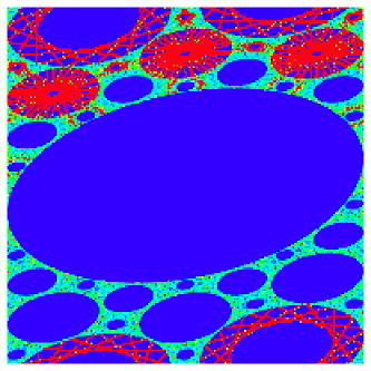
Figure 1: The phase space of the classical Sawtooth map for $K=-0.3$. The phase space density plot is obtained form an ensemble of $10^{4}$ trajectories with initial $n_{0}$ and random phases outside the main island (big blue central area). $-\pi\leq p<\pi$ (vertical axis), $0\leq\theta<2\pi$ (horizontal axis). The probability density is proportional to colors: blue for zero, red for maximal probability.

In Section 3, we study the map (2) in the deep quantum regime of dynamical localization. For this purpose, we keep $k,K$ constant. Thus the effective Planck constant is fixed and the number of cells $L$ grows exponentially with the number of qubits ($L=TN/2\pi$). In this case, one studies the quantum sawtooth map on the cylinder ($n\in(-\infty,+\infty)$), which is cut-off to a finite number of cells due to the finite quantum (or classical) computer memory.

Notice that keeping $K$ and $L$ constant while increasing the number of qubits, allows the study of the quantum to classical transition. Moreover, in the stable case, $-4<K<0$, one can study the wave function evolution inside and outside the islands. In the first case, the motion follows the classical periodic motion with a given characteristic frequency $\omega$, while outside the classical anomalous diffusion can be suppressed by quantum effects.

We stress again that, since in a quantum computer the memory capabilities grow exponentially with the number of qubits, already with less than 40 qubits one could make simulations inaccessible for today’s supercomputers.

2 Quantum algorithm

The quantum algorithm introduced in simone1 simulates efficiently the quantum dynamics (2) using a register of $n_{q}$ qubits. It is based on the forward/backward quantum Fourier transform qft between the $\theta$ and $n$ representations and has some elements of the quantum algorithm for kicked rotator GS1 . Such an approach is rather convenient since the Floquet operator $\hat{U}$ is the product of two operators $\hat{U}_{k}=e^{ik(\hat{\theta}-\pi)^{2}/2}$ and $\hat{U}_{T}=e^{-iT\hat{n}^{2}/2}$: the first one is diagonal in the $\hat{\theta}$ representation, the latter in the $\hat{n}$ representation. Moreover both operators can be decomposed in a sequence of controlled phase shifts without using any temporary storing register.

The quantum algorithm for one map iteration requires the following steps:
I. The unitary operator $\hat{U}_{k}$ is decomposed in $n_{q}^{2}$ two-qubit gates

$$e^{\imath k(\theta-\pi)^{2}/2}=\prod_{i,j}e^{\imath 2\pi^{2}k(\alpha_{i}2^{-i}-\frac{1}{2n_{q}})(\alpha_{j}2^{-j}-\frac{1}{2n_{q}})},$$ (5)

where $\theta=2\pi\sum\alpha_{i}2^{-i}$, with $\alpha_{i}\in\{0,1\}$. Each two-qubit gate can be written in the $\{|00\rangle,|01\rangle,|10\rangle,|11\rangle\}$ basis as $\exp(ik\pi^{2}D)$, where D is a diagonal matrix with elements

$$\{\frac{1}{2n_{q}^{2}},-\frac{1}{n_{q}}\left(\frac{1}{2^{j}}-\frac{1}{2n_{q}}\right),-\frac{1}{n_{q}}\left(\frac{1}{2^{i}}-\frac{1}{2n_{q}}\right),$$

$$2\left(\frac{1}{2^{i}}-\frac{1}{2n_{q}}\right)\left(\frac{1}{2^{j}}-\frac{1}{2n_{q}}\right)\}.$$ (6)

II. The change from the $\theta$ to the $n$ representation is obtained by means of the quantum Fourier transform, which requires $n_{q}$ Hadamard gates and $n_{q}(n_{q}-1)/2$ controlled-phase shift gates qft .
III. In the new representation the operator $\hat{U}_{T}$ has essentially the same form as $\hat{U}_{k}$ in step I and therefore it can be decomposed in $n_{q}^{2}$ gates similarly to equation (5).
IV. We go back to the initial $\theta$ representation via inverse quantum Fourier transform.
On the whole the algorithm requires $3n_{q}^{2}+n_{q}$ gates per map iteration. Therefore it is exponentially efficient with respect to any known classical algorithm. Indeed the most efficient way to simulate the quantum dynamics (2) on a classical computer is based on forward/backward fast Fourier transform and requires $O(n_{q}2^{n_{q}})$ operations. We stress that this quantum algorithm does not need any extra work space qubit. This is due to the fact that for the quantum sawtooth map the kick operator $\hat{U}_{k}$ has the same quadratic form as the free rotation operator $\hat{U}_{T}$.

Figure 2: Probability distribution over the momentum basis with $n_{q}=6$ qubits for $k=\sqrt{3}$ and initial momentum $n_{0}=0$; the numerical data are averaged in the intervals $10\leq t\leq 20$ (full curve) and $290\leq t\leq 300$ (dashed curve). The straight line fit, $W_{n}\propto\exp(-2|n|/\ell)$, gives the localization length $\ell\approx 12$.

3 Simulation of dynamical localization

In Fig. 2, we show that, using our quantum algorithm, exponential localization can be clearly seen already with $n_{q}=6$ qubits. After the break time $t^{\star}$, the probability distribution over the momentum eigenbasis decays exponentially,

$$W_{n}=|\hat{\psi}(n)|^{2}\approx\frac{1}{\ell}\exp\left(-\frac{2|n-n_{0}|}{\ell}\right),$$ (7)

with $n_{0}=0$ the initial momentum value. Here the localization length is $\ell\approx 12$, and classical diffusion is suppressed after a break time $t^{\star}\approx\ell$, in agreement with the estimates (3)-(4). This requires a number $N_{g}\approx 3n_{q}^{2}\ell\sim 10^{3}$ of one- or two-qubit quantum gates. The full curve of Fig. 2 shows that an exponentially localized distribution indeed appears at $t\approx t^{\star}$. Such distribution is frozen in time, apart from quantum fluctuations, which we partially smooth out by averaging over a few map steps. The localization can be seen by the comparison of the probability distributions taken immediately after $t^{\star}$ (full curve in Fig. 2) and at a much larger time $t=300\approx 25t^{\star}$ (dashed curve in the same figure).

We now discuss how it would be possible to extract information (the value of the localization length) from a quantum computer simulating the above described dynamics. The localization length can be measured by running the algorithm several times up to a time $t>t^{\star}$. Each run is followed by a standard projective measurement on the computational (momentum) basis. The outcomes of the measurements can be stored in histogram bins of width $\delta n\propto\ell$, and then the localization length can be extracted from a fit of the exponential decay of this coarse-grained distribution over the momentum basis. In this way the localization length can be obtained with accuracy $\nu$ after the order of $1/\nu^{2}$ computer runs. It is important to note that it is sufficient to perform a coarse grained measurement to generate a coarse grained distribution. This means that it will be sufficient to measure the most significant qubits, and ignore those that would give a measurement accuracy below the coarse graining $\delta n$. Thus, the number of runs and measurements is independent of $\ell$. However, it is necessary to make about $t^{\star}\sim\ell$ map iterations to obtain the localized distribution (see Eqs. (3,4)). This is true both for the present quantum algorithm and for classical computation. This implies that a classical computer needs $O(\ell^{2}\log\ell)$ operations to extract the localization length, while a quantum computer would require $O(\ell(\log\ell)^{2})$ elementary gates (classically one can use a basis size $N\sim\ell$ to detect localization). In this sense, for $\ell\sim N=2^{n_{q}}$ the quantum computer gives a square root speed up if both classical and quantum computers perform $O(N)$ map iterations. However, for a fixed number of iterations $t$ the quantum computation gives an exponential gain. For $\ell\ll N$ such a gain can be very important for more complex physical models, in order to check if the system is truly localized harper .

4 Efficient Measurements

We now discuss how some other important system’s characteristic quantity can be extracted efficiently by means of a quantum simulation. We would like to stress that our procedure can be applied to any quantum system with a similar dynamics simulated on a quantum computer.

As for the localization length, also the mean squared moment can be efficiently extracted with a given precision. Indeed, for a fixed number of iterations $t$ the quantum computation gives an exponential gain since one should compare $O(t(\log N)^{2})$ gates (quantum computation) with $O(tN\log N)$ gates (classical computation). Starting from the wave function, by repeating $\nu$ projective measurements, it is possible to get the mean squared moment and therefore the diffusion coefficient $D_{n}\approx<(\Delta n(t))^{2}>/t$. This is an important characteristic which determines the transport properties of the system.

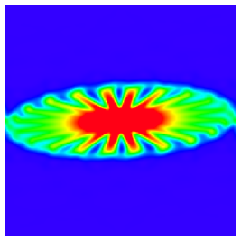
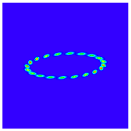
Figure 3: Husimi function husimi of the Sawtooth Map for $K=-0.1,T=2\pi/N,s=\Delta p\Delta\theta=1$, $-\pi\leq p<\pi,0\leq\theta<2\pi$. Probability is proportional to colors: blue for zero, red for maximal probability. Initial conditions: a momentum eigenstate (left), a coherent state (right). The Husimi functions are averaged over twenty map steps.

In a similar way one can compute $<(\Delta n(t))^{2}>$ in the classical limit which is obtained by keeping $K,L$ constant and increasing $N$. Correspondingly, the number of qubits increases and therefore one can explore smaller and smaller scales of the phase space, that is, of the wave function. This can be fundamental in complex systems with fractal or self-similar structures in order to determine the nature of the diffusion in the system, e.g. discriminating from anomalous or brownian diffusion. Notice that classically, investigating smaller scales needs exponential efforts. On the contrary, only a polynomial increasing of resources is needed when performing a quantum simulation.

Finally we would like to mention another important feature which can be efficiently extracted. Indeed if, as in our model for $-4<K<0$, an island is present in the system phase space, one can extract the island characteristic frequency $\omega$. Two typical procedures are possible: the first one can be applied if the island size is comparable with the system size (at least in momentum or phase representation). This is the case of the principal island of our model (see Fig. 3, left). Indeed, starting from a momentum eigenstate inside the resonance, the wave function will expand and squeeze periodically. Thus, computing the squared moment deviation at different times one can recover $\omega$. In the case that the island is small compared to system size, one can start with a localized wave function inside it, e.g. a coherent state. Although coherent states are more difficult to prepare with respect to momentum or phase eigenfunctions, in the case of fixed $K,k$, the number of operations needed to prepare such states is $N$-independent. Under the dynamical evolution a coherent state will periodically return back to its initial position (Fig. 3, right). As before, measuring the wave packet center of mass at different times, it is possible to estimate the frequency $\omega$.

5 Conclusions

We discuss the problem of information extraction in quantum simulation of complex systems. We present some examples of how quantum computation can be useful to efficiently extract important information as localization length, mean square deviation and system’s characteristic frequency. Notice that, in general, extracting the information embedded in the wave function is not an efficient process, however we show that in some cases quantum simulations can be exponentially efficient with respect to classical ones. We study in particular the quantum sawtooth map algorithm which can be an optimum test for such simulations and requires only a number of qubits less than ten.

Finally, we stress that the procedure discussed here is not restricted to the sawtooth map but can be applied to more general quantum system.

This research was supported in part by the EC RTN contract HPRN-CT-2000-0156, the NSA and ARDA under ARO contracts No. DAAD19-02-1-0086, the project EDIQIP of the IST-FET programme of the EC and the PRIN-2002 “Fault tolerance, control and stability in quantum information processing”.

References

- (1) A.Steane, Rep. Prog. Phys. 61, 117 (1998).
- (2) See, e.g., M.A. Nielsen and I.L. Chuang, Quantum Computation and Quantum Information (Cambridge University Press, Cambridge, 2000).
- (3) B. Georgeot and D.L. Shepelyansky, Phys. Rev. E 62, 3504 (2000); 62, 6366 (2000)
- (4) G. Benenti, G. Casati, D. L. Shepelyansky, Eur. Phys. J. D 17, 265 (2001).
- (5) G. Benenti, G. Casati, S. Montangero, and D.L. Shepelyansky, Phys. Rev. Lett. 87, 227901 (2001).
- (6) G. Benenti, G. Casati, S. Montangero, and D.L. Shepelyansky, Eur. Phys. J. D 20, 293 (2002); Eur. Phys. J. D 22, 285 (2003).
- (7) A. Ekert, P. Hayden, H. Inamori Les Houches Summer School on ”Coherent Matter Waves”, (1999).
- (8) I. Dana, N.W. Murray, and I.C. Percival, Phys. Rev. Lett. 62, 233 (1989); Q. Chen, I. Dana, J.D. Meiss, N.W. Murray, and I.C. Percival, Physica D 46, 217 (1990).
- (9) G. Casati and T. Prosen, Phys. Rev. E 59, R2516 (1999).
- (10) F. Borgonovi, G. Casati, and B. Li, Phys. Rev. Lett. 77, 4744 (1996); F. Borgonovi, Phys. Rev. Lett. 80, 4653 (1998); G. Casati and T. Prosen, Phys. Rev. E 59, R2516 (1999).
- (11) T. Geisel, G. Radons, and J. Rubner, Phys. Rev. Lett. 57, 2883 (1986).
- (12) R.S. MacKay and J.D. Meiss, Phys. Rev. A 37, 4702 (1988).
- (13) R.E. Prange, R. Narevich, and O. Zaitsev, Phys. Rev. E 59, 1694 (1999).
- (14) B. Georgeot and D.L. Shepelyansky, Phys. Rev. Lett. 86, 2890 (2001).
- (15) D.L. Shepelyansky, Physica D 28, 103 (1987).
- (16) See, e.g., A. Ekert and R. Jozsa, Rev. Mod. Phys. 68, 733 (1996).
- (17) B. Georgeot , and D.L. Shepelyansky, Phys. Rev. Lett. 86, 2890 (2001).
- (18) T. Prosen, I.I. Satija, and N. Shah, Phys. Rev. Lett. 87, 066601 (2001), and references therein.
- (19) The computation of Husimi functions is described in S.-J. Chang and K.-J. Shi, Phys. Rev. A 34, 7 (1986).