On the Quantum Phase Operator for Coherent States

Abstract

In papers by Lynch [Phys. Rev. A41, 2841 (1990)] and Gerry and Urbanski [Phys. Rev. A42, 662 (1990)] it has been argued that the phase-fluctuation laser experiments of Gerhardt, Büchler and Lifkin [Phys. Lett. 49A, 119 (1974)] are in good agreement with the variance of the Pegg-Barnett phase operator for a coherent state, even for a small number of photons. We argue that this is not conclusive. In fact, we show that the variance of the phase in fact depends on the relative phase between the phase of the coherent state and the off-set phase $\phi_{0}$ of the Pegg-Barnett phase operator. This off-set phase is replaced with the phase of a reference beam in an actual experiment and we show that several choices of such a relative phase can be fitted to the experimental data. We also discuss the Noh, Fougères and Mandel [Phys. Rev. A46, 2840 (1992)] relative phase experiment in terms of the Pegg-Barnett phase taking post-selection conditions into account.

PACS Ref:42.50-p;42.50.Gy;42.50.Xa

I INTRODUCTION

The notion of a quantum phase and a corresponding quantum phase operator plays an important role in various considerations in e.g. modern quantum optics (for a general discussion see e.g. Refs.Carr68 ; barnett97 ; SB93 ). Recently it has been argued by R. Lynch Lynch90 and C. C. Gerry and K. E. Urbanski Gerry90 that the theoretical values of the variance of the Pegg-Barnett (PB) phase operator Pegg89 evaluated for a coherent state are in good agreement with the phase-fluctuation measurements of Gerhardt, Büchler and Lifkin (GBL) Gerhardt74 for two interfering laser beams. In the literature one often finds reiterations of this statement (see e.g. Ref.Orzag2000 ). For the purpose of analyzing the experimental data in terms of the PB phase operator one makes the assumption that the laser light can be described in terms of a conventional coherent state (see e.g. Ref.Klauder&Skagerstam&85 ). It has, however, been questioned to what extent this assumption is correct Moelmer1997 based on the fact that conventional theories of a laser naturally leads to a mixed rather than a pure quantum state (see e.g. Ref.Scully&Zubairy ). Relative to a reference laser beam the quantum state of the laser can nevertheless be assumed to be a coherent state Enk . We notice that the arguments of Ref.Moelmer1997 has been questioned Gea1998 and that in some laser models there are indeed mechanisms which may provide for quantum states with precise values of both the amplitude and the phase. Recent experimental developments have also actually lead to a precise measurement of the amplitude and phase of short laser pulses Walther2001 .

In the present paper it is assumed that a coherent state is a convenient description of the quantum state of the laser in agreement with our argumentation above. Even with the use of coherent states we will claim that a clarification is required concerning the comparison between the PB quantum phase theory and experimental data. We will argue that the phase is naturally given relative to the PB off-set phase $\phi_{0}$ and that the variance of the relative phase $\hat{\phi}-\phi_{0}$ therefore is dependent on the relative phase between the phase $\xi$ of the coherent state and the off-set phase $\phi_{0}$. In an actual experiment one measures the phase relative to a reference beam and the off-set value $\phi_{0}$ will then effectively be replaced by the phase of the reference beam. In the course of our calculations and in comparing with experimental data, we will verify that in some situations the actual phase in the definition of the coherent state used is actually irrelevant. In the course of our considerations below, we will compare the PB approach to the notion of a quantum phase with other defintions and point out situations where they are in agreement or disagreement with actual experimental observations. The paper is organized as follows. In Section II we briefly review the PB quantum phase operator theory. Phase fluctuations in the PB theory and in the Susskind-Glogower (SG) theory Sussk64 ; Carr68 are discussed in Section III and various bounds on phase fluctuations are derived. Relative PB and SG phase operators are discussed in Section IV together with a comparison to the GBL experimental data Gerhardt74 . The PB theory and the Noh-Fougères-Mandel (NFM) Noh91 ; Noh92 ; Noh92_2 operational theory for a relative phase operator measurement are discussed in Section V and, finally, some concluding comments are given in Section VI.

II THE PB QUANTUM PHASE OPERATOR

We make use of a spectral resolution of the PB phase operator Pegg89 defined on a ($s+1$)-dimensional truncated Hilbert space of states, i.e.

$$\hat{\phi} =\sum_{m=0}^{s}\phi_{m}\lvert\phi_{m}\rangle\langle\phi_{m}\rvert$$ (1)

where

$$\phi_{m} =\phi_{0}+\frac{2\pi m}{s+1}\ \ \,;\ \ m=0,1,\ldots,s.$$ (2)

In Eq.(1) the normalized state $\lvert\phi_{m}\rangle$ can be expressed in terms of the number-operator eigenstates $\lvert n\rangle$, i.e.

$$\lvert\phi_{m}\rangle=\frac{1}{\sqrt{1+s}}\sum_{n=0}^{s}e^{in\phi_{m}}\lvert n\rangle~{}~{}.$$ (3)

As described by Pegg and Barnett Pegg89 , we do all the calculations of the physical quantities in this truncated space and take the limit $s\rightarrow\infty$ in the end. Care must be taken when performing the appropriate mathematical limit Lynch90 ; Troubles . Following these definitions, the expectation value of a function ${\cal O}$ of the relative phase operator $\hat{\phi}-\phi_{0}$ is given by

$$\langle{\cal O}\rangle\equiv\lim_{s\rightarrow\infty}\langle\psi\lvert{\cal O}(\hat{\phi}-\phi_{0})\rvert\psi\rangle =\int_{0}^{2\pi}d\phi\,{\cal O}(\phi)\,P(\phi)~{}~{},$$ (4)

where $\lvert\psi\rangle$ is a general pure quantum state in the form of a linear superposition of number-operator eigenstates $\lvert n\rangle$, i.e.

$$\lvert\psi\rangle =\sum_{n=0}^{\infty}\sqrt{{\cal P}_{n}}e^{i\xi(n)}\lvert n\rangle~{}~{},$$ (5)

with a normalized number-operator probability distribution ${\cal P}_{n}$. Here

$$P(\phi) =\frac{1}{2\pi}\left|\sum_{n=0}^{\infty}\sqrt{{\cal P}_{n}}\,e^{in(\phi+\phi_{0})-i\xi(n)}\right|^{2}$$ (6)

is a periodic probability distribution. The distribution $P(\phi)$ is the same as the one obtained from the SG phase operator theory Sussk64 , which has been argued on general grounds to be the case Shapiro91 . In the case of coherent-like states with $\xi(n)=n\xi+\xi_{0}$ but with arbitrary ${\cal P}_{n}$, the distribution $P(\phi)$ depends in general on the difference between the phase $\xi$ and the PB off-set value $\phi_{0}$, i.e. on $\delta\xi\equiv\xi-\phi_{0}$. For a coherent state $\lvert\psi\rangle=\lvert\alpha\rangle$, with $\alpha=|\alpha|\,e^{i\xi}$, the photon-number distribution is Poissonian, i.e. ${\cal P}_{n}=e^{-|\alpha|^{2}}|\alpha|^{2n}/n!$ . The mean value of the number of photons, ${\bar{n}}$, is then given by ${\bar{n}}=|\alpha|^{2}$. In what follows we will, unless otherwise specified, limit ourselves to the use of coherent states but our considerations can be extended to general states, pure or mixed, in a straightforward manner.

III QUANTUM PHASE FLUCTUATIONS

We observe that the variance of the PB phase operator is independent of the off-set phase $\phi_{0}$, i.e.

$$\Delta\phi^{2} \equiv\langle\hat{\phi}^{2}\rangle-\langle\hat{\phi}\rangle^{2}=\langle(\hat{\phi}-\phi_{0})^{2}\rangle-\langle(\hat{\phi}-\phi_{0})\rangle^{2}~{}~{},$$ (7)

but it is dependent on the relative phase $\delta\xi$, as we will see in detail below.

Figure 1: The solid line shows the expectation value of the relative phase operator $\langle\hat{\phi}-\phi_{0}\rangle$ for different values of the relative phase $\delta\xi=\xi-\phi_{0}$ with $\bar{n}=4$. The dotted line shows the corresponding variance $\Delta\phi^{2}$. For $\bar{n}\gg 1$, we find that $\langle\hat{\phi}-\phi_{0}\rangle=\delta\xi$ except at the boundaries $\delta\xi=0$ or $\delta\xi=2\pi$ where $\langle\hat{\phi}-\phi_{0}\rangle=\pi$ with a maximal uncertainty $\Delta\phi=\pi$.

Lower and upper bounds on the variance $\Delta\phi^{2}$ can be found as follows. For a general pure state $|\psi\rangle$ we have

$$\langle[\hat{N},\hat{\phi}]\rangle =i(1-2\pi P(0))~{}~{},$$ (8)

where the distribution $P(\phi)$ is given in Eq.(6) and a Heisenberg uncertainty type of relation follows, i.e.

$$\Delta\phi^{2}\,\Delta N^{2} \geq\frac{1}{4}|1-2\pi P(0)|^{2}\ .$$ (9)

For a coherent state, $|\psi\rangle=|\alpha\rangle$, the periodic distribution $P(\phi)$ is now such that the variance $\Delta\phi^{2}$ has a lower bound when $\xi-\phi_{0}=\pm\pi$ (apart from multiples of $2\pi$) with a mean value of the relative phase operator $\langle{\hat{\phi}}-\phi_{0}\rangle=\pi$. The minimum value of the variance $\Delta\phi^{2}$ can then be found using the same techniques as in the proof bouten65 of the implicit bound due to Judge judge64 , i.e.

$$\Delta N^{2}\Delta\phi^{2} \geq\frac{1}{4}(1-\frac{3\Delta\phi^{2}}{\pi^{2}})^{2}~{}~{}.$$ (10)

From this expression one can easily obtain a lower bound on the variance $\Delta\phi^{2}$ which we conveniently simplify into the following form

$$\frac{1}{4{\bar{n}}+3/\pi^{2}}\leq\Delta\phi^{2}\leq\pi^{2},$$ (11)

where we make use of the fact that $\Delta N^{2}={\bar{n}}$ for a coherent state. The lower bound is chosen in such a way that the bound is saturated for the vacuum distribution with ${\bar{n}}=0$. The upper bound is obtained by direct calculation of the variance using a distribution $P(\phi)$ in the form

$$P(\phi) =\frac{1}{2}\delta(\phi)+\frac{1}{2}\delta(\phi-2\pi),$$ (12)

which is valid when the mean number of photons in the coherent state is such that $\bar{n}\gg 1$ and $\delta\xi=0$.

In Fig. 1 we show the expectation value of the relative phase operator ${\hat{\phi}}-\phi_{0}$ and the corresponding variance $\Delta\phi^{2}$ for a coherent state with a mean number of photons ${\bar{n}}=|\alpha|^{2}=4$ as a function of the relative phase $\delta\xi$ of the coherent state, which due to the periodicity of $P(\phi)$ always can be chosen in the same range as $\phi$. The expectation value and the variance are periodic functions of the variable $\delta\xi$. When ${\bar{n}}$ is increased $\Delta\phi^{2}$ becomes more narrow around the values $\delta\xi=0$ and $\delta\xi=2\pi$. Except for these boundary points $\langle\hat{\phi}-\phi_{0}\rangle$ approaches the expected linear dependence of $\delta\xi$. The PB phase operator theory therefore predicts a small $\Delta\phi^{2}$ for ${\bar{n}}\gg 1$ except for unavoidable periodic spikes with $\Delta\phi^{2}=\pi^{2}$.

Figure 2: This figure illustrates the variance $\Delta\phi^{2}$ and its dependence on the relative phase difference $\delta\xi=\xi-\phi_{0}$. The variance is plotted as a function of the mean number of photons in the coherent state, i.e. $\bar{n}=|\alpha|^{2}$. Lower (lowest dotted curve) and upper bounds (upper solid curve) on $\Delta\phi^{2}$ in accordance with Eq.(11) as well as the variance $(\Delta\phi)^{2}_{PB}$ (lower solid curve), as defined in terms of cosine and sine phase operators according to Eq.(13), are also shown. The variance $(\Delta\phi)^{2}_{PB}$ is independent of $\delta\xi$.

In Fig. 2 we illustrate how the variance $\Delta\phi^{2}$ depends on the relative phase difference $\delta\xi$ as a function of the mean number ${\bar{n}}$ of photons of the coherent state together with the upper and lower bounds in accordance with Eq.(11). As is seen from Eqs. (4) and (7) the variance $\Delta\phi^{2}$ is symmetric around $\delta\xi=\pi$. If $\delta\xi$ is a multiple of $2\pi$, we find that $\Delta\phi^{2}$ approaches its maximum value $\pi^{2}$ fast as ${\bar{n}}\rightarrow\infty$. For all other values of $\delta\xi$ we find that $\Delta\phi^{2}$ approaches $1/4{\bar{n}}$ if ${\bar{n}}$ is large enough. In Fig. 2 we also show the variance $(\Delta\phi)^{2}_{PB}$ as expressed in terms of cosine and sine phase operators as used in SG-theory Sussk64 ; Carr68 . The variance $(\Delta\phi)^{2}_{PB}$ is then evaluated in terms of the PB phase operator $\hat{\phi}$ according to

$$(\Delta\phi)^{2}_{PB} \equiv(\Delta\cos(\hat{\phi}-\phi_{0}))^{2}+(\Delta\sin(\hat{\phi}-\phi_{0}))^{2}~{}~{},$$ (13)

where we in general define

$$(\Delta f(\hat{\phi}-\phi_{0}))^{2} \equiv\langle f^{2}(\hat{\phi}-\phi_{0})\rangle-\langle f(\hat{\phi}-\phi_{0})\rangle^{2}~{}~{}.$$ (14)

A straightforward calculation making use of the distribution Eq.(6) then leads to the result

$$(\Delta\phi)^{2}_{PB} =1-\left[\psi_{PB}(\bar{n})\right]^{2}\ ,$$ (15)

$$\psi_{PB}(\bar{n}) =\sqrt{\bar{n}}e^{-\bar{n}}\sum_{n=0}^{\infty}\frac{\bar{n}^{n}}{\sqrt{n!(n+1)!}}\ .$$ (16)

In obtaining this expression we have made use of the relation

$$\langle e^{i({\hat{\phi}}-\phi_{0})}\rangle=e^{i\delta\xi}\psi_{PB}(\bar{n})~{}~{},$$ (17)

which shows that for elementary trigonometric functions the PB phase operator for a coherent state only leads to a modified amplitude for a small average number ${\bar{n}}$. If we define the exponential $e^{i{\hat{\phi}}}={\hat{C}}+i{\hat{S}}$ in terms of the SG Cos- and Sin-operators ${\hat{C}}$ and ${\hat{S}}$ Sussk64 ; Carr68 , the SG theory also leads to Eq.(17) apart from the $\phi_{0}$ dependence. The corresponding expression for the fluctuations $(\Delta\phi)^{2}_{SG}$ in the SG-theory follows from the results of Ref.Carr68 , i.e.

$$(\Delta\phi)^{2}_{SG}\equiv\langle{\hat{C}}^{2}+{\hat{S}}^{2}\rangle-\langle{\hat{C}}\rangle^{2}-\langle{\hat{S}}\rangle^{2}=(\Delta\phi)^{2}_{PB}-\frac{1}{2}e^{-\bar{n}}~{}~{},$$ (18)

where $\langle\cdot\rangle$ denotes a conventional quantum-mechanical expectation value. We notice that the fluctuations $(\Delta\phi)^{2}_{PB}$ and $(\Delta\phi)^{2}_{SG}$ do not depend on the phase $\xi$. This independence of the phase $\xi$ does not imply that this is an unessential parameter. The coherence property of the pure state as given by Eq.(5) is essential in obtaining the result Eq.(15). If we instead consider a mixed state as described by the diagonal density matrix $\rho=\sum_{n=0}^{\infty}{\cal P}_{n}\lvert n\rangle\langle n\rvert$ we would e.g. obtain the results

$$\langle\hat{\phi}-\phi_{0}\rangle=\pi~{}~{},~{}~{}\Delta\phi^{2}=\frac{\pi^{2}}{3}~{}~{},~{}~{}(\Delta\phi)^{2}_{PB}=1~{}~{},$$ (19)

and

$$1\geq(\Delta\phi)^{2}_{SG}=1-\frac{1}{2}{\cal P}_{0}\geq\frac{1}{2}~{}~{}.$$ (20)

The explicit result Eq.(15) can be used to derive the following convenient upper and lower bounds

$$\frac{1}{1+4{\bar{n}}}\leq(\Delta\phi)^{2}_{PB}\leq 1~{}~{}.$$ (21)

Figure 3: This figure compares the $\delta\xi$-dependent variance $2\Delta\phi^{2}$ as a function of the mean number of photons in the coherent state for different values of the relative phase $\delta\xi=\xi-\phi_{0}$ as well as the Susskind-Glogower (lower solid curve) and the Pegg-Barnett (upper solid curve) relative phase fluctuations $\Delta\phi^{2}_{SGPD}$ and $\Delta\phi^{2}_{PBPD}$ according to Eqs.(22) and (24) respectively, which do not depend on $\xi$, and the GBL data from Ref.Gerhardt74 . In addition horizontal error-bars of width $\bar{n}^{1/2}$ are added to the GBL data.

IV RELATIVE QUANTUM PHASE OPERATORS AND COMPARISON TO THE GBL-DATA

In Ref. Gerhardt74 one has measured phase fluctuations of two interfering laser beams. A comparison of these experimental data with the fluctuations of the relative SG phase operator as given by

$$(\Delta\phi)^{2}_{SGPD}=1-e^{-\bar{n}}-\left[\psi(\bar{n})\right]^{2}~{}~{},$$ (22)

where

$$\psi(\bar{n})=\bar{n}e^{-2\bar{n}}\left[\sum_{n=0}^{\infty}\frac{\bar{n}^{n}}{n!\,(n+1)^{1/2}}\right]^{2}=\psi_{PB}({\bar{n}})^{2}~{}~{},$$ (23)

was discussed in great detail in Ref. Nieto77 . Here we observe that $(\Delta\phi)^{2}_{SGPD}$ does not depend on the phase $\xi$. The experimental data of Ref.Gerhardt74 (GBL-data) used in the figures of this article are listed in Ref.Nieto77 . To these data we have added horizontal error bars of width $\bar{n}^{1/2}$. In Fig. 3 we plot the GBL-data and $(\Delta\phi)^{2}_{SGPD}$. Since the GBL-data actually corresponds to two separate and independent measurements of phase fluctuations we also compare the GBL-data with the PB phase fluctuations $2(\Delta\phi)^{2}$. In analogy with the fluctuations of the relative SG phase operator it is of interest also to compare these experimental data with fluctuations of the relative PB phase operator as defined by

$$(\Delta\phi)^{2}_{PBPD} \equiv(\Delta\cos(\hat{\phi}_{1}-\hat{\phi}_{2}))^{2}+(\Delta\sin(\hat{\phi}_{1}-\hat{\phi}_{2}))^{2}~{}~{},$$ (24)

extending Eq.(13) to two independent phase measurements with PB phase operators $\hat{\phi}_{1}$ and $\hat{\phi}_{2}$ with a joint distribution $P(\phi_{1},\phi_{2})=P(\phi_{1})P(\phi_{2})$. The distributions $P(\phi_{1})$ and $P(\phi_{2})$ are then assumed to be equal, apart from the dependence of a possible optical path length difference which will not effect our results in the end. A straightforward calculation leads to the result

$$(\Delta\phi)^{2}_{PBPD}=1-(\psi_{PB}({\bar{n}}))^{4}~{}~{}.$$ (25)

It appears from Fig. 3 that $(\Delta\phi)^{2}_{PBPD}$ provides the best fit to the GBL data. In view of the fact that $(\Delta\phi)^{2}_{PBPD}$ does not depend on any optical path difference or on the phase $\xi$ suggest to us that this measure of phase fluctuations is appropriate at least as far as the GBL data is concerned. As far as we can see, these results are not in complete agreement with those presented by Lynch (1995)Lynch90 .

V THE NFM OPERATIONAL APPROACH AND COMPARISON WITH THE PB THEORY

In Refs.Noh91 ; Noh92 ; Noh92_2 a new formalism (NFM) for the phase difference between the states of two quantized electromagnetic fields is explored both theoretically and experimentally. The experimental setup is illustrated in Figure 4. In their experiments the relative phase is determined by counting the number of photons detected in each detector within a time interval, disregarding measurements when the number of photons in detectors $D_{3}$ and $D_{4}$ and detectors $D_{5}$ and $D_{6}$ are equal. The experimental accuracy is considerably increased as compared to the GBL results. As illustrated in e.g. Figs. 5-8 the inclusion of error bars for the NFM experimental data would barely be visible.

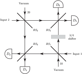
Figure 4: The experimental setup as described by Noh, Fougères and Mandel in Refs.Noh91 ; Noh92 .

Here we reconsider the calculation of some functions of the relative phase operator ${\hat{\phi}_{2}}-{\hat{\phi}_{1}}$ by making use of the PB-theory taking into account the post-selection mentioned above, i.e. disregarding measurements when the number of photons in detectors $D_{3}$ and $D_{4}$ and detectors $D_{5}$ and $D_{6}$ are equal. We therefore calculate all the expectation values within the PB scheme, by first evaluating the complete expectation value $\langle\cos^{n}(\hat{\phi}_{2}-\hat{\phi}_{1})\rangle$ according to Eq. (4) extended to two independent PB phase operators. We then subtract the contributions discarded by NFM in their experiment, i.e.

$$\lim_{s\rightarrow\infty}\sum_{m_{3}=0}^{s}\sum_{m_{4}=0}^{s}\sum_{m_{5}=0}^{s}\sum_{m_{6}=0}^{s}\langle m_{3}|\langle m_{4}|\langle m_{5}|\langle m_{6}|\,\rho\cdot\,$$

$$\cos^{n}(\hat{\phi}_{2}-\hat{\phi}_{1})|m_{6}\rangle|m_{5}\rangle|m_{4}\rangle|m_{3}\rangle\delta_{m_{3},m_{4}}\delta_{m_{5},m_{6}}$$ (26)

and renormalize the final result with the factor Noh91 ; Noh92 ; Noh92_2

$$N =1-e^{-(|\alpha_{1}|^{2}+|\alpha_{2}|^{2})}\,I_{0}\left(\frac{|\alpha_{1}^{2}-\alpha_{2}^{2}|}{2}\right)\,I_{0}\left(\frac{|\alpha_{1}^{2}+\alpha_{2}^{2}|}{2}\right)\ ,$$ (27)

where $I_{0}$ denotes a modified Bessel function. The initial density matrix $\rho$ has been assumed to be given by

$$\rho =|\alpha_{1}\rangle|\alpha_{2}\rangle|0\rangle_{1}|0\rangle_{2}\,\langle 0|_{2}\langle 0|_{1}\langle\alpha_{2}|\langle\alpha_{1}|\ ,$$ (28)

where the indices to the vacuum state indicates vacuum port 1 and 2 according to Figure 4. The normalizing factor $N$ as given in Eq.(27) is obtained by calculating the trace of this initial density matrix taking the post-selection condition into account. Input port 1 and 2 are in the coherent states $|\alpha_{1}\rangle$ and $|\alpha_{2}\rangle$ respectively with $\alpha_{1}=|\alpha_{1}|e^{i\xi_{1}}$ and $\alpha_{2}=|\alpha_{2}|e^{i\xi_{2}}$.

Figure 5: The expectation value $\langle\cos(\hat{\phi}_{2}-\hat{\phi}_{1})\rangle/\cos(\xi_{2}-\xi_{1})\approx\psi_{PB}({\bar{n}})$ according to the PB theory as a function of the average number of photons in the input port 1 using the experimental setup of Fig. 4. The input port 2 has a mean value ${\bar{n}}_{2}=50$ of photons. The SG-theory gives the same result which does not depend on the phase difference $\xi_{2}-\xi_{1}$. The NFM theory and NFM data curves are read from similar figures in Ref.Noh92 .

In Fig. 5 we present the result of the calculation of $\langle\cos({\hat{\phi}_{2}}-{\hat{\phi}_{1}})\rangle/\cos(\xi_{2}-\xi_{1})$ as a function of the average number of photons in port 1, i.e. ${\bar{n}}\equiv{\bar{n}}_{1}=|\alpha_{1}|^{2}$, for a fixed large average number of photons in port 2 ( ${\bar{n}}_{2}=|\alpha_{2}|^{2}=50$). As discussed in Refs.Noh91 ; Noh92 ; Noh92_2 the averages ${\bar{n}}_{1}$ and ${\bar{n}}_{2}$ should be replaced by the observed averages taking the experimental detection efficiency into account. Since ${\bar{n}}_{2}$ is large, the post-selection restriction above can be disregarded with an exponentially small error. Furthermore, the observable ${\hat{\phi}_{2}}$ can for sufficiently large ${\bar{n}}_{2}$ be replaced by $\xi_{2}$ and a straightforward calculation then leads to

$$\langle\cos({\hat{\phi}_{2}}-{\hat{\phi}_{1}})\rangle/\cos(\xi_{2}-\xi_{1})=\psi_{PB}({\bar{n}})~{}~{},$$ (29)

independent of $\xi_{2}-\xi_{1}$. We find that the PB-theory, which in this case agrees with the SG-theory, predicts results which lie above the experimental data as presented in Fig. 5. On this issue we are not in agreement with Ref.Noh92_2 since their corresponding curve lies below the experimental data. Our conclusion is, however, the same: due to the small error-bars the PB-theory does not agree with NFM experimental data in this case.

We now consider other observables considered in Refs.Noh91 ; Noh92 ; Noh92_2 but which were not calculated using the PB-theory. The expectation value $\langle\cos^{2}(\hat{\phi}_{1}-\hat{\phi}_{2})\rangle$ with the setup as given by Fig. 4, where the input port 2 is in a coherent state $|\alpha\rangle$ and the input port 1 is the vacuum field, is e.g. given by

$$\langle\cos^{2}(\hat{\phi}_{2}-\hat{\phi}_{1})\rangle =\frac{1}{2}~{}~{},$$ (30)

since the distribution $P(\phi_{1})$ for the observable ${\hat{\phi}_{1}}$ in this case is a constant and the averaging of the observable ${\hat{\phi}_{2}}$ with the post-selection of Fig. 4 leads to the normalization factor as given by Eq.(27). This result agrees exactly with the NFM theory and also with the experimental data as seen in Fig. 6. Even though the probability distributions of the relative phase in the PB and the NFM theory has been argued to be different in the NFM experimental situationNoh93 , some observables can nevertheless apparently lead to the same result. In a similar calculation of the corresponding expression using the SG-theory Carr68 we replace the $\cos^{2}(\hat{\phi}_{2}-\hat{\phi}_{1})$ PB operator by the square of the operator

$${\hat{C}}_{12}={\hat{C}}_{1}{\hat{C}}_{2}+{\hat{S}}_{1}{\hat{S}}_{2}~{}~{},$$ (31)

where the SG-theory operators ${\hat{C}}_{k}$ and ${\hat{S}}_{k}$ corresponds, for $k=1,2$, to the PG-theory operators $\cos(\hat{\phi}_{k})$ and $\sin(\hat{\phi}_{k})$ respectively. A calculation of $\langle{\hat{C}}_{12}^{2}\rangle$, making use of the definition Eq.(31) and with the conditions of Fig. 6 for a sufficiently large mean value ${\bar{n}}_{2}$ of photons in input port 2, i.e. when one can disregard effects of the NFM post-selection restriction mentioned above, then leads to the result

$$\langle{\hat{C}}_{12}^{2}\rangle=\frac{1}{4}(1-e^{-{\bar{n}}})~{}~{},$$ (32)

with an asymptotic value of $1/4$. As seen from Fig. 6 this asymptotic value is not in agreement with the NFM experimental data.

Figure 6: The figure compares the expectation values $\langle\cos^{n}(\phi-\phi_{0})\rangle$ evaluated with the PB theory and the NFM theory (NFMT) and experimental data (NFME) for $n=2$ and $n=4$ as a function of the number of quanta in input port 2 ($\bar{n}=|\alpha|^{2}$) according to Fig. 4 with a vacuum for input port 1.

The general expression of the expectation value $\langle\cos^{4}(\hat{\phi}_{2}-\hat{\phi}_{1})\rangle$ for the experimental setup as given by Fig. 4, where the input port 2 again is in a coherent state $|\alpha\rangle$ and the input port 1 is in the vacuum field, is given by

$$\langle\cos^{4}(\hat{\phi}_{2}-\hat{\phi}_{1})\rangle =\frac{3}{8}-\frac{T}{N}$$ (33)

where

$$T =\frac{3}{2}e^{-|\alpha|^{2}}\left\{-\frac{1}{12288}|\alpha|^{4}+A+B\right\}$$ (34)

with

$$A=\frac{1}{4}\sum_{m5=0}^{\infty}(\frac{1}{4}|\alpha|)^{2(m_{5}+3)}\frac{1}{(m_{5}+1)!^{2}}\cdot$$

$$\frac{m_{5}^{2}+2m_{5}-2}{\sqrt{{6(2m_{5}+3)(m_{5}+2)^{3}(2m_{5}+5)(m_{5}+3)^{3}}}}$$ (35)

and

$$B=~{}~{}~{}~{}~{}~{}~{}~{}~{}~{}~{}~{}~{}~{}~{}~{}~{}~{}~{}~{}~{}~{}~{}~{}~{}~{}~{}~{}~{}~{}~{}~{}~{}~{}~{}~{}~{}~{}$$

$$\frac{1}{8}\sum_{m3=0}^{\infty}\sum_{m5=0}^{\infty}(\frac{1}{4}|\alpha|)^{2(m_{3}+m_{5}+4)}\frac{1}{(m_{3}+2)!^{2}(m_{5}+2)!^{2}}\cdot$$

$$\frac{(m_{3}+m_{5}+4)(m_{3}+m_{5}+3)-4(m_{3}+2)(m_{5}+2)}{\sqrt{6(2m_{3}+2m_{5}+5)(m_{3}+m_{5}+3)}}\cdot$$

$$\frac{1}{\sqrt{(2m_{3}+2m_{5}+7)(m_{3}+m_{5}+4)}}~{}.~{}~{}~{}~{}~{}~{}~{}~{}$$ (36)

A very accurate analytical approximation of this expression is

$$\langle\cos^{4}(\hat{\phi}_{2}-\hat{\phi}_{1})\rangle\approx~{}~{}~{}~{}~{}~{}~{}~{}~{}~{}~{}~{}~{}~{}~{}~{}~{}~{}~{}~{}~{}~{}~{}~{}~{}\,$$

$$\frac{3}{8}+\frac{3}{2}\,e^{-|\alpha|^{2}}\,\left({\frac{1}{12288}|\alpha|^{4}+\frac{\sqrt{15}}{4423680}|\alpha|^{6}}\right)/N~{}~{}~{}.$$ (37)

For small values of $|\alpha|^{2}$, ($\,|\alpha|^{2}\leq 1$), we also find that

$$\langle\cos^{4}(\hat{\phi}_{2}-\hat{\phi}_{1})\rangle\approx\frac{3}{8}+\frac{1}{8192}|\alpha|^{2}+\frac{1}{65546}(\frac{\sqrt{15}}{45}-3)|\alpha|^{4}~{}~{}~{},$$ (38)

is an accurate analytical approximation with an error of less than $1\%$.

Figure 7: The expectation value $\langle\cos^{4}(\phi-\phi_{0})\rangle$ evaluated with the PB theory as a function of $\bar{n}=|\alpha|^{2}$ with the NFM post-selection condition included as described in the main text. The experimental setup is as in Fig. 6.

In Fig. 6 we compare the expectation values $\langle\cos^{n}(\hat{\phi}_{2}-\hat{\phi}_{1})\rangle$ with $n=2$ and $n=4$ of the PB theory with NFM data and theory. As we noticed above, for $n=2$ the curves overlap, but with $n=4$ the curves are completely different. The theoretical PB curve for $n=4$ is actually very close to the constant $\frac{3}{8}$ for all values of ${\bar{n}}$. The effect of the post-selection is not visible in Fig. 6. In Fig. 7 we have enlarged the portion of Fig. 6 where the post-selection is important and it is seen that the NFM post-selection only leads to a very small numerical correction for ${\bar{n}}\leq 10$.

As we see in Fig. 8 the values of phase fluctuations found from the PB theory are in good agreement with the experimental results of GBL. We also notice that NFM data and theory lie at the edge of the accepted variance of the GBL data. The GBL experimental data have here been adjusted to apply to the experimental setup as presented in Fig. 4. In contrast to the GBL experimental procedure we now do not have two independent measurements. The necessary adjustments are a division of $2$ of the GBL data and a corresponding division by $\sqrt{2}$ of the variances as quoted by GBL Gerhardt74 .

Figure 8: This figure compares the relative phase variance $(\Delta\cos({\hat{\phi}_{1}}-{\hat{\phi}_{2}}))^{2}+(\Delta\sin({\hat{\phi}_{1}}-{\hat{\phi}_{2}}))^{2}$ evaluated with the PB theory and the corresponding NFM theory variance $\langle(\Delta\hat{C}_{M})^{2}\rangle+\langle(\Delta\hat{S}_{M})^{2}\rangle$, the NFM data of Ref.Noh92 and the GBL data from Ref.Gerhardt74 . The conditions are as described in Fig. 5. In addition horizontal error-bars of width $\bar{n}^{1/2}$ are added to the GBL data.

The NFM experimental data as well as the NFM theoretical values used in the figures of the present paper are read from the corresponding figures in the article Noh92 by importing the relevant figures and making use of a graphical and computer-based numerical routine with a sufficient numerical accuracy.

VI FINAL REMARKS

In summary, we have reconsidered some aspects of quantum operator phase theories and recalculated various expectation values of relative phase operators using in particular the PB-theory and, with regard to the NFM experimental data, we have taken appropiate post-selection constraints into account when required. We have also considered a set of observables which has been measured but not previously calculated using the PB-theory. We have seen that there are definitions of phase fluctuations which do not depend on the actual phases of coherent states used to describe the quantum states to be probed, even though the purity of the states are important. The PB-theory appears to describe accurately some experimental data but not all. Some of our results are in disagreement with similar results available in the literature but we, nevertheless, reach a similar conclusion as in the NFM theory Noh91 ; Noh92 ; Noh92_2 , i.e. the notion of a relative quantum phase depends on the actual experimental setup. We have limited our considerations to the GBL Gerhardt74 - and the NFM Noh91 ; Noh92 ; Noh92_2 - experimental data. Further experimental considerations has been discussed in e.g. Ref.Torgerson96 , and commented upon in Ref.Font02 , illustrating again that the notion of a relative quantum phase appears to depend on the experimental situation.

ACKNOWLEDGMENT

One of the authors (B.-S.S.) wishes to thank NorFA for financial support and Göran Wendin and the Department of Microelectronics and Nanoscience at Chalmers University of Technology and Göteborg University for hospitality. The authors also which to thank a referee for several constructive remarks.

References

- (1) P. Carruthers and M. M. Nieto, “Phase and Angle Variables in Quantum Mechanics”, Rev. Mod. Phys. 40, 411 1968.
- (2) “Quantum Phase and Phase Dependent Measurements”, Eds. W. P. Schleich and S. M. Barnett, Physica Scripta T48 (1993).
- (3) S. M. Barnett and P. M. Radmore, “Methods in Theoretical Quantum Optics” (Clarendon Press, Oxford, 1997).
- (4) R. Lynch, “Fluctuations of the Barnett-Pegg Phase Operator in a Coherent State”, Phys. Rev. A 41, 2841 (1990). Also see “The Quantum Phase Problem: A Critical Review”, Phys. Rep. 256 367 (1995).
- (5) C. C. Gerry and K. E. Urbanski, “Hermitian Phase-Difference Operator Analysis of Microscopic Radiation-Field Measurement”, Phys. Rev. A 42, 662 (1990).
- (6) S. M. Barnett and D. T. Pegg , “Phase in Quantum Optics”, J. Phys. A 19, 3849 (1986); “On the Hermitian Optical Phase Operator”, J. Mod. Opt. 36, 7 (1989); “Phase Properties of the Quantized Single-Mode Electromagnetic Field”, Phys. Rev. A 39, 1665 (1989).
- (7) H. Gerhardt, H. Welling and D. Fröhlich, “Ideal Laser Amplifier as a Phase Measuring System of a Microscopic Radiation Field”, Appl. Phys. 2, 91 (1973); H. Gerhardt, U. Büchler and G. Lifkin, “Phase Measurement of a Microscopic Radiation Field”, Phys. Lett. 49A, 119 (1974)
- (8) M. Orzag, “Quantum Optics” (Springer, 2000).
- (9) J. R. Klauder and B.-S. Skagerstam, “Coherent States-Applications in Physics and Mathematical Physics ” (World Scientific, Singapore, 1985 and Beijing 1988); B.-S. Skagerstam, “Coherent States - Some Applications in Quantum Field Theory and Particle Physics ” in “Coherent States: Past, Present, and the Future ”, Eds. D. H. Feng, J. R. Klauder and M. R. Strayer (World Scientific, Singapore, 1994).
- (10) K. Mølmer, “Quantum Entanglement and Classical Behaviour”, J. Mod. Opt. 44, 1937 (1997) and “Optical Coherence: A Convenient Fiction”, Phys. Rev. A 55, 3195 (1997).
- (11) M. O. Scully and M. S. Zubairy, “Quantum Optics ” (Cambridge University Press, Cambridge, 1996).
- (12) S. J. van Enk and C. A. Fuchs, “Quantum State of an Ideal Propagating Laser Field”, Phys. Rev. Lett. 88 027902-1 (2002) and “The Quantum State of a Laser Field”, Quantum Inf. Comput. 2 1551 (2002); S. J. van Enk “Phase Measurements With Weak Reference Pulses”, Phys. Rev. A 66 042308 (2002).
- (13) J. Gea-Banacloche, “Comment on “Optical Coherence: A Convenient Fiction””, Phys. Rev. A 58, 4244 (1998) and “Emergence of Classical Radiation Fields Through Decoherence in the Scully-Lamb Laser Model”, Foundations of Physics 28, 531 (1998).
- (14) G. G. Paulus, F. Grasbon, H. Walther,H P. Villoresi, M. Nisoli, S. Stagira, E. Prioro and S. De Silvestri, “Absolute-Phase Phenomena in Photoinonization With Few-Cycle Laser Pulses”, Nature 414 182 (2001).
- (15) L. Susskind and J. Glogower, “Quantum Mechanical Phase and Time Operator”, Physics 1, 49 (1964).
- (16) J. W. Noh, A. Fougères and L. Mandel, “ Measurement of the Quantum Phase by Photon Counting”, Phys. Rev. Lett. 67, 1426 (1991).
- (17) J. W. Noh, A. Fougères and L. Mandel, “Operational Approach to the Phase of a Quantum Field”, Phys. Rev. A45, 424 (1992).
- (18) J. W. Noh, A. Fougères and L. Mandel, “Further Investigations of the Operationally Defined Quantum Phase”, Phys. Rev. A46, 2840 (1992).
- (19) See e.g. Yu. I. Vorontsov and Yu. A. Rembovsky, “The Problem of the Pegg-Barnett Phase Operator”, Phys. Rev. A254, 7 (1999) and K. Kakazu, “Extended Pegg-Barnett Phase Operator”, Prog. Theor. Phys. 106, 721 (2001) .
- (20) J. H. Shapiro and S. H. Shepard, “Quantum Phase Measurement: A System-Theory Perspective”, Phys. Rev. A43, 3795 (1991).
- (21) M. Bouten, N. Maene and P. Van Leuven, “On an Uncertainty Relation for Angular Variables”, Nuovo Cim. 37 1119 (1965).
- (22) D. Judge , “On the Uncertainty Relation for Angle Variables”, Nuovo Cim. 31 332 (1964).
- (23) M. M. Nieto, “Phase-Difference Operator Analysis of Microscopic Radiation-Field Measurements”, Phys. Lett. 60A, 401 (1977).
- (24) J. W. Noh, A. Fougères and L. Mandel, “Measurements of the Probability Distribution of the Operational Defined Quantum Phase Difference”, Phys. Rev. Lett. 71, 2579 (1993).
- (25) J. R. Torgerson and L. Mandel, “Is there a Unique Operator for the Phase Difference of Two Quantum Fields?”, Phys. Rev. Lett. 76, 3939 (1996).
- (26) M. Fontenelle, S. L. Braunstein, W. P. Schleich and M. Hillery, “Direct and Indirect Strategies for Phase Measurement”, Acta Physica Slovaca 46, 373 (1996) and in quant-ph/9712032 (1997).