On a suggestion relating topological and quantum mechanical entanglements
M. Asoudeh,       V. Karimipour ,       L. Memarzadeh,

A. T. Rezakhani

Department of Physics, Sharif University of Technology,

P.O. Box 11365-9161,

Tehran, Iran

We analyze a recent suggestion [2, 3] on a possible relation between topological and quantum mechanical entanglements. We show that a one to one correspondence does not exist, neither between topologically linked diagrams and entangled states, nor between braid operators and quantum entanglers. We also add a new dimension to the question of entangling properties of unitary operators in general.

Figure 1: A knot representation of the disentangled state $|\phi\rangle\otimes|\psi\rangle$.

Figure 2: A knot representation of a bipartite entangled state.

1 Introduction

In a recent series of papers [1, 2, 3], it has been argued that there may be a relation between quantum mechanical entanglement and topological entanglement. This hope has been raised by some formal similarities between entanglement of quantum mechanical states which is an algebraic concept and linking of closed curves which is a topological concept. Let us begin by simple definitions of these two concepts and the basic idea of a correspondence put forward in the above papers.
A pure quantum state of a composite system $AB$ (a vector $|\Psi\rangle$ in the tensor product of two Hilbert spaces ${\cal{H}}_{A}\otimes{\cal{H}}_{B}$) is called entangled if it can not be written as a product of two vectors , i.e. $|\Psi\rangle\neq|\psi\rangle_{A}\otimes|\phi\rangle_{B}$. The simplest entangled pure states occur when ${\cal{H}}_{A}$ and ${\cal{H}}_{B}$ are two dimensional with basis vectors $|0\rangle$ and $|1\rangle$, called a qubit in quantum computation literature. For brevity in the following we will not write the subscripts $A$ and $B$ explicitly. A general state of two qubits

$$|\Psi\rangle=a|0,0\rangle+b|0,1\rangle+c|1,0\rangle+d|1,1\rangle$$ (1)

is entangled provided $ad-bc\neq 0$.
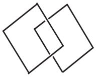
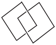
On the other hand two curves can be in an unlinked position like the one shown in figure (1) or in a linked position like the one shown in figure (2). One is tempted to view the two unlinked curves as a topological representation of a disentangled quantum state and the two linked curves as a representation of an entangled state.
In the same way that cutting any of the curves in figure (2) removes the topological entanglement, measuring one of the qubits of the state $|\Psi\rangle$ in (1) in any basis (not necessarily the $\{|0\rangle,|1\rangle\}$ basis), disentangles the quantum state.
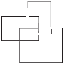
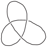
More evidence in favor of this analogy is provided by figure 3 [3], which provides an alleged topological equivalent for the so-called GHZ state [4]

$$|{\rm{GHZ}}\rangle:=\frac{1}{\sqrt{2}}(|0,0,0\rangle+|1,1,1\rangle).$$ (2)

In this figure cutting any of the three curves, leaves the other two curves in an unlinked position, in the same way that measuring any of the three subsystems in the GHZ state in the $\{|0\rangle,|1\rangle\}$ basis, leaves the other two subsystems in a disentangled state.
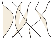
One may be tempted to make a general correspondence between topologically linked diagrams and entangled states or vice versa. For example while figure 3 corresponds to the GHZ state, a slight modification of the crossings of this link diagram, as shown in figure 4, may correspond to the following state

$$|\Phi\rangle=\frac{1}{2}(|0,0,0\rangle+|1,1,0\rangle+|1,0,1\rangle+|0,1,1\rangle).$$ (3)

Figure 3: A knot representation of the GHZ state $\frac{1}{\sqrt{2}}(|0,0,0\rangle+|1,1,1\rangle)$, known also as Borromean rings.

Figure 4: A knot representation of the entangled state $|\Phi\rangle=\frac{1}{2}(|0,0,0\rangle+|1,1,0\rangle+|1,0,1\rangle+|0,1,1\rangle)$.

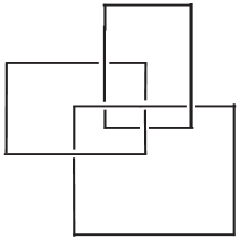
If one measures one of the subsystems in this state in the $\{|0\rangle,|1\rangle\}$ basis, the other two subsystems are projected onto an entangled state, in the same way that cutting out any of the component curves in figure 4 leaves the other two components in a linked position.

A natural question arises as to how serious and deep such a correspondence may be. Certainly such a relation, if exists, will be much fruitful for both fields and it is worthwhile to explore further the possibility of its existence. We should stress here that we only want to analyze one particular suggestion [2, 3], regarding a possible correspondence between topological and quantum mechanical entanglement. We are not concerned here with other aspects of the relation between topology and quantum computation or quantum mechanics. These avenues of study have been followed in [5, 6, 7, 8] where the possibility of doing fault tolerant quantum computation by using topological degrees of freedom of certain systems with anyonic excitations or the design of quantum algorithms for calculating topological invariants of knots are analyzed.

It is the aim of this paper to shed more light on these analogies and to study more closely the similarities and differences between these the above types of entanglement. The overall picture that we obtain is that these analogies do not point to a deep relation between these concepts, since despite some superficial similarities, there are many serious differences which lead to the conclusion that such a correspondence can not be taken seriously.

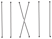
Here we list some of these differences.

1- If we want to correspond any component of a linked knot with a state of a vector space in a tensor product space, (the number of vector spaces being equal to the number of components of the link diagram), then we are faced with the obvious question of ”What kind of state corresponds to a knot which is highly linked with itself”. We can imagine many topologically different one component knots and yet we have to correspond them all to a single state in a vector space which necessarily has no self-entanglement. Figure (5) shows such a knot known as trefoil knot.
One way out is to consider only linked diagrams whose individual components have no self linking and to take into account the linking between different components. But there is no natural way to separate the linking of a component with itself from that with others. A component may be topologically trivial by itself (when one removes all the other components), but can not be deformed continuously to a trivial knot due to the presence of other components.

Figure 5: The trefoil knot, an example of a single component knot which is entangled.

2- The second problem is that quantum entanglement should not change by local unitary operations which is equivalent to local change of basis. Therefore for such a correspondence to be valid, two quantum mechanical states which are related to each other by local unitary operations should correspond to topologically equivalent diagrams. Let us see if this is the case. Consider the examples given above: The two states (2) and (3) are related to each other by the local action of three Hadamard matrices ($H:={\frac{1}{\sqrt{2}}\left(\begin{array}[]{cc}1&1\\ 1&-1\end{array}\right)}$):

$$|{\rm{GHZ}}\rangle=H\otimes H\otimes H|\Phi\rangle\hskip 28.45274pt|\Phi\rangle=H\otimes H\otimes H|{\rm{GHZ}}\rangle$$ (4)

and yet they correspond to completely inequivalent diagrams, shown in figures 3 and 4, respectively.

3- The third problem concerns the alleged relation between ”measurement” of a quantum state on one hand and ”cutting a line” in a knot diagram on the other hand. This relation is very questionable. The only evidence is that in some simple cases as those mentioned above, it appears that measurement (reduction) of a state $|\Psi\rangle$ which corresponds to a knot $K$, produces a state $|\Psi^{\prime}\rangle$ which corresponds to a knot $K^{\prime}$ obtained by cutting one of the lines of $K$. However this correspondence is too superficial since the reduction of a wave function depends on what value we obtain for our observable while cutting a line is an action with a unique and predetermined result. To see this more explicitly consider a state like

$$|W\rangle=\frac{1}{\sqrt{3}}(|1,0,0\rangle+|0,1,0\rangle+|0,0,1\rangle).$$ (5)

If we measure the first qubit in the computational basis $\{|0\rangle,|1\rangle\}$ and obtain the value $0$, the other two qubits are projected onto an entangled state, while if we obtain the value $1$, the other two qubits are projected onto a disentangled state. Therefore one can not identify a measurement with a simple cutting of a line in a knot diagram. The result of the measurement also determines if the remaining state is entangled or not.
These examples provide sufficient reasons to abandon the kind of correspondence mentioned above. But the question of a possible relation remains open and there may be an alternative and more tractable framework for studying it.
It is well known that all knots and links can be obtained from closure of braids, the latter having a direct relation with operators acting on tensor product spaces. Therefore it may be possible to find a correspondence between entangling operators on the quantum mechanical side and braid operators which produce topological entanglement on the other side. It is in order to present a short review of braid group and braid operators.

1.1 A review of braid group

A braid on $n$ strands (figure 6) is the equivalence class of a collection of continuous curves joining $n$ points in a plane to $n$ similar points on a plane on top of it. The curves should not intersect each other but can wind around each other arbitrarily.

Figure 6: A braid on 6 strands, an element of the group $B_{6}$.

Two collections of curves which can be continuously deformed to each other are considered equivalent. There is a well-known theorem stating that each knot can be constructed from the closure of a braid (see [9] for a review). By closure of a braid we mean joining the points on the lower plane to those on the upper one by continuous lines which lie outside all the curves of the braid.
The collection of all braids can be equipped with a group structure by defining the product of two braids $\alpha$ and $\beta$ as the equivalence class of a braid obtained by inserting the braid $\beta$ on top of the braid $\alpha$. The unit element of this group is simply the equivalence class of paths which do not wind around each other when they go from the lower plane to the upper one.
This group, called the braid group on $n$ strands and denoted by $B_{n}$, is generated by the simple braids $\sigma_{i}$, $i=1,\ldots,n-1$, shown in figure 7, where each $\sigma_{i}$ intertwines, only once, the strands $i$ and $i+1$ ( $\sigma_{i}^{-1}$ intertwines the strands in the opposite direction). Such elements generate the whole braid group when supplemented with the following relations which express topological equivalence of braids as the reader can verify:

$$\sigma_{i}\sigma_{i+1}\sigma_{i} = \sigma_{i+1}\sigma_{i}\sigma_{i+1}$$ (6)

$$\sigma_{i}\sigma_{j} = \sigma_{j}\sigma_{i}\ \ \ \ {\rm{if}}\ \ \ |i-j|\geq 2.$$ (7)

The expression of braids as elements of a group shows how to find the inverse of braids as topological objects. For example the inverse of $\alpha=\sigma_{1}\sigma_{2}$ is $\alpha^{-1}=\sigma_{2}^{-1}\sigma_{1}^{-1}$.
One can obtain a representation of the braid group $B_{n}$ for any $n$ on the tensor product space $V^{\otimes n}$, if one can find a solution of the following equation in $V^{\otimes 3}$ called hereafter the braid relation

$$(R\otimes I)(I\otimes R)(R\otimes I)=(I\otimes R)(R\otimes I)(I\otimes R),$$ (8)

in which $R:V\otimes V\rightarrow V\otimes V$ is a linear operator called a braid operator and $I$ is the identity operator. Once such a solution is found, representations of generators of the braid group and hence the whole braid group is obtained as follows:

$$\sigma_{i}=I^{\otimes^{i-1}}\otimes R\otimes I^{\otimes^{n-i-1}}$$ (9)

where for simplicity we have used the same notation for $\sigma_{i}$ and its representation.
Thus if we have a braid operator $R$, we can produce representations of all kinds of braids with all the variety of their topological entanglement.
Once a representation is in hand one can try to construct invariants of knots by defining suitable traces on the space $V^{\otimes n}$ [10].
We have now set the stage for asking the question of a possible relation between topological and quantum mechanical entanglement in an appropriate way. We can ask the following questions:

1- Does every braid operator which produces topological entanglement, also necessarily produces quantum entanglement? or conversely

2- Does every quantum entangler (an operator which entangles product states) necessarily produces topological entanglement?, that is , is any quantum entangler related somehow to a solution of the braid group relation?

We think that the answer to these questions will shed light on the question of relation between topological and quantum mechanical entanglements.
We choose to investigate these questions for two dimensional spaces, since in two dimensions we have both a classification of solutions of the braid group relation and a great deal of information about measures of quantum entanglement.
In the rest of this paper we try to answer the above questions and draw our conclusions which are mainly negative, that is we conclude that the two types of entanglement may not be related to each other in such a direct way. This however does not exclude the possibility that quantum computation may someday be used for calculating topological invariants of knots [5, 6, 7].

Figure 7: The generator $\sigma_{3}$ of the braid group $B_{6}$.

The structure of this paper is as follows. In section 2 we present all the unitary solutions of the braid group relation in two dimensions (4$\times$4 unitary braid operators $R$). In section 3 we collect the necessary tools for the analysis of entanglement of states and entangling properties of operators. In section 4 we use these tools to characterize the braid operators. Finally we end the paper with a discussion which encompasses a summary of our results.

2 All unitary braid operators in two dimensions

Let $V$ be a vector space and let $\hat{R}:V\otimes V\rightarrow V\otimes V$ be a linear operator. The following equation which is a relation between operators acting on $V\otimes V\otimes V$ is called the Yang-Baxter relation first formulated in studies on integrable models [11]

$$\hat{R}_{12}\hat{R}_{13}\hat{R}_{23}=\hat{R}_{23}\hat{R}_{13}\hat{R}_{12},$$ (10)

where the indices indicate on which of the three spaces, the operator is acting non-trivially. Any solution $\hat{R}$ of the Yang-Baxter equation provides a braid operator $R$ by the simple relation $R=P\hat{R}$, where $P$ is the permutation or SWAP operator defined as $P|i,j\rangle=|j,i\rangle$. When the vector space $V$ is two dimensional, the solutions of Yang-Baxter equation have been classified up to the symmetries allowed by the equation [12, 13, 14]. From these solutions we can select those solutions of the braid group equation which are unitary. We should stress that this restriction can be relaxed and one can also consider non-unitary solutions of braid group. The reason for our interest in unitary operators in this paper is that in quantum mechanics we want to use these operators as quantum gates.
There are only two types of unitary solutions. A single one designated as

$$\hskip 28.45274ptR=\frac{1}{\sqrt{2}}\left(\begin{array}[]{cccc}1&&&1\\ &1&-1&\\ &1&1&\\ -1&&&1\end{array}\right)$$ (15)

and a continuous family of solutions

$$R^{\prime}=\left(\begin{array}[]{cccc}a&&&\\ &&b&\\ &c&&\\ &&&d\end{array}\right),$$ (20)

where the complex parameters $a,b,c,$ and $d$ are pure phases, i.e. $|a|=|b|=|c|=|d|=1$.
Note that the SWAP operator (denoted by $P$) is a special kind of the matrix $R^{\prime}$ for which $a=b=c=d=1$. For general value of its parameters, it is simply the SWAP operator times a diagonal matrix. The second of these solutions can be generalized to arbitrary dimensions, in the form $R^{\prime}_{ij,kl}=M_{ij}\delta_{il}\delta_{jk}$, where $|M_{ij}|=1$. We do not know of any generalizations of the other solution.

3 Entanglement of pure states and entangling power of unitary operators

Consider a pure state of two qubits $A$ and $B$:

$$|\Psi\rangle_{AB}=\alpha|0,0\rangle+\beta|0,1\rangle+\gamma|1,0\rangle+\delta|1,1\rangle.$$ (21)

The single parameter

$$C:=2|\alpha\delta-\beta\gamma|$$ (22)

called the concurrence, characterizes the entanglement of this state [15, 16]. For a product state $|\psi\rangle\otimes|\psi^{\prime}\rangle\equiv(x|0\rangle+y|1\rangle)\otimes(x^{\prime}|0\rangle+y^{\prime}|1\rangle),$ this parameter is zero and for a maximally entangled state like one of the Bell states $(\frac{|0,0\rangle\pm|1,1\rangle}{\sqrt{2}},\frac{|0,1\rangle\pm|1,0\rangle}{\sqrt{2}})$, it takes its maximum value of 1. We note that the concurrence can be written as $C=|\langle\Psi^{*}|\sigma_{y}\otimes\sigma_{y}|\Psi\rangle|$ where $\sigma_{y}$ is the second Pauli matrix and $*$ denotes complex conjugation in the computational basis. This also shows that the concurrence is invariant under local transformations $|\Psi\rangle\rightarrow U\otimes V|\Psi\rangle$, since $U^{T}\sigma_{y}U=\sigma_{y}$.
Any other measure of entanglement, like the von Neumann entropy of the reduced density matrices $\rho_{A}$ or $\rho_{B}$ defined as

$$E_{v}(\rho):=-{\rm tr}(\rho\ln\rho)$$

or the linear entropy defined as

$$E_{l}(\rho):=1-{\rm tr}(\rho^{2})$$

can be expressed in terms of this parameter. A simple calculation shows that the eigenvalues of the reduced density matrix for the state in (21) are

$$\lambda_{\pm}=\frac{1}{2}(1\pm\sqrt{1-C^{2}}),$$ (23)

from which the simple expression $E_{l}=\frac{1}{2}C^{2}$ is obtained for the linear entropy.
The concurrence, the linear entropy or the von Neumann entropy are increasing functions of each other, all of them vanish for a product state and take their maximum values of $1$, $\frac{1}{2}$ and $1$ respectively for maximally entangled states. One can use any of these measures for the characterization of entanglement of a pure state of two qubits.
So much for the entanglement properties of states, we now turn to the entangling properties of operators acting on the space of two qubits.
The space of unitary operators acting on two qubits (the group U(4)) when viewed in terms of entangling properties has a rich structure. Those in the subgroup U(2)$\otimes$U(2) are called local operators. Elements of this subgroup can not produce entangled states when acting on product states. The complement of this subgroup forms the set of non-local operators. In the set of non-local operators, those which can produce a maximally entangled state when acting on a suitable product state are called perfect entangler [17]. An example in this class is the CNOT operator defined as ${\rm{CNOT}}|i,j\rangle=|i,i+j~{}({\rm{mod}}\ 2)\rangle$. Those non-local operators which do not have this property are called non-perfect entanglers. Note also that there are non-local operators which can not produce any entanglement at all. An example is the SWAP operator $P$ which is incidentally a braid group operator.
An important concept is the local equivalence of two operators. Let two operators $U$ and $U^{\prime}$ in U(4) be related as follows:

$$U^{\prime}=(k\otimes l)U(k^{\prime}\otimes l^{\prime}),$$ (24)

where the local operators $k,l,k^{\prime},l^{\prime}\in{\rm U(2)}$. Two such operators should be regarded equivalent as far as their entangling properties are concerned.
As far as entangling properties are concerned one may extend this notion of equivalence to the case where the two operators are related by the SWAP operator $P$, that is when $U^{\prime}=UP$ or $U^{\prime}=PU$, or both, since the SWAP operator does not change the entanglement of a state. However the SWAP operator is non-local which means that it can not be implemented by local unitary operations on the two states. Moreover as far as topological properties are concerned, the SWAP operator is a braid operator and totally changes the topological class of a braid. For this reason we restrict ourselves to the notion of bi-local equivalence as in (24).

How can we find if two such operators are equivalent? This question has been studied by many authors [18, 19, 20, 21, 17]. The orbits of states under bi-local [21, 17] and multi-local unitaries (in the case of multi-particle states) [19, 20] have been characterized by certain invariants. Here we use the invariants found in [21, 17]. Let us define the matrix $Q$ as follows:

$$Q=\frac{1}{\sqrt{2}}\left(\begin{array}[]{cccc}1&0&0&i\\ 0&i&1&0\\ 0&i&-1&0\\ 1&0&0&-i\end{array}\right).$$ (29)

For any matrix $U\in{\rm U(4)}$ define the following matrix:

$$m(U):=(Q^{\dagger}UQ)^{T}(Q^{\dagger}UQ)$$ (30)

where $T$ denotes the transpose. Note that $Q^{\dagger}UQ$ is nothing but the matrix expression of the operator $U$ in the Bell basis modulo some phases. It is shown in [21, 17] that the followings are invariant under bi-local unitary operations:

$$G_{1}~{}=~{}\frac{{\rm tr}^{2}[m(U)]}{16\det U}$$ (31)

$$G_{2}~{}=~{}\frac{{\rm tr}^{2}[m(U)]-{\rm tr}[m^{2}(U)]}{4\det U}.$$ (32)

3.1 Perfect entanglers

By a perfect entangler we mean an operator which can produce maximally entangled states when acting on a suitable product state. The following theorem [17] determines when a given operator $U\in{\rm U(4)}$ is a perfect entangler.

Theorem [17]: An operator $U\in{\rm U(4)}$ is a perfect entangler if and only if the convex hull of the eigenvalues of the matrix $m(U)$ contains zero.
We remind the reader that the convex hull of $N$ points $p_{1},p_{2},\cdots,p_{N}$ in $\texttt{R}^{n}$ is the set

$${\cal C}:=\{\sum_{j=1}\lambda_{j}p_{j}|\lambda_{j}\geq 0\ \ {\rm{and}}\ \ \sum_{j=1}^{N}\lambda_{j}=1\}.$$ (33)

The above criterion divides the set of non-local operators into perfect entanglers and non-perfect entanglers. A more quantitative measure has been introduced in [22] which defines the entangling power of an operator $U$, as

$$e_{p}(U):=\overline{E(U|\phi\rangle\otimes|\psi\rangle)},$$ (34)

where $E$ is any measure of entanglement of states and the average is taken over all product states. To guarantee that the entangling power of equivalent operators are equal, as it should be, the measure of integration is taken to be invariant under local unitary operations.

Equipped with the above tools we can now repose the questions raised in the introduction and ask what are the status of the braid group solutions in the space of all operators acting on two qubits. Which of them is a perfect entangler? If yes, are they both equivalent to some well-known perfect entanglers like CNOT or else, they belong to different equivalence classes of perfect entanglers? In answering these questions we have found some new features of entangling properties of operators as we will discuss in the sequel.

4 Entangling properties of braid operators

In this section we want to study the entangling property of the braid operators (15,20). Before proceeding we note a point without any calculation. The SWAP operator is a braid operator, (it is equal to $R^{\prime}$ when $a=b=c=d=1$) and yet it can not entangle product states. In fact $P(|\phi\rangle\otimes|\psi\rangle)=|\psi\rangle\otimes|\phi\rangle$. On the other hand the operator CNOT is not a solution of braid group relation and yet it is a perfect entangler. In fact when acting on the product states

$$\frac{1}{\sqrt{2}}(|0\rangle+|1\rangle)\otimes|0\rangle,\hskip 28.45274pt\frac{1}{\sqrt{2}}(|0\rangle+|1\rangle)\otimes|1\rangle$$ (35)

$$\frac{1}{\sqrt{2}}(|0\rangle-|1\rangle)\otimes|0\rangle,\hskip 28.45274pt\frac{1}{\sqrt{2}}(|0\rangle-|1\rangle)\otimes|1\rangle$$ (36)

it produces the maximally entangled Bell states

$$\frac{|0,0\rangle+|1,1\rangle}{\sqrt{2}},\hskip 28.45274pt\frac{|0,1\rangle+|1,0\rangle}{\sqrt{2}}$$ (37)

$$\frac{|0,0\rangle-|1,1\rangle}{\sqrt{2}},\hskip 28.45274pt\frac{|0,1\rangle-|1,0\rangle}{\sqrt{2}}.$$ (38)

However by this example we do not want to rush to the conclusion that there is absolutely no relation between braid operators and quantum mechanical entangling operators. The reason is that although the operator CNOT may not be a braid operator itself, it may be locally equivalent to a braid operator via bi-local unitary operators.
Therefore to study the entangling properties of braid operators we have to extract their non-local properties which is achieved by first calculating their invariants. For comparison we note that the invariants of CNOT turn out to be $G_{1}=0,$ and $G_{2}=1$.

1: For the braid operator $R$ we have:

$$m(R)=-i\left(\begin{array}[]{cccc}&&&1\\ &&1&\\ &1&&\\ 1&&&\end{array}\right)$$ (43)

from which we obtain the invariants

$$G_{1}(R)=0\hskip 28.45274ptG_{2}(R)=1.$$ (44)

These invariants are the same as the invariants of CNOT, and hence this braid operator is equivalent to a quantum mechanical perfect entangler. It is readily seen from (15) that when acting on the computational basis $\{|0,0\rangle,|0,1\rangle,|1,0\rangle,|1,1\rangle\}$ it produces the Bell basis.

2: For the continuous family $R^{\prime}$ we obtain after simple calculations

$$m(R^{\prime})={\rm{diag}}(ad,bc,bc,ad)$$ (45)

This leads to the invariants

$$G_{1}(R^{\prime}) = \frac{-(ad+bc)^{2}}{4abcd}\equiv-\frac{(1+\Delta)^{2}}{4\Delta}$$ (46)

$$G_{2}(R^{\prime}) = -1+2G_{1},$$ (47)

where $\Delta:=\frac{ad}{bc}$.
The last relation $G_{2}=-1+2G_{1}$ shows that none of the members of this family is equivalent to CNOT. In fact they are not equivalent to any controlled operator $U_{c}$ (such an operator acts on the second qubit as $U$ only if the first qubit called the control qubit is in the state $|1\rangle$, otherwise it acts as a unit operator). In fact a simple calculation shows that for all such controlled operators we have

$$G_{2}(U_{c})=1+2G_{1}(U_{c}).$$ (48)

which means that even if the first invariant of such an operator is made equal to that of $R^{\prime}$, their second invariants can not be equal to each other and thus under no condition the braid operator $R^{\prime}$ can be locally equivalent to a controlled operator $U_{c}$.

Now that none of these braid operators are equivalent to CNOT, is there any perfect entangler among them?

To answer this question we note that the eigenvalues of the matrix $m(R^{\prime})$ are $ad$ and $bc$. The convex hull of these points in the complex plane is a line which passes through the origin only if the parameter $\Delta$ is real. Since all the parameters $a,b,c$ and $d$ are of unit modulus, this parameter can only have two values, namely $\pm 1$. The value $\Delta=1$ should be excluded, since in that case the eigenvalues are all equal and the convex hull degenerates to a point. Thus the braid operators $R^{\prime}$ are perfect entanglers only if $\Delta=-1$. Since this same parameter determines the invariants of $R^{\prime}$, there is only one single perfect entangler in this class up to local equivalence. We take this perfect entangler to be the following matrix with invariants $G_{1}=0$ and $G_{2}=-1$:

$$R^{\prime}_{0}:=\left(\begin{array}[]{cccc}1&&&\\ &&1&\\ &-1&&\\ &&&1\end{array}\right).$$ (53)

It produces maximally entangled states when acting on an appropriate product basis:

$$R^{\prime}_{0}|x+\rangle|x+\rangle=\frac{1}{2}(|0,0\rangle+|0,1\rangle-|1,0\rangle+|1,1\rangle)$$ (54)

$$R^{\prime}_{0}|x+\rangle|x-\rangle=\frac{1}{2}(|0,0\rangle+|0,1\rangle+|1,0\rangle-|1,1\rangle)$$ (55)

$$R^{\prime}_{0}|x-\rangle|x+\rangle=\frac{1}{2}(|0,0\rangle-|0,1\rangle-|1,0\rangle-|1,1\rangle)$$ (56)

$$R^{\prime}_{0}|x-\rangle|x-\rangle=\frac{1}{2}(|0,0\rangle-|0,1\rangle+|1,0\rangle+|1,1\rangle)$$ (57)

where $|x\pm\rangle=\frac{|0\rangle\pm|1\rangle}{\sqrt{2}}$.
Incidentally we note that the operator $R^{\prime}$ when acting on the above product basis produces an orthonormal basis of states all with the same value of concurrence $C=\frac{|1-\Delta|}{2}$,

$$R^{\prime}|x+\rangle|x+\rangle=\frac{1}{2}(a|0,0\rangle+b|0,1\rangle+c|1,0\rangle+d|1,1\rangle)$$ (58)

$$R^{\prime}|x+\rangle|x-\rangle=\frac{1}{2}(a|0,0\rangle+b|0,1\rangle-c|1,0\rangle-d|1,1\rangle)$$ (59)

$$R^{\prime}|x-\rangle|x+\rangle=\frac{1}{2}(a|0,0\rangle-b|0,1\rangle+c|1,0\rangle-d|1,1\rangle)$$ (60)

$$R^{\prime}|x-\rangle|x-\rangle=\frac{1}{2}(a|0,0\rangle-b|0,1\rangle-c|1,0\rangle+d|1,1\rangle).$$ (61)

Up to now we have found that the two braid group families (the single and the continuous one) each encompass a perfect entangler. This finding is certainly in favor of a relation between topological and quantum mechanical entanglements. Meanwhile we have found another maximally entangled basis which is not bi-locally equivalent to the Bell basis in the sense that no local unitary can turn one into the other, since if they were this would mean that the nonlocal operators $R^{\prime}_{0}$ and CNOT which generate them from product bases were locally equivalent which we know is not the case. We should add that all maximally entangled bases are equivalent to the Bell basis up to phases. This applies also to the above basis. However these phases can be removed only by nonlocal operations.
We are now faced with the following question:
Are there perfect entanglers which are not locally equivalent to the braid group operators?
To answer this question we should search for nonlocal operators $U$ which although have different local invariants from $(G_{1}=0,G_{2}=1)$ and $(G_{1}=0,G_{2}=-1)$, the eigenvalues of their $m(U)$ matrix, encompass the origin, so that they become perfect entanglers.
One such matrix is the square root of the SWAP operator [17]

$$\sqrt{P}=\left(\begin{array}[]{cccc}1&&&\\ &\frac{1+i}{2}&\frac{1-i}{2}&\\ &\frac{1-i}{2}&\frac{1+i}{2}&\\ &&&1\end{array}\right),$$ (66)

for which we have $m(\sqrt{P})={\rm diag}(1,1,-1,1)$, $G_{1}=\frac{i}{4}$ and $G_{2}=0$. This operator is a perfect entangler and can turn a suitable product state like $|x+\rangle|x-\rangle$ into a maximally entangled state like $\frac{1}{2}(|0,0\rangle-i|0,1\rangle+|1,0\rangle-|1,1\rangle)$. However, there is an important difference. Unlike CNOT and $R^{\prime}_{0}$ it can not maximally entangle an orthonormal product basis. We can prove this as follows. The most general form of an orthonormal product basis is as follows:

$$|\psi_{1}\rangle = (a|0\rangle+b|1\rangle)\otimes(c|0\rangle+d|1\rangle)$$ (67)

$$|\psi_{2}\rangle = (\overline{b}|0\rangle-\overline{a}|1\rangle)\otimes(c|0\rangle+d|1\rangle)$$ (68)

$$|\psi_{3}\rangle = (e|0\rangle+f|1\rangle)\otimes(\overline{d}|0\rangle-\overline{c}|1\rangle)$$ (69)

$$|\psi_{4}\rangle = (\overline{f}|0\rangle-\overline{e}|1\rangle)\otimes(\overline{d}|0\rangle-\overline{c}|1\rangle),$$ (70)

where $|a|^{2}+|b|^{2}=|c|^{2}+|d|^{2}=|e|^{2}+|f|^{2}=1$. We now act on one of these states, say the first one, by the operator $\sqrt{P}$ and obtain:

$$\sqrt{P}|\psi_{1}\rangle = ac|0,0\rangle+\frac{1}{2}((1+i)ad+(1-i)bc)|0,1\rangle$$ (71)

$$+\frac{1}{2}((1-i)ad+(1+i)bc)|1,0\rangle+bd|1,1\rangle.\hskip 8.53581pt$$

Such a state is maximally entangled if its concurrence is equal to 1. The concurrence is easily calculated to be $C(\sqrt{P}|\psi_{1}\rangle)=|ad-bc|^{2}$. Thus for this operator to turn these orthonormal states into maximally entangled states the following equations should be satisfied simultaneously:

$$|ad-bc|^{2} = 1\hskip 28.45274pt|\overline{b}d+\overline{a}c|^{2}=1$$ (72)

$$|cf-de|^{2} = 1\hskip 28.45274pt|\overline{c}e+\overline{d}f|^{2}=1.$$ (73)

However the first two equalities when added together side by side give $(|a|^{2}+|b|^{2})(|c|^{2}+|d|^{2})=2$ which is impossible sine the left hand side is equal to 1 due to the normalization of states. This is also true for the second pair of equalities.
Therefore the operator $\sqrt{P}$ can not maximally entangle a product basis. Note that although we have arrived at a contradiction by only considering the pair of equalities obtained from the states $|\psi_{1}\rangle$ and $|\psi_{2}\rangle$ it is not true to conclude that this operator can not maximally entangle any two orthonormal states. For we could have taken two orthonormal product states as

$$|\phi_{1}\rangle = (a|0\rangle+b|1\rangle)\otimes(c|0\rangle+d|1\rangle)$$ (74)

$$|\phi_{2}\rangle = (\overline{b}|0\rangle-\overline{a}|1\rangle)\otimes(\overline{d}|0\rangle-\overline{c}|1\rangle)$$ (75)

without running into any contradiction, i.e. the operator $\sqrt{P}$ maximally entangles the two orthonormal product states $|x+\rangle|x-\rangle$ and $|x-\rangle|x+\rangle$.
This raises the hope that the braid operators may be the only perfect entanglers which have the important property of maximally entangling a basis. This could be a substantial evidence for the existence of a relation between topological and quantum mechanical entanglement. However we have found other classes of perfect entanglers, locally inequivalent to the braid operators which have the above mentioned property. Each member of the following one parameter family of operators

$$U_{\phi}=e^{-i\frac{\pi}{4}\sigma_{y}\otimes\sigma_{y}-i\phi\sigma_{z}\otimes\sigma_{z}}=\frac{1}{\sqrt{2}}\left(\begin{array}[]{cccc}e^{-i\phi}&&&ie^{-i\phi}\\ &e^{i\phi}&-ie^{i\phi}&\\ &-ie^{i\phi}&e^{i\phi}&\\ ie^{-i\phi}&&&e^{-i\phi}\end{array}\right)$$ (80)

has local invariants $G_{1}=0,G_{2}=\cos 4\phi$ and maximally entangles the product basis $\{|0,0\rangle,$ $|0,1\rangle,|1,0\rangle,|1,1\rangle\}$ as follows:

$$|0,0\rangle \rightarrow \frac{e^{-i\phi}}{\sqrt{2}}(|0,0\rangle+i|1,1\rangle)$$ (81)

$$|0,1\rangle \rightarrow \frac{e^{i\phi}}{\sqrt{2}}(|0,1\rangle-i|1,0\rangle)$$ (82)

$$|1,0\rangle \rightarrow \frac{e^{i\phi}}{\sqrt{2}}(-i|0,1\rangle+|1,0\rangle)$$ (83)

$$|1,1\rangle \rightarrow \frac{e^{-i\phi}}{\sqrt{2}}(i|0,0\rangle+|1,1\rangle).$$ (84)

Note that although the phases $e^{\pm i\phi}$ enter in the entangled basis states as overall phases, nevertheless this phase is important when acting on linear combination of states and can not be removed by local operations.
In view of this, we may conclude that the braid operators have no special status among perfect entanglers.

We conclude this section by calculating the entangling power of the the braid operators $R$ and $R^{\prime}_{0}$. We use the linear entropy $E_{l}(\Psi)$ for our measure of entanglement of a pure state $|\Psi\rangle$, since calculation of the resulting integrals is easier. This is indeed the measure used in [22] for defining entangling power of operators. As mentioned in the introduction $E_{l}=\frac{1}{2}C^{2}$ where $C$ is the concurrence of the state. Thus the entangling power of an operator $U$ denoted by $e_{p}(U)$ is calculated as follows: We take a product state $|\psi\rangle|\psi^{\prime}\rangle$, where $|\psi\rangle=\left(\begin{array}[]{c}\cos\frac{\theta}{2}e^{-i\frac{\phi}{2}}\\ \sin\frac{\theta}{2}e^{i\frac{\phi}{2}}\end{array}\right)$ and $|\psi^{\prime}\rangle=\left(\begin{array}[]{c}\cos\frac{\theta^{\prime}}{2}e^{-i\frac{\phi^{\prime}}{2}}\\ \sin\frac{\theta^{\prime}}{2}e^{i\frac{\phi^{\prime}}{2}}\end{array}\right)$, determine the concurrence $C(U|\psi\rangle|\psi^{\prime}\rangle)$ from (22) and then calculate the following integral

$$e_{p}(U)=\frac{1}{(4\pi)^{2}}\int\frac{C^{2}(U|\psi\rangle|\psi^{\prime}\rangle)}{2}\sin\theta d\theta d\phi\sin\theta^{\prime}d\theta^{\prime}d\phi^{\prime}.$$ (85)

We expect the following relations to hold and indeed they turn out to be correct:

$$e_{p}(U_{\phi})=e_{p}(R^{\prime}_{0})=e_{p}({\rm{CNOT}})\hskip 28.45274pte_{p}(\sqrt{P})<e_{p}({\rm{CNOT}}).$$ (86)

Note that the operators CNOT, $R^{\prime}_{0}$ and $U_{\phi}$ are not locally equivalent. The reason for their equal entangling power is that they are related by the SWAP operator. The second inequality is expected since the operator $\sqrt{P}$ although a perfect entangler, can not entangle orthonormal bases.
Straightforward calculations along the lines mentioned above give the following explicit values:

$$e_{p}(U_{\phi})=e_{p}(R)=e_{p}({\rm{CNOT}})=e_{p}(R^{\prime}_{0})=\frac{2}{9},$$ (87)

and

$$e_{p}(R^{\prime})=\frac{|ad-bc|^{2}}{18}\equiv\frac{|1-\Delta|^{2}}{18}\hskip 56.9055pte_{p}(\sqrt{P})=\frac{1}{6}.$$ (88)

5 Discussion

Following a suggestion by Kauffman and Lomonaco [2] we have tried to see if there is any relation between topological and quantum mechanical entanglements. We have searched for a possible relation from two different points of view. The first point of view which is based on a possible correspondence between linked knots and entangled states is easily refuted by various counterexamples and arguments. The second viewpoint which is based on a correspondence of braid operators and quantum mechanical entanglement is more promising. In two dimensional spaces there is a complete classification of braid operators. There is a continuous family and a discrete one. We have shown that the discrete solution is a quantum mechanical perfect entangler and the continuous family encompasses a quantum mechanical perfect entangler. Both these operators have the important property that they can maximally entangle a full orthonormal basis of the space, a property which is shared by well-known quantum entanglers like CNOT but not by all of them.
However we have found other operators having this property and yet not locally equivalent to the braid operators which shows that even in this view point one can not ascribe a very special status to the braid operators.
In our study we have come across new ideas and questions about entangled states and entanglement which are outside the scope of the title of our paper. For example we have shown that not every perfect entangler is perfect. By this we mean that although it can maximally entangle some product states, it may fail to do the same for a product basis. Questions like ”How many inequivalent classes of maximally entangled bases exist for a space $V\otimes V$? ” or ”How many inequivalent classes of perfect entanglers exist which can maximally entangle a product basis? ” have been new to us. We hope that these questions are also new and interesting for others.

References

- [1] P. K. Aravind, Borromean entanglement of the GHZ state, Potentiality, Entanglement and Passion-at-a-Distance, edited by R. S. Cohen, et. al. ( Kluwer, Dordrecht, 1997), pp. 53-59.
- [2] L. H. Kauffman and S. J. Lomonaco Jr., New Jour. Phys. 4, 73.1 (2002).
- [3] L. H. Kauffman and S. J. Lomonaco Jr., Entanglement criteria - quantum and topological, quant-ph/0304091.
- [4] D. M. Greenberger, M. Horne, and A. Zeilinger, Bell’s Theorem, Quantum Theory, and Conceptions of the Universe, edited by M. Kafatos (Kluwer, Dordrecht, 1989).
- [5] M. H. Freedman, A. Kitaev, and Z. Wang, Comm. Math. Phys. 227, 587 (2002).
- [6] M. H. Freedman, M. J. Larsen, and Z. Wang, Comm. Math. Phys. 227, 605 (2002).
- [7] M. H. Freedman, A. Kitaev, M. J. Larsen and W. Wang, Bull. Amer. Math. Soc. 40, 31 (2002).
- [8] A. Kitaev, Ann. Phys. 303, 2 (2003).
- [9] L. H. Kauffman, Knots and Physics (World Scientific, Singapore, 2001).
- [10] V. Turaev, Quantum Invariants of Knots and 3-Manifolds (de Gruyter Studies in Mathematics, 18, Walter de Gruyter and Co., Berlin, 1994).
- [11] R. J. Baxter, Exactly Solved Models in Statistical Mechanics (Academic Press, London, 1982).
- [12] J. Hietarinta, J. Math. Phys. 34, 1725 (1993).
- [13] L. Hlavaty, J. Phys. A: Math. Gen. 25, L63 (1992).
- [14] H. Dye, Unitary solutions to the Yang-Baxter equation in dimension four, Quant. Info. Proc. 2, 117 (2003).
- [15] S. Hill and W. K. Wootters, Phys. Rev. Lett. 78, 5022 (1997).
- [16] W. K. Wootters, Phys. Rev. Lett. 80, 2245 (1998).
- [17] J. Zhang, J. Vala, S. Sastry, and K. B. Whaley, Phys. Rev. A 67, 042313 (2003).
- [18] M. Grassl, M. Rötteler, and T. Beth, Phys. Rev. A 58, 1853 (1998).
- [19] N. Linden and S. Popescu, Fortschr. Phys. 46, 567 (1998).
- [20] N. Linden, S. Popescu, and A. Sudbery, Phys. Rev. Lett. 83, 243 (1999).
- [21] Yu. Makhlin, Quant. Info. Proc. 1, 243 (2002).
- [22] P. Zanardi, C. Zalka, and L. Faoro, Phys. Rev. A 62, 030301(R) (2000).