Ray chaos in optical cavities based upon standard laser mirrors

Abstract

We present a composite optical cavity made of standard laser mirrors; the cavity consists of a suitable combination of stable and unstable cavities. In spite of its very open nature the composite cavity shows ray chaos, which may be either soft or hard, depending on the cavity configuration. This opens a new, convenient route for experimental studies of the quantum aspects of a chaotic wave field.

The quantum mechanics, and more generally the wave mechanics of systems that are classically chaotic have drawn much interest lately; this field is loosely indicated as “quantum chaos” or “wave chaos” Haake (2000); H. -J. Stöckmann (1999); Dingjan et al. (2002); P. Pechukas (1984); H. Alt et al. (1997); Wilkinson et al. (2001); C. Gmachl et al. (1998). Practical experimental systems that display wave chaos are rare; best known is the 2D microwave stadium-like resonator which has developed into a very useful tool to study issues of wave chaos H. -J. Stöckmann (1999); H. Alt et al. (1997). Our interest is in an optical implementation of all this; that would allow to study the quantum aspects of a chaotic wave field, such as random lasing, excess noise, localization and entanglement Beenakker et al. (2000); Hackenbroich et al. (2001); Misirpashaev and Beenakker (1998).

However, the construction of a high-quality closed resonator (such as a stadium) is presently impossible in the optical domain due to the lack of omnidirectional mirror coatings with $R=100\%$ reflectivity. The best one can do is to use a metal coating; however this has only $R<95\%$ in the visible spectrum Jenkins and White (1981); Wilkinson et al. (2001). Of course, dielectric multilayered mirrors can reach $R=99.999\%$ (or more) but these are far from being omnidirectional.

This leads to the consideration of an open optical cavity. One approach is to use a dielectric or semiconductor microresonator with a deformed cross section and profit from (non-omnidirectional) total internal reflection C. Gmachl et al. (1998); Fukushima et al. (1997); however, such a microresonator is difficult to fabricate and control. Our approach is to construct an open cavity based upon standard high-reflectivity laser mirrors. We will show, surprisingly, that this open cavity allows to generate hard chaos; a closed cavity is not required for that. We will limit ourselves to prove that our system is classically chaotic; by definition, this is sufficient for a system to be wave chaotic. A proper wave-mechanical treatment, including the calculation of the spectrum, will be given later A. Aiello et al. (2003).

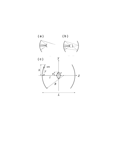
Figure 1: (a) An unstable cavity is built of a spherical concave mirror (with radius $R$) and a cylindrical convex one (with radius $r$) at distance $l<R-r$. (b) Two unstable cavities are coupled to form a single cavity which is globally stable for $L<2R$. (c) Schematic diagram of the cavity model utilized in the numerical analysis. For all calculations in this Letter we have assumed $a=0.003$ and $b=0.025$ where all length are expressed in meters not . On the left mirror the position $y$ and the velocity $\mathbf{v}$ define the geometry of the chaotic scattering.

The basic idea is as follows (Fig. 1a). An unstable optical cavity Siegman (1996) can be built with a concave (focussing) mirror with radius of curvature $R$ and a convex (dispersing) mirror with radius of curvature $r$ at distance $l<R-r$. This unstable cavity has exponential sensitivity to initial conditions Ott (2002) but does not have mixing properties because an escaping ray never comes back; therefore chaos cannot occur. We overcome this difficulty in the way illustrated in Fig. 1b: a second cavity, mirror-symmetric to the first, is utilized to recollect rays leaving the first cavity and eventually put them back near the starting point. The final design of our composite cavity is depicted in Fig. 1c; $L$ is the total length of the cavity and satisfies the relation $L<2R$ in order to assure the geometrical stability of the whole system. Depending on the values of $R$, $r$ and $l$ each of the two sub-cavities can be either stable or unstable. For $l<R-r$ they are unstable: this case is the first object of our study (see below for the case $R-r<l<R$ where the two sub-cavities are stable). A generic ray lying in the plane of Fig. 1c and undergoing specular reflections on the cavity mirrors, will never leave this plane. As will be shown in this Letter, the 2D ray dynamics in this plane can be completely chaotic; consequently, from now on, we restrict our attention to the truly 2D cavity shown in Fig. 1c.

The study of the chaotic properties of our composite cavity, starts from the analogy between geometric optics of a light ray and Hamiltonian mechanics of a point particle Arnold (1978). In this spirit we consider the light ray as a unit-mass point particle that undergoes elastic collisions on hard walls coincident with the surfaces of the mirrors. Between two consecutive collisions, the motion of the point particle is determined by the free Hamiltonian $H=\mathbf{p}^{2}/2$ whereas at a collision the position $\mathbf{r}(t)$ and the velocity $\mathbf{v}(t)$ ($|\mathbf{v}(t)|=1\;m/s$ throughout this Letter) of the particle satisfy the law of reflection:

$$\mathbf{r}(t_{+})=\mathbf{r}(t_{-}),\qquad\mathbf{v}(t_{+})=(\mathbf{1}-2\mathbf{n}\mathbf{n})\mathbf{v}(t_{-}),$$ (1)

where $t_{\pm}=t\pm 0^{+}$, $\mathbf{n}$ is the unit vector orthogonal to the surface of the mirror at the point of impact and the second rank tensor $\mathbf{n}\mathbf{n}$ has Cartesian components $[\mathbf{n}\mathbf{n}]_{ij}=n_{i}n_{j}$ $(i,j=1,2)$. The dynamics described by Eqs.(1) preserves both the phase space volumes and the symplectic property Ott (2002). The losses of a cavity due to finite reflectivity of the mirrors can be quantified by the finesse of the cavity, that is the number of bounces that leads to $e^{-1}$ energy decay. For optical cavities realized with commercially available mirrors values for the finesse of $10^{5}$ (or even larger) can be achieved not . In our model we assume a mirror reflectivity equal to $100\%$ for all mirrors and consequently we restrict ourselves to losses due to the finite transverse dimensions of the concave mirrors (parameter $b$ in Fig. 1c). If chaos occurs, almost all trajectories will escape in the end Ott (2002); the key question is whether a typical trajectory will survive sufficiently long that chaos is still a useful concept.

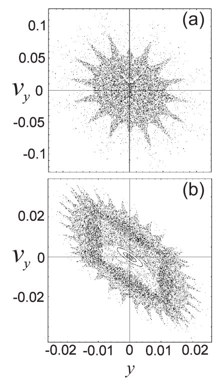
Figure 2: Poincaré maps obtained as described in the text. In both cases the cavity parameters $a$ and $b$ are chosen as: $a=0.003$, $b=0.025$. Note that $v_{y}\simeq 0.1$ corresponds to an angle of incidence of about $6^{\circ}$ not . (a) Hard-chaos configuration: $R=1$, $r=0.25$, $l=0.04$. A single chaotic orbit is shown. (b) Soft-chaos configuration: $R=1$, $r=0.9$, $l=0.45$. Three stable orbits (concentric ellipses) and a single chaotic one are shown.

We use the Poincaré surface of section (SOS) Ott (2002) as a tool to display the dynamical properties of our composite cavity. There are several possibilities for defining a SOS; we choose as reference surface the left mirror, plotting $y$ and $v_{y}$ each time the ray is reflected by that mirror. In Fig. 2a we show the SOS generated by a single orbit for a cavity configuration such that $l<R-r$ (geometrically unstable sub-cavities). Apparently, hard chaos occurs; the unstable periodic orbit bouncing along the $Z-$axis of the cavity is represented by an hyperbolic fixed point on the SOS. The explicit value of the Lyapunov exponent for this orbit can be easily calculated exploiting the above mentioned analogy between geometric optics and Hamiltonian mechanics. We recall that the magnification $M$ Siegman (1996) of the cavity shown in Fig. 1a can be easily calculated in terms of $m$, the half of trace of the $ABCD$ matrix of the cavity:

$$M=m+(m^{2}-1)^{1/2},$$ (2)

where

$$m=2\left(1-\frac{l}{R}\right)\left(1+\frac{l}{r}\right)-1.$$ (3)

Since the $ABCD$ matrix of the cavity coincides with the monodromy matrix H. -J. Stöckmann (1999) for the unstable periodic orbit bouncing back and forth along the $Z$-axis, the positive Lyapunov exponent $\lambda_{0}$ for such orbit is given by:

$$\lambda_{0}=\frac{v}{2l}\ln M,\qquad(v=1m/s).$$ (4)

With the numerical values utilized for Fig. 2a we obtain $M\simeq 1.94$ and $\lambda_{0}\simeq 8.27$ (in units of $s^{-1}$).

We may now ask what will happen if the two sub-cavities of Fig. 1c are stable (i.e. $R-r<l<R$) so that there is no magnification. Will the chaoticity (partly) survive, or not? As shown in Fig. 2b we find that in that case the periodic orbit bouncing along the $Z-$axis is represented by an elliptical fixed point on the SOS, surrounded by a KAM island of stability in which three stable trajectories are clearly visible. Surprisingly, we find that despite the stability of the two sub-cavities, the KAM island of stability is embedded in a sea of chaotic trajectories with a positive Lyapunov exponent. Therefore depending on the values of the parameters $R$, $r$ and $l$ our cavity can exhibit either fully chaotic behavior, or soft-chaotic behavior with coexistence of ordered and stochastic trajectories.

Table 1: Results for Lyapunov exponents $\lambda_{1}$ for different cavity configurations which are specified by $l_{R}$ ($l_{L}$) as the length of the right (left) sub-cavity and $R$ ($r$) as the radius of curvature of the concave (convex) mirror. All lengths are given in m, further details are given in the text.

Configuration	$R$	$r$	$l_{L}$	$l_{R}$	$\lambda_{1}$
$UU$	1	.25	.04	.04	$0.104\pm 0.004$
$US$	1	.90	.05	.30	$0.0165\pm 0.0002$
$SS$	1	.90	.45	.45	$0.0040\pm 0.0001$
$MM$	1	.80	.20	.20	$0.0090\pm 0.00015$
$SM$	1	.80	.40	.20	$0.0096\pm 0.0001$
$UM$	1	.80	.01	.20	$0.0191\pm 0.0004$

A rigorous theory for the calculation of average Lyapunov exponents, entropies and escape time for open systems, has been developed by Gaspard and coworkers in the last decade Gaspard (1998). In short, in chaotic open systems there exists a fractal set of never-escaping orbits, the so-called repeller Kadanoff and Tang (1984) on which quantities as the average Lyapunov exponents can be evaluated. In a Hamiltonian system with two degrees of freedom the Lyapunov exponents come in pairs $(\lambda_{i},\lambda_{-i})$, $(i=1,2)$ with $\lambda_{1}\geq\lambda_{2}=0$ and $\lambda_{i}+\lambda_{-i}=0$ Ott (2002). We have calculated Benettin and Strelcyn (1978); Dellago and Posch (1995) the values of $\lambda_{1}$ for different long-living trajectories belonging to the repeller for different cavity configurations; the “pairs rule” (sum of all Lyapunov exponents equal to 0) has been confirmed within our numerical accuracy. The results are shown in Table I. Each cavity configuration is labelled as $LR$ where $L,R=U,M,S$ are labels which indicate the stability properties of the left and right sub-cavity respectively: $U=$ Unstable ($m>1$), $M=$ Marginally stable ($m=1$), $S=$ Stable ($m<1$). In all cases we find a positive Lyapunov exponent which confirms that chaos has developed; the maximum value ($\lambda_{1}=0.104$) occurs for the $UU$ case. We stress the fact that the values for the parameters characterizing the different cavity configurations given in Table I are experimentally realistic (i.e. such mirrors are commercially available).

Note that the value $\lambda_{0}\simeq 8.27$ quoted above for the periodic orbit bouncing along the $Z-$axis of the unstable cavity is quite different from the average value $\lambda_{UU}\simeq 0.10$. We argue that this is due to the fact that the same unstable periodic orbit may be considered as an orbit of the single half-cavity (very open system: no chaos at all) or as an orbit of the overall composite cavity. Consequently the sub-cavity value for $\lambda_{1}$, even though it remains obviously the same, is “diluted” into the value for the whole cavity.

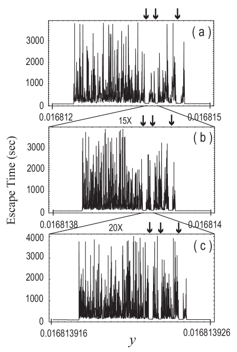
Figure 3: Escape-time as a function of the impact parameter $y$ for the same hard-chaos cavity configuration utilized in Fig. 2a, shown at different relative magnifications ($1\times$, $15\times$ and $20\times$) of the horizontal axis. The finite value ($\approx 4000$ secs) for each singular peak corresponds to the finite value ($6\times 10^{4}$) of the maximum number of bounces allowed in the simulations. In the three pictures are clearly visible the “windows of continuity” (arrows) and the repetition of the same pattern on different scales (self similarity).

It is possible to obtain a picture of the repeller set by plotting the escape-time function Ott (2002). For each trajectory starting at position $y$ (“impact parameter”) and horizontal velocity $\mathbf{v}$ on the left mirror (see Fig. 1c), we calculate the time at which the last bounce occurs before the ray leaves the cavity. Trajectories which escape in a finite time (almost all), give a finite value for the escape-time function, whereas trapped orbits are represented as singular points. By definition, all initial conditions leading to a singularity of the escape-time function belong to the repeller itself. In Fig. 3 we show a portion of the escape time function for a hard-chaos cavity configuration ($UU$: same parameters as in Fig. 2a). In Fig. 3a we observe clearly three “windows of continuity” Gaspard (1998) (arrows) for which the escape time function has a small value. Actually, Fig. 3a as a whole results from the blow-up of the escape time function in a region bounded by two other windows of continuity which are partially visible on the left and the right side of the figure. Consecutive blow-ups of Fig. 3a are shown in Fig. 3b and Fig. 3c. We note that going from one picture to the next both the density and the height of the singular peaks increase thus indicating that the repeller set is dense. Moreover the windows of continuity act as convenient markers of the self-similar nature of the pattern as a whole; this self-similarity strongly suggests that the escape time function is singular on a fractal set, as expected for a repeller. The dense occurrence of singular points is a clear signature of the mixing mechanism due to the confinement generated by the outer concave mirrors. Note that typical escape times are much larger than $1/\lambda_{UU}$, thus allowing ample time for chaos to develop.

Thus, we have shown that it is possible to build, with commercially available optical elements, a composite optical cavity which displays classical chaotic properties. Despite the “local” Hamiltonian structure of its phase space our optical cavity is, as we had anticipated, an open system. Opening up a closed chaotic Hamiltonian system may generate transiently chaotic behavior due to the escape of almost all the trajectories Schneider et al. (2002) and our composite cavity promises an easy experimental realization thereof. Evidence for ray chaos comes both from the computation of Lyapunov exponents and from the plot of the escape time functions. The huge density of singular points in the escape time functions is a strong indication that the anticipated mixing works: unstable orbits which leave one half-cavity are recollected by the other half-cavity until they become again unstable and come back to the first cavity. Orbits for which this process is repeated forever generate singularities in the escape function.

Finally, the most convenient experimental way to realize the composite cavity as a 3D system seems to be by using spherical elements for focussing mirrors and a cylindrical element for the dispersing one. A bi-convex cylindrical mirror (with $X$ as the axis of the cylinder) is dispersing for trajectories lying in a plane orthogonal to the $X$-axis and is neutral (flat surface) for trajectories in a plane containing the $X$-axis itself. In this case Fig. 1a represents the unstable cross section of the left sub-cavity. The realization of such an open chaotic cavity in the optical domain opens a broad perspective: many quantum-optics experiments can now be done on a practical chaotic system Beenakker et al. (2000); Misirpashaev and Beenakker (1998). Such experiments will greatly benefit from the ease of manipulation and control offered by the macroscopic nature of our composite cavity: work along these lines is in progress in our group.

This project is part of the program of FOM and is also supported by the EU under the IST-ATESIT contract. We acknowledge J. Dingjan and T. Klaassen for stimulating discussions.

References

- Haake (2000) F. Haake, Quantum Signatures of Chaos (Springer, Berlin, 2000), 2nd ed.
- H. -J. Stöckmann (1999) H. -J. Stöckmann, Quantum Chaos, An Introduction (Cambridge University Press, 1999), 1st ed.
- Dingjan et al. (2002) J. Dingjan, E. Altewischer, M. P. van Exter, and J. P. Woerdman, Phys. Rev. Lett. 88, 064101 (2002).
- P. Pechukas (1984) P. Pechukas, J. Phys. Chem. 88, 4823 (1984).
- H. Alt et al. (1997) H. Alt et al., Phys. Rev. E 55, 6674 (1997).
- Wilkinson et al. (2001) P. B. Wilkinson, T. M. Fromhold, R. P. Taylor, and A. P. Micolich, Phys. Rev. Lett. 86, 5466 (2001).
- C. Gmachl et al. (1998) C. Gmachl et al., Science 280, 1556 (1998).
- Beenakker et al. (2000) C. W. J. Beenakker, M. Patra, and P. W. Brouwer, Phys. Rev. A 61, 051801(R) (2000).
- Hackenbroich et al. (2001) G. Hackenbroich, C. Viviescas, B. Elattari, and F. Haake, Phys. Rev. Lett. 86, 5262 (2001).
- Misirpashaev and Beenakker (1998) T. S. Misirpashaev and C. W. J. Beenakker, Phys. Rev. A 57, 2041 (1998).
- Jenkins and White (1981) F. A. Jenkins and H. E. White, Fundamental of Optics (McGraw-Hill, 1981), 4th ed., pag 536.
- Fukushima et al. (1997) T. Fukushima, S. A. Biellak, Y. Sun, and A. E. Siegman, Opt. Express 2, 21 (1997).
- A. Aiello et al. (2003) A. Aiello et al. (2003), in preparation.
- (14) With values for , , , and as chosen in Figs. 1,2, the maximum angle of incidence on the mirrors occurring in Fig. 2 is ; this is sufficiently small as not to compromise the high reflectivity of a multilayer dielectric mirror.
- Siegman (1996) A. E. Siegman, Lasers (University Science Books, Mill Valley, CA, 1996).
- Ott (2002) E. Ott, Chaos in Dynamical Systems (Cambridge University Press, 2002), 2nd ed.
- Arnold (1978) V. I. Arnold, Mathematical Methods of Classical Mechanics (Springer, New York, 1978).
- Gaspard (1998) P. Gaspard, Chaos, Scattering and Statistical Mechanics (Cambridge University Press, 1998), 1st ed.
- Kadanoff and Tang (1984) L. P. Kadanoff and C. Tang, Proc. Natl. Acad. Sci. U.S.A. 81, 1276 (1984).
- Benettin and Strelcyn (1978) G. Benettin and J. M. Strelcyn, Phys. Rev. A 17, 773 (1978).
- Dellago and Posch (1995) C. Dellago and H. A. Posch, Phys. Rev. E 52, 2401 (1995).
- Schneider et al. (2002) J. Schneider, T. Tél, and Z. Neufeld, Phys. Rev. E 66, 066218 (2002).